Machine Learning Classification of Food
The MIT Faculty has made this article openly available.
Please share
how this access benefits you. Your story matters.
Citation
Schroeder, Vera et al. "Chemiresistive Sensor Array and Machine
Learning Classification of Food." ACS Sensors 4, 8 (July 2019): 2101–
2108 © 2019 American Chemical Society
As Published
http://dx.doi.org/10.1021/acssensors.9b00825
Publisher
American Chemical Society (ACS)
Version
Author's final manuscript
Citable link
https://hdl.handle.net/1721.1/128141
Terms of Use
Article is made available in accordance with the publisher's
policy and may be subject to US copyright law. Please refer to the
publisher's site for terms of use.
Chemiresistive Sensor Array and Machine Learning Classification of Food
Vera Schroeder,
a‡Ethan D. Evans,
b‡You-Chi Mason Wu,
aConstantin-Christian A. Voll,
aBenjamin R.
McDonald,
aSuchol Savagatrup,
aand Timothy M. Swager
a, *a
Department of Chemistry and Institute for Soldier Nanotechnologies, Massachusetts Institute of Technology, 77
Massachusetts Avenue, Cambridge Massachusetts 02139, United States
b
Department of Biological Engineering, Massachusetts Institute of Technology, Cambridge Massachusetts 02139, United
States
Keywords: chemical sensor, sensor array, carbon nanotubes, electronic nose, authentication, time series classification,
feature selection, nearest neighbors
Supporting Information Placeholder
ABSTRACT: Successful identification of complex odors by sensor arrays remains a challenging problem. Herein, we report robust, category-specific multiclass-time series classification using an array of 20 carbon nanotube-based chemical selectors. We differentiate between samples of cheese, liquor, and edible oil based on their odor. In a two-stage machine-learning approach we first obtain an optimal subset of sensors specific to each category and then validate this subset using an independent and expanded dataset. We determined the optimal selectors via independent selector classification accuracy as well as a combinatorial scan of all 4,845 possible four selector combinations. We performed sample classification using two models – a k-nearest neighbors model and a random forest model trained on extracted features. This protocol led to high classification accuracy in the independent test sets for five cheese and five liquor samples (accuracies of 91% and 78% respectively) and only a slightly lower (73%) accuracy on a five edible oil dataset.
The three major functions of the human olfaction system are related to social communication,1,2 avoidance of environmental
hazards,3 and ingestive behavior.4–6 Our ability to successfully
differentiate between stimuli in these applications is enabled by more than 1000 distinct olfactory receptors (ORs).7 Activation of
an OR by an odorant generates an electronic signal that is transmitted to the brain.8 Each OR recognizes several odorant
molecules and each odorant molecule is recognized by several distinct ORs. The identification of a specific odorant molecule, or mixture thereof, is confirmed by the activation of a specific combination of ORs.8,9 Thus, the olfaction system of humans and
animals can identify complex mixtures of chemicals and not just pure chemicals against an odorless background.
Array-based chemical sensors follow a similar biomimetic approach. Detection of chemical inputs is achieved through a combination of multiple sensing channels where each channel responds to several analytes.10,11 Single-walled carbon nanotube
(SWCNT) chemiresistors and carbon nanotube-based electrochemical sensors have been shown to provide suitable platforms for array-based detection of various gases.12 Several
sensor arrays comprising CNT-based sensing channels have been used to discriminate between single volatile organic compound (VOC) vapors,13–18 inorganic gases,19,20 and biological samples.21– 24 However, few reports have been published on the differentiation
between food samples, among them are the determination of caffeine content in coffee,25 the electrochemical detection and
differentiation between rice wines,26 electrochemical determination
of capsaicin content of hot sauces,27 and chemiresistive
differentiation of liquors using multi-walled CNT/polymer composites.28,29
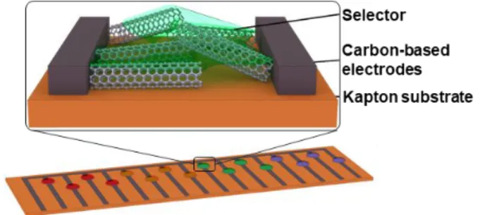
Herein, we differentiate between complex odors using an array of 20 SWCNT-based chemiresistive sensors (Figure 1). As a proof-of-principle system we investigated samples of different food item categories – cheese, liquor, and edible oil. The odor compounds of these food items include distinct combinations of a multitude of sulfur compounds, alcohols, ketones, aldehydes, esters, organic acids, alkanes, and aromatic compounds.30–40 We
strategically designed the sensor array to include selectors that can interact with odor compounds containing these functional groups. In addition to the choice of selectors, a similarly sophisticated analysis of the sensing data is necessary to enable successful differentiation.
Figure 1. Schematic of sensing device with carbon-based
electrodes deposited on a Kapton substrate. The active layer of SWCNTs and selectors is deposited between the electrodes. All 20 selectors are listed in Table S1.
Previously, classification in gas sensing applications has been performed by discriminant factor analysis (DFA) to diagnose disease,22 principle component analysis (PCA) to differentiate
between VOCs,13 a neural network model to differentiate between
formaldehyde and ammonia gas,19 and a support vector machine to
differentiate between NO2, NH3, EtOH, and acetone.41 These
methods generally only use a limited number of features from the sensing response (sometimes with additional metadata concerning the specifics of the sensing apparatus). In contrast, we use the entire time series of the sensor response or a large set of diverse features extracted from the exposure-recovery cycle to perform accurate classification.
Traditional time series classification has relied on nearest neighbor approaches via either Euclidean or dynamic time warping-based (a means of aligning time series) distance comparisons used to calculate a similarity between two time series.42–44 Similarly, time series decompositions where the data is
represented as piecewise linear45 or piecewise polynomial
segments46 as well as feature extraction techniques, combined with
more traditional machine learning models like random forests (RF) or support vector machines47 have also been proposed. Lately,
ensembles of models have become a popular choice for high
ACS Paragon Plus Environment
1
2
3
4
5
6
7
8
9
10
11
12
13
14
15
16
17
18
19
20
21
22
23
24
25
26
27
28
29
30
31
32
33
34
35
36
37
38
39
40
41
42
43
44
45
46
47
48
49
50
51
52
53
54
55
56
57
58
59
performance time series classification leveraging potentially multiple techniques with different models.48 Often, improvement
over the simple k-nearest neighbors algorithm (KNN) is difficult, questioning the need for these highly sophisticated methods49 that
often require larger training datasets. In this study, we found a RF model trained on features extracted from the sensing data (featurized-RF model, f-RF) to be a highly accurate method for analyzing time series data of very similar food samples. This model can classify samples of cheese, liquor, and edible oil with up to 91% accuracy.
EXPERIMENTAL SECTION
Sensor array. The sensing substrates are made of carbon-based
electrodes (1 mm gap width) on a Kapton support. One substrate contains 16 individual working electrodes with a shared counter electrode separated by a gap of 1 mm. The active material of the sensor channels consists of SWCNTs as a transduction material and a chemical selector (S1-S20) as a selective moiety. The active material is deposited between the electrodes in a one- or two-step process. For the one-step process, 1 µl of a dispersion of selectors S17, S18, or S19 and SWCNTs in ortho-dichlorobenzene (o-DCB) was drop-casted between the electrodes and dried in vacuo. For the two-step process, 1 µl of a dispersion of SWCNT in o-DCB was drop-casted between the electrodes and dried in vacuo, then 1 µl of a solution of the selector S1, S2, S3, S4, S5, S6, S7, S8, S9, S10, S11, S12, S13, S14, S15, S16, or S20 was drop-casted on top of the SWCNT layer and again dried in vacuo. Chemical structures of the selectors and detailed experimental procedures can be found in the supporting information and all solvents, concentrations, and dispersion parameters are listed in Table S1.
Gas sensing data. During the gas sensing experiment, 0.100 V
was applied across the sensing electrodes and the resulting current was measured as a function of time. All gas sensing data was collected using air (approximately 40 % relative humidity) as the carrier gas at a flow rate of 100 ml/min. The sample gas was generated by heating the food sample to 30-50 °C and collecting the headspace over the sample at a distance of 3 cm. During the gas measurement, the active material was exposed to the sample gas for 120 s followed by a 600-900 s recovery period under air flow.
Machine learning model training. We used 300 s of sensing
data (120 s of exposure, and 180 s of recovery) to train either a KNN model (k=1) that directly used the time series data or a f-RF (100 estimators) using features extracted via tsfresh. Tsfresh extracts 794 features ranging from the coefficients of a continuous wavelet transform or fast Fourier transform to parameters like time series length, mean, max, and median among many others.50 Data
from each selector were used to train individual models for classification using Scikit-learn.51 The 20 selector-three-class
models were trained with a stringent 0.67:0.33 train:test split while the four selector-five-class models were trained with a 0.80:0.20 train:test split. The combinatorial selector scan was performed on all 4,845 possible combinations of 4 out of 20 selectors. Final model accuracy was assessed via a 50× repeated model training on randomly shuffled train:test splits. Complete protocols for the computational analysis and model building can be found in the supporting information.
RESULTS AND DISCUSSION
Collection of sensing data. To develop a sensing system that
can differentiate between complex organic odor mixtures, the choice of selectors is critical. We assembled an array of 20 selectors including: transition metal complexes (S1, S2, S3, S4) to bind organic acids52 and sulfur-containing compounds, ionic
liquids (S5, S6, S7, S8) to interact with ketones, aldehydes,
alkanes, and aromatic compounds;53 porous polymers (S9, S10,
S11, S12) to sequester a large number of organic vapors;54,55
cavitand molecules (S13, S14, S15, S16, S20) for detection of aromatic compounds and alcohols with size exclusion properties;15,17 and metalloporphyrins (S17, S18) to bind amines,
alcohols, ketones, alkanes, and aromatic compounds.13,56
The input data for our machine learning algorithms consist of the chemiresistive responses of the active material to the sample odor. We examined five categories of samples, including cheeses (cheddar, cream cheese, Cambozola, Mahón, and pecorino), liquors (gin, tequila, rum, vodka, and whiskey), and edible oils (canola, olive, coconut, toasted sesame, and walnut oil). During the gas measurement, the active material – SWCNT and selector – was exposed to the sample odor for 120 s followed by a 600-900 s recovery period under air flow. The response is recorded as the conductance through the active material at a constant applied voltage (0.100 V).
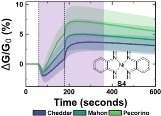
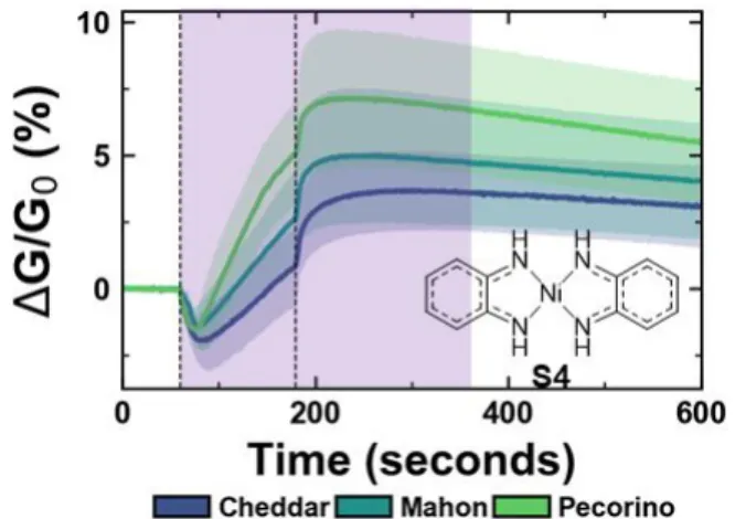
Figure 2 shows the representative response of average change in conductance normalized to the conductance at the start of the exposure (ΔG/G0) for one selector (S4) towards the odor of three
different cheeses: cheddar, Mahón, and pecorino. The data used for classification consists of all time points in the 300 s time period after the start of the exposure (120 s of exposure, and 180 s of recovery, purple shaded area in
Figure 2).
1
2
3
4
5
6
7
8
9
10
11
12
13
14
15
16
17
18
19
20
21
22
23
24
25
26
27
28
29
30
31
32
33
34
35
36
37
38
39
40
41
42
43
44
45
46
47
48
49
50
51
52
53
54
55
56
57
Figure 2. Example of sensing response for one selector (S4)
towards cheddar, Mahón, and pecorino. The response is represented as a change in conductance normalized to the conductance at the start of the exposure (ΔG/G0). The exposure
starts at t = 60 s and ends at t = 180 s (marked by dashed vertical lines). The response is an average of 12 separate sensing experiments, the blue/green shaded areas represent the standard deviation of the response. The purple shaded area represents the data used for classification.
Selector analysis on three-class datasets. When designing a
sensor array, including sensor channels that have insignificant signal or the same signal for all samples weakens the overall performance of the array. To ensure we only use selectors that have high prediction ability, we identified which of the 20 selectors demonstrates the highest accuracy in differentiating between the food samples. For this, we collected 12 sets of sensing data for each one of the 20 selectors and for three items from each category (2,160 individual sensing traces). To evaluate the classification utility of the selectors in our sensor array, we built two models. The first model was the f-RF model trained on a set of features extracted using the tsfresh computational package50 from each selector time
series. The second model directly leverages the time-dependent nature of the data via a KNN model for which a Euclidean distance metric was used to measure time series similarity. Importantly and in contrast to typical analyses, both models rely on data from both the initial exposure and recovery time period, as the curvature and
absolute values for both of these periods provides valuable time-based patterns. The models are used to differentiate between three food items from each category: for cheese, the classes include cheddar, Mahón, pecorino; for liquor, the classes include rum, vodka, whiskey; for edible oil the classes include canola, olive, walnut.
Each of the 20 selectors was analyzed independently using both models on held-out test sets; 67% of the collected data sets were used for training the model (training set) and the remaining 33% were used to test the model (test set). The models assign the samples of the test set into classes – like cheddar, Mahón, pecorino for the cheese samples.
The accuracy for each selector was then calculated as the fraction of correct assignment made by the f-RF or KNN model corresponding to that selector:
𝐴𝑐𝑐𝑢𝑟𝑎𝑐𝑦 =𝑛𝑢𝑚𝑏𝑒𝑟 𝑜𝑓 𝑐𝑜𝑟𝑟𝑒𝑐𝑡 assignments 𝑛𝑢𝑚𝑏𝑒𝑟 𝑜𝑓 𝑡𝑜𝑡𝑎𝑙 assignment
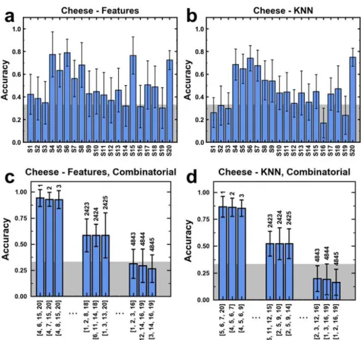
Figure 3a,b show the accuracies for f-RF and KNN models when differentiating between three cheese samples (Figure S13 shows analogous graphs for liquor and edible oils). Selectors that performed well in an f-RF model often showed high accuracies in the KNN model, suggesting the importance of specific selectors for each use case. Similarly, selectors showing near random performance in one model, often display commensurate classification ability in the other model. S4 for example, demonstrates reasonable test set accuracy for classification of the three cheeses using the f-RF (0.78±0.20) and the KNN (0.69±0.14) model. Across data sets (cheese vs. liquor for instance), different selectors exhibit high performance; selectors working well in one use-case may have lower classification ability in another (Figure S13). This observation can be ascribed to the difference in chemical makeup of the items in these categories. One of the selectors showing high accuracy in the cheese use-case is S4, a nickel bis(ortho diiminosemiquinate) known to detect organic acids.52 S5
and S6 are two methylimidazolium based ionic liquids, 1-(2-(2-(2-hydroxyethoxy)ethoxy)ethyl)-3-methylimidazolium chloride and 1-(nonyl)-3-methylimidazolium hexafluorophosphate, designed to interact with aldehydes and ketones.53 Organic acids, aldehydes
and ketones are all important aroma compounds with moderate volatility which can be found in the odor of cheese.31,57,58
ACS Paragon Plus Environment
1
2
3
4
5
6
7
8
9
10
11
12
13
14
15
16
17
18
19
20
21
22
23
24
25
26
27
28
29
30
31
32
33
34
35
36
37
38
39
40
41
42
43
44
45
46
47
48
49
50
51
52
53
54
55
56
57
58
59
Figure 3. a,b) Selector accuracies for both the (a) f-RF and (b) KNN models using single selectors for differentiating between cheddar,
Mahón and pecorino cheese. The shaded, grey area corresponds to random guessing (33 % accuracy between cheddar, Mahón, and pecorino), selectors with accuracies around this threshold do not assist in this particular application. c,d) Example results from the combinatorial selector scan for both the (a) f-RF and (b) KNN models on the cheese dataset (cheddar, Mahón and pecorino) using combinations of four selectors. Plotted are the top three (1-3), three medium (2423-2425), and the bottom three (4843-4845) combinations. Each selector combination was trained 27 times, plotted are the average accuracies and standard deviations.
Combinatorial selector scan. While using each selector
individually led to moderate success in classification, we suspected that using combinations of multiple selectors will enable classification with higher fidelity. To exhaustively determine an optimal set of selectors for model building, analysis, and collection of additional data sets we trained and tested f-RF and KNN models on all possible combinations of 4 selectors (4,845 combinations).
The combinatorial analysis revealed many selector combinations with similar scores, nonetheless common trends emerged internal to a dataset category (Figure 3c,d Figure S15). These trends often mapped to the results from the individual selector analysis. Across item categories, different selector combinations showed varying levels of usefulness for each individual classification problem (Figure S15), highlighting the need for tuning the selector panel when confronted with a new category of interest.
Focusing only on the highest accuracy selector combination in all three item categories, the f-RF models typically outperformed the simpler KNN models (Figure 4). We propose that this results from the extraction of more descriptive temporal features not accounted for in an isolated time point-to-time point distance calculation used in the KNN model in combination with a more expressive random forest model. Indeed, principal component analysis (PCA) on the features extracted from the three-item datasets often showed a degree of class separability using only the first three principle components (Figure S16).
Based on the information from the combinatorial selector analysis (Figure 3c,d) along with that of the individual selector
analysis (Figure 3a,b), we picked four selectors for follow up analysis and validation for each sample category. For the cheese use-case, we identified S4, S5, S6, and S20 as a high-performing selector combination. We performed the analogous combinatorial analysis for the other two use-cases – liquor and edible oil – to identify use-case specific high-performing sector combinations (Figure S13, Figure S15). The selector combinations for liquor (S7, S8, S12, and S15) and the selector combination for edible oil (S5, S7, S8, and S13) both consist of three methylimidazolium-based ionic liquids and one calix[4]arene. The combinatorial approach leads to higher classification accuracy across all use-cases and both models. For example, the maximum test set accuracy for a single selector when differentiating between cheddar, Mahón and pecorino cheese is 0.79±0.12 (S6) whereas the combinatorial approach reaches 0.94±0.08 (f-RF). Going forward, all analysis was performed using the combinatorial approach.
1
2
3
4
5
6
7
8
9
10
11
12
13
14
15
16
17
18
19
20
21
22
23
24
25
26
27
28
29
30
31
32
33
34
35
36
37
38
39
40
41
42
43
44
45
46
47
48
49
50
51
52
53
54
55
56
57
Figure 4. Selector scan results showing only the highest accuracy
selector combinations for each use case.
Optimal selector combination performance on independent five-class datasets. With our optimized combination of selectors
in hand, we significantly increased the difficulty of classification problem by expanding the number of items in each category from three to five. Notably, there is the question of whether selectors chosen for classification can have utility for not only to the pre-screened class, but also to additional examples (classes) from the same general type of samples. For cheese, the expanded selection includes cheddar cheese, Mahón, Cambozola, cream cheese, and pecorino; for liquor, the expanded selection includes rum, vodka, whiskey, gin, and tequila; for edible oil the expanded selection includes canola, olive, walnut, coconut, and toasted sesame oil. For this validation of our methodology, we collected new sets of data for all samples and retrained all models.
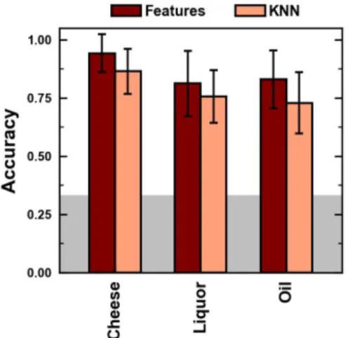
Even for these expanded item categories, the newly trained models show high levels of classification accuracy (Table 1). Between the three item categories, cheese was the easiest to classify
with a test set accuracy of 0.91 followed by liquor at 0.78 and oil being the most challenging with a reasonable accuracy of 0.73 when using the f-RF model. The simpler KNN model displayed a reduced performance across the board with an accuracy of 0.73 for the cheese data set while much lower values near 0.40 were observed for the liquor and oil data. These values are still significantly higher than that of random guessing (0.2) for a five-class problem. This again highlights the additional important information contained in the time series that a simple point-to-point distance measurement does not capture. Further, these results speak to the chemical compositions of the odor of the different samples, suggesting the volatiles in oil to be more similar between samples than those of cheese, making the classification problem more challenging.
Table 1: Optimal 4-selector test set accuracya analysis on the
five-class classification problems for both the f-RF and KNN models. Cheese (4,5,6,20) Liquor (7,8,12,15) Oil (4,7,9,13) f-RF 0.91 ± 0.05b 0.78 ± 0.08 0.73 ± 0.07 KNN 0.73 ± 0.06 0.40 ± 0.09 0.36 ± 0.08
aAverage accuracies are calculated via 50 f-RF or KNN models
trained and tested on shuffled data splits. bError values are standard
deviations.
Analyzing the average time course values for each sample and selector often revealed only subtle differences between the different classes with several notable cases. Typically, the overall shape of the selector response curve was similar between samples of a category (with differences in the response amplitude). For example, in the five-cheese data, the Cambozola cheese displayed similar temporal dynamics, but with a much higher selector response (Figure 5, purple line).
ACS Paragon Plus Environment
1
2
3
4
5
6
7
8
9
10
11
12
13
14
15
16
17
18
19
20
21
22
23
24
25
26
27
28
29
30
31
32
33
34
35
36
37
38
39
40
41
42
43
44
45
46
47
48
49
50
51
52
53
54
55
56
57
58
59
Figure 5. Sensing response for a) S4, b) S5, c) S6, and d) S20 towards five cheeses. The response is represented as a change in conductance
normalized to the conductance at the start of the exposure (ΔG/G0). Each exposure starts at t = 60 s and ends at t = 180 s (marked by dashed
vertical lines). Each response is an average of 40 separate sensing experiments, the shaded area represents the standard deviation of the response.
It should not be overlooked, however, that several visually distinct temporal traces were observed (S4,S20 in the cheese data Figure 5a,d; S7 in the liquor data, Figure S17a; S13 in the edible oil data Figure S18d). In line with the lower accuracy of the five-oil data, the time course analysis revealed that many of the five-oils had overlapping temporal behavior in both the exposure and recovery periods with only subtle differences in the curvature. It is this subtle difference that the featurization protocol most likely leverages to gain a reasonable (0.73) accuracy but something the KNN Euclidean distance cannot overcome (0.36), leading to its significantly lower performance.
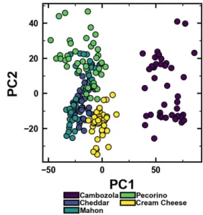
Extracted feature analysis. We took two approaches to better
understand the extracted features, the first is a dimension reduction (PCA), while the second is a feature-by-feature importance analysis. PCA analysis of extracted features of the five-class datasets again revealed decreased class separability going from cheese to liquor and finally to oil (Figure 6, Figure S19, S20, S21). As expected from the time course analysis, Cambozola cheese showed complete separation (along PC1). Nonetheless, after reduction of the sensing data to just a handful of principle components we observe significant overlap between the majority of the cheese classes (Figure 6). More class overlap was observed for the liquor samples with gin and whiskey displaying the most separability from the other examples (Figure S20). Finally, in the edible oil data, nearly all classes showed significant overlap along
the first two principle components, again corroborating the reduced model performance.
Figure 6. PCA analysis of extracted features from the five-cheese
dataset showing the first two principle components.
1
2
3
4
5
6
7
8
9
10
11
12
13
14
15
16
17
18
19
20
21
22
23
24
25
26
27
28
29
30
31
32
33
34
35
36
37
38
39
40
41
42
43
44
45
46
47
48
49
50
51
52
53
54
55
56
57
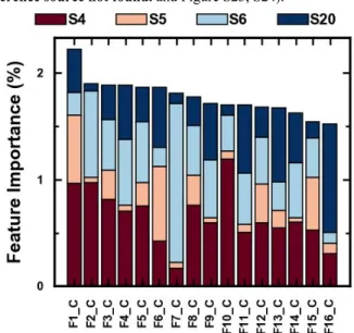
To better understand the f-RF models, we identified the features with the highest contribution to the prediction process. Figure 7 shows the 16 overall most important features – out of 794 total features – used in the f-RF model for the classification of five different cheeses. As expected from our findings of the PCA analysis, no single feature can be used solely for classification with many features showing less than 1% feature importance. This observation holds true for all three categories (Figure 7Error!
Reference source not found. and Figure S23, S24).
Figure 7. Top 16 overall most important features in the five-cheese
f-RF model. The importance is averaged over 50 f-RF models trained and tested on shuffled data splits. The top 16 features for cheese, liquor and edible oil are listed in Table S2-4.
The feature importance analysis also demonstrates that simple, descriptive features like maximum and minimum values, average values, and area under curve are not sufficient to perform this discriminative task (Table S2). In fact, the majority of the features used are coefficients from either a continuous wavelet transform (cwt features) or a fast Fourier transform (fFt features).
CONCLUSION
In this work, we demonstrated the classification of several complex odors using a chemiresistive sensing array in combination with a two-step machine learning approach. In doing so, we propose a general method for object classification that may be applied to a host of other challenging problems. With this method, we were able to differentiate between food samples with up to 91% accuracy. We envision this work to guide future research in two ways (1) our selector panel can be used to tackle a number of other challenging gas sensing problems like disease diagnostics, hazard detection, and food authentication, or (2) this general approach can also be used to quickly identify selectors from of a large panel of potential molecules.
ASSOCIATED CONTENT
Supporting InformationThe Supporting Information is available free of charge on the ACS Publications website. Included are descriptions of all chemical selectors used, additional details on sensor preparation, data collections and processing. Computational models and data handling are described as well as additional figures including optimal selector time series, PCA and feature importance analysis plots.
AUTHOR INFORMATION
Corresponding AuthorAuthor Contributions
‡These authors contributed equally.
Notes
The authors declare no competing financial interests.
ACKNOWLEDGMENT
This work was supported by the KAUST sensor project CRF-2015-SENSORS-2719 and the Army Research Office through the Institute for Soldier Nanotechnologies and the National Science Foundation (DMR-1410718). S.S. was supported by an F32 Ruth L. Kirschstein National Research Service Award. We want to thank Nathan A. Romero and Monika Stolar for their useful suggestions and fruitful conversations.