Coherent multi-exciton dynamics in semiconductor
nanostructures via two-dimensional Fourier
Transform optical spectroscopy
by
Katherine Walowicz Stone
B.S. Chemistry and B.S. Chemical Engineering
Michigan State University 2003
Submitted to the Department of Chemistry
in partial fulfillment of the requirements for the degree of
DOCTOR OF PHILOSOPHY
at the
MASSACHUSETTS INSTITUTE OF TECHNOLOGY
June 2009
c
° Massachusetts Institute of Technology 2009. All rights reserved.
Author . . . .
Department of Chemistry
May 6th, 2009
Certified by . . . .
Keith Adam Nelson
Professor of Chemistry
Thesis Supervisor
Accepted by . . . .
Robert W. Field
Chairman, Departmental Committee on Graduate Students
This doctoral thesis has been examined by a committee of the Department of Chemistry as follows:
Professor Jeffrey I. Steinfeld . . . . Chairperson
Professor Keith A. Nelson . . . . Thesis Supervisor
Coherent multi-exciton dynamics in semiconductor
nanostructures via two-dimensional Fourier Transform
optical spectroscopy
by
Katherine Walowicz Stone
B.S. Chemistry and B.S. Chemical Engineering
Michigan State University 2003
Submitted to the Department of Chemistry on May 6th, 2009, in partial fulfillment of the
requirements for the degree of DOCTOR OF PHILOSOPHY
Abstract
The Coulomb correlations between photoexcited charged particles in materials such as photosynthetic complexes, conjugated polymer systems, J-aggregates, and bulk or nanostructured semiconductors produce a hierarchy of collective electronic exci-tations (i.e. excitons, biexcitons, etc.) which may be harnessed for applications in quantum optics, light-harvesting, or quantum information technologies. These exci-tations represent correlations among successively greater numbers of electrons and holes, and their associated multiple-quantum coherences could reveal detailed in-formation about complex many-body interactions and dynamics. However, unlike single-quantum coherences involving excitons, multiple-quantum coherences do not radiate and they have largely eluded direct observation and characterization.
In this work, I present a novel optical technique, two-quantum two-dimensional Fourier transform optical spectroscopy, which allows direct observation of the dy-namics of multiple-exciton states that reflect the correlations of their constituent electrons and holes. The approach is based on closely analogous methods in nu-clear magnetic resonance, in which multiple phase-coherent fields are used to drive successive transitions such that multiple-quantum coherences can be accessed and probed. A spatiotemporal femtosecond pulse shaping technique has been used to overcome the challenge of control over multiple, noncollinear phase-coherent optical fields in the experimental geometries that are used to isolate selected signal contri-butions through wavevector matching. Results from a GaAs quantum well system reveal distinct coherences of biexcitons that are formed from two identical excitons or from two excitons whose holes are in different spin sublevels (“heavy-hole” and “light-hole” excitons). The biexciton binding energies and dephasing dynamics are
determined, and changes in the dephasing rates as a function of the excitation density are observed, revealing still higher-order correlations due to exciton-biexciton interac-tions. Two-quantum coherences due to four-particle correlations that do not involve bound biexciton states but that influence the exciton properties are also observed and characterized. I also present one-quantum two-dimensional Fourier transform optical spectroscopy measurements which show that the higher-order correlations isolated by two-quantum techniques are highly convolved with two-particle correlations in the conventional one-quantum measurements.
Thesis Supervisor: Keith Adam Nelson Title: Professor of Chemistry
Biographical Note
Katherine Walowicz Stone (a.k.a. Kathy or Kasia) was born Katherine Ann Walowicz on January 14th, 1980 in Detroit, MI to Leszek Jan and Karolina Walowicz. She has one younger sister, Annette Barbara (a.k.a. Basia). She was raised in Sterling Heights, MI. She attended Adlai E. Stevenson High School in her hometown where she was captain of the girls’ swim team and president of the National Honors Society. She also participated in Science Olympiad and Quiz Bowl. In 1998 she graduated Valedictorian of her class.
Kathy attended Michigan State University in East Lansing, MI from 1998 to 2003 and was a student in the Lyman Briggs School of Natural Science, the College of Engi-neering and the Honors College. In her freshman year she was a member of the Junior Varsity Womens’ Crew Team. In 1999, Kathy began doing undergraduate research with Professor Marcos Dantus in the Chemistry Department where her research focus included ultrafast laser pulse shaping and coherent control of multiphoton absorption in condensed phase systems. Kathy was also President of the Michigan Alpha chap-ter of Tau Beta Pi, an honors society for students in engineering, from 2001 to 2002. Kathy graduated from university in May, 2003 with a B.S. in Chemistry and a B.S. in Chemical Engineering and she received the Distinguished Award in Chemistry, which is awarded to the graduating student with the highest grade point average in chemistry courses.
Kathy married her high school sweetheart, Nicholas Charles Stone, in June of 2003 with whom she moved to Boston, MA shortly after to begin a Ph.D. program in physical chemistry in the Department of Chemistry at MIT. With Professor Keith Adam Nelson, she studied techniques for spatiotemporal shaping of ultrafast laser pulses for nonlinear spectroscopy applications. When Kathy is not in the laboratory, she enjoys video games, cooking, gardening and brewing beer.
Acknowledgments
I was about 14 years old when I first settled on pursuing science and engineering as a career. I can recall that my first opportunity to seriously attempt a scientific experiment was for my 9th grade biology class. Back then I was mainly interested in botany, so I devised an experiment to test the effect of different lighting conditions on plant growth. I planted identical catnip seeds in identical containers filled with identical soil types and placed one container on a window sill so that it could receive natural light, and the other I placed in the basement underneath a fluorescent lamp. The basement seeds sprouted within a week and the resulting plant grew long and spindly with short, narrow leaves. The window seeds took much longer to sprout and the matured plant was bushy with broad leaves. I was excited that I had gotten such dramatically different-looking plants and so I started to hypothesize all sorts of exotic explanations as to why I had obtained those results. However, when I presented my experiment to the class, my teacher ignored my wild conjectures and asked me to simply recount my basic experimental procedure. By the end, I had come to the simple conclusion that the basement plant was most likely not catnip (which, if you’ve ever seen a catnip plant, it’s not at all spindly and the leaves are broad with scalloped edges), but instead just a random weed that had sprouted because I just took the soil in which to plant the seeds from my backyard! In short, my first scientific experiment was a technical failure, but it did teach me a few simple aspects of the scientific method and I guess I have been honing those skills ever since. My professional development and accomplishments would not have been possible without the help of many people to whom I will attempt here to express my gratitude.
First, I would like to thank my Ph.D. research advisor, Keith Nelson. Keith has been an incredibly supportive mentor and guide. I have learned much about science from him and from the members of his team which he assembled. Keith taught me about the unique advantages afforded by pulse shaping which address the challenges of optical wave-mixing spectroscopy in very elegant ways, and I want to thank him for letting me pursue the techniques and experiments presented within these pages. I also want to thank him for believing in my work and supporting my efforts to publish the results and apply for a patent. Keith is also an extremely kind, friendly and fair person who is fun to be around.
I also want to thank several people who helped me directly with the work presented in this thesis. Daniel “Duffy” Turner is currently a 4th year graduate student in the Nelson group who joined the 2D FTOPT project in 2006. His assistance with main-taining the laser system and lab equipment, and making the actual measurements has been invaluable, and the modifications he made to optical setup made the rubidium measurements feasible. Kenan Gundogdu, who did a post-doc in the Nelson group from 2006 to 2008 and is now an Assistant Professor of Physics at North Carolina State University, helped me learn about 2D FT spectroscopy techniques and interpret the semiconductor quantum well measurements. Both Duffy and Kenan have been excellent co-workers with whom I’ve enjoyed many interesting and spirited scientific and non-scientific conversations. I also want to thank my collaborators at NIST/UC
Boulder, Steve Cundiff and the students and post-docs in his group, for the quantum well samples and their expertise in many-body phenomena in semiconductors.
I also want to thank the graduate student, Joshua Vaughan, and post-doc, Thomas Hornung, in the Nelson group who were my primary day-to-day mentors when I was a young graduate student. It was Josh who pioneered spatiotemporal pulse shaping in the Nelson group, and, along with Thomas, its application to nonlinear spectroscopy. They took me under their wing and taught me the basic optical techniques which are the foundation of my studies.
I also want to thank all the members of the Nelson group for creating a friendly and helpful working environment. Ka-Lo Yeh joined the group the same year as I. We started working on the same project, which diverged in the end, but she has remained a close collaborator and friend. I’ll always remember the time we travelled down from Seattle to San Francisco by car after the Ultrafast Phenomena conference in 2006 and visited Crater Lake, Portland, and the giant redwood forest. Darius Torchinsky was a graduate student in physics (although I won’t hold that against him) who is very knowledgable about spectroscopy in general, and was always good for a nice scientific (or not) discussion over coffee. I’d also like to thank Eric Statz and Ben Paxton for being a great resource for those laser, optic and cryostat-related technical issues. Dylan Arias and Patrick Wen are currently 2nd year graduate students embarking on exciting research projects related to 2D FTOPT and I’m looking forward to seeing their Ph.D. theses as well. I also wish to thank, for their advice and words of en-couragement, Prof. Bob Field, Prof. Jeff Cina, Prof. Thomas Feurer, Prof. Marcos Dantus, and Dr. Igor Pastirk.
I also wish to express my gratitude to members of my family. To my father, for supporting my choice to pursue a career in science and for always remaining enthusiastic about it. To my mother, for teaching me to stand up for myself. To my sister, who was my first friend. To my mother-in-law and father-in-law, Sally and Tom, for letting me be myself. To my brother-in-law, Adam, and his wife, Jenny, for sibling Thanksgiving and welcome respites from lab work. And to my other brother-in-law, Aaron, for forgiving me for stealing his older brother away and being like a younger brother to me too.
Last, but certainly not least, I want to thank my husband, Nick, for lovingly supporting me during my years in graduate school. I would not have had the courage to move away from home to begin this journey, or to continue it, without him, and so it is to Nick that I dedicate this work. Thank you for taking care of the house, the bills, the meals, the laundry, and for taking care of me. Thank you for being my best friend. Thank you for the trips to Maine, Cooperstown, and London. Thank you for bringing home our cat, Juliet. To me, you’ll never grow old, you’ll never die, and you’ll always eat oatmeal.
Contents
1 Introduction 21
2 Theory of 2D Fourier transform spectroscopy 27
2.1 Coupled two-particle correlations and one-quantum techniques . . . . 27
2.2 Four-particle correlations and two-quantum techniques . . . 32
3 Experimental methods 37 3.1 Introduction . . . 37
3.2 The Multidimensional Optical Spectrometer . . . 39
3.2.1 Diffractive beam shaping . . . 41
3.2.2 Diffraction-based spatiotemporal pulse shaping using a 2D SLM 43 3.3 2D FTOPT spectroscopy using SLM-delayed pulses . . . 46
3.3.1 Rotating frame detection . . . 46
3.3.2 Phase stability . . . 50
3.3.3 Pulse intensity roll-off correction . . . 51
3.3.4 Phase cycling . . . 54
3.3.5 Phasing the complex 2D FTOPT signal . . . 56
3.4 Conclusions . . . 57
4 Numerical models of exciton interactions 59 4.1 Introduction . . . 59
4.2 The optical Bloch equations . . . 60
4.3 The modified optical Bloch equations . . . 67
4.3.1 Local field effects . . . 70
4.3.2 Excitation-induced dephasing and frequency shift . . . 73
4.4 Conclusions . . . 77
5 Coupled and interacting excitons in semiconductors 79 5.1 Introduction . . . 79
5.2 2D FTOPT experiments on GaAs quantum wells . . . 87
5.2.1 One-quantum 2D FTOPT measurements . . . 93
5.2.2 Two-quantum 2D FTOPT measurements . . . 108
5.3 Conclusions . . . 121
6 Local field effects in dense rubidium vapor 123 6.1 Introduction . . . 123
6.2 Experiment . . . 125
6.3 Results and Discussion . . . 127
6.3.1 One-quantum 2D FTOPT measurements . . . 127
6.3.2 Two-quantum 2D FTOPT measurements . . . 132
6.4 Conclusions . . . 133
List of Figures
2-1 Non-collinear BOXCARS geometry . . . 29
2-2 Pulse sequences for one-quantum 2D FTOPT spectroscopy. . . 30
2-3 Interactions between two nuclear spins and two electron-hole pairs . . 33
2-4 Pulse sequence for two-quantum 2D FTOPT spectroscopy . . . 34
3-1 Components of the Multidimensional Optical Spectrometer . . . 40
3-2 Diffractive vs. Real-space beam shaping in an imaging geometry. . . . 42
3-3 Spatiotemporal pulse shaper operating in diffraction mode . . . 44
3-4 SLM-delayed versus path-length delayed pulses . . . 48
3-5 Two-quantum 2D-FTOPT spectra measured using difference reference frequencies. . . 49
3-6 Phase stability of the optical apparatus . . . 51
3-7 Pulse intensity roll-off and minimum spectral resolution . . . 53
4-1 Energy level diagrams and the spatial Fourier expansion . . . 62
4-2 Signal field induced by the linear polarization field. . . 63
4-3 Rephasing 2D FTOPT spectral lineshapes for a non-interacting two-level system . . . 66
4-4 Rephasing 2D FTOPT spectral lineshapes for a three-level system . . 67
4-5 Two-quantum 2D FTOPT spectral lineshapes for a three-level system 68 4-6 Calculated rephasing 2D FTOPT spectrum for a two-level system with local field effects . . . 72
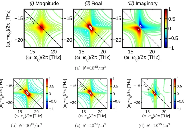
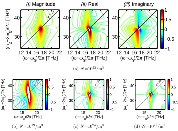
4-7 Calculated two-quantum 2D FTOPT spectrum for a two-level system with local field effects . . . 73
4-8 Calculated 2D FTOPT spectrum for a two-level system with excitation-induced dephasing . . . 75 4-9 Calculated 2D FTOPT spectrum for a two-level system with
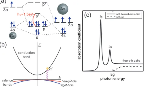
excitation-induced frequency shift . . . 76 5-1 Excitons in a bulk semiconductor . . . 80 5-2 Structure and electron/hole states of a semiconductor quantum well . 81 5-3 Optical transitions and selection rules for quantum well exciton and
biexciton states . . . 85 5-4 GaAs/Al0.3Ga0.7As quantum well absorption spectrum and carrier
den-sity . . . 88 5-5 Schematic of exciton population gratings formed by polarized optical
excitation fields . . . 89 5-6 Pulse sequences for 2D FTOPT spectroscopy . . . 90 5-7 Transients extracted from non-rephasing 2D FTOPT measurements . 91 5-8 Determination of the overall signal-reference phase shift . . . 92 5-9 Feynman diagrams relevant to one-quantum rephasing 2D FTOPT
measurements . . . 94 5-10 Rephasing 2D FTOPT spectra of GaAs quantum wells using co-circularly
polarized excitation fields . . . 95 5-11 Real part of the rephasing 2D FTOPT spectra of GaAs quantum wells
using co-circularly polarized excitation fields compared to results from the modified optical Bloch equations. . . 98 5-12 Rephasing 2D FTOPT spectra of GaAs quantum wells using
cross-circularly polarized excitation fields . . . 99 5-13 Rephasing 2D FTOPT spectra of GaAs quantum wells using
cross-linearly polarized excitation fields . . . 100 5-14 Feynman diagrams relevant to one-quantum non-rephasing 2D FTOPT
5-15 Complex non-rephasing 2D FTOPT spectra of GaAs quantum wells for different excitation polarizations. . . 103 5-16 The effect of an incorrect SLM pixel-to-frequency calibration on the
2D FTOPT spectral magnitude. . . 105 5-17 The effect of an incorrect SLM pixel-to-frequency calibration on the
complex 2D FTOPT spectra. . . 107 5-18 Spectral magnitudes of two-quantum 2D FTOPT measurements for
different excitation field polarizations. . . 110 5-19 Feynman diagrams relevant to two-quantum rephasing 2D FTOPT
measurements . . . 111 5-20 The effect of excitation wavelength detuning on two-quantum 2D FTOPT
measurements. . . 112 5-21 Integrated Two-quantum and emission lineshapes . . . 114 5-22 Real parts of complex two-quantum 2D FTOPT spectra for different
excitation field polarizations. . . 116 5-23 Real part of the two-quantum 2D FTOPT spectrum of GaAs quantum
wells using co-circularly polarized excitation fields compared to results from the modified optical Bloch equations. . . 118 5-24 Carrier density dependence of the biexciton dephasing time. . . 119 5-25 Carrier density dependence of biexciton dephasing times . . . 120 5-26 Carrier density dependence of the dephasing time of two-quantum
sig-nal contributions at 2ωe. . . 121
6-1 Four-wave mixing emission spectrum of Rb vapor at time zero and energy level diagram for Rb. . . 126 6-2 Rephasing complex 2D-FTOPT spectra of Rb vapor . . . 128 6-3 Non-rephasing complex 2D FTOPT spectra of Rb vapor . . . 129 6-4 Non-rephasing complex 2D FTOPT spectra of Rb vapor for the D1
transition only . . . 131 6-5 Two-quantum complex 2D-FTOPT spectra of Rb vapor . . . 133
List of Tables
5.1 One-quantum absorption frequencies in a rotating frame extracted from non-rephasing 2D FTOPT spectra of GaAs QWs. . . 106 5.2 Fitted two-quantum spectral peak positions measured for GaAs QWs
for different excitation field polarizations. . . 115 6.1 Fitted center frequency for peaks in the 2D FTOPT spectra measured
List of Abbreviations
2D FTOPT: Two-dimensional Fourier Transform optical spectroscopy EID: Excitation-induced dephasing
EIS: Excitation-induced frequency (or energy) shift FWM: Four-wave mixing
LFE: Local field effects
MOBE: Modified optical Bloch equations OBE: Optical Bloch equations
QD: Quantum dot QW: Quantum well
SLM: Spatial light modulator X: Exciton-ground-state coherence X2: Biexciton-ground-state coherence
Chapter 1
Introduction
Charged particle correlations play a significant role in determining the coherent op-tical responses of semiconductor nanostructures and assemblies of molecular chro-mophores, which are being considered for new applications in light-harvesting, opto-electronic, and quantum information technologies. The collective electronic states of these materials are formed from linear combinations of the atomic or molecular or-bitals belonging to their individual constituents such that the states are arranged into bands. Absorption of a photon can excite an electron from the filled valence band to the empty conduction band, leaving a positively charged “hole” in the valence band. It is the Coulomb force that mediates the correlation between the two particles and prompts the formation of a new bound state – a quasiparticle known as an exciton.
In semiconductors, the basis for the Wannier-Mott model describing the excitonic bands proceeds from delocalized Bloch wavefunctions. The exciton Bohr radius is large and the electron and hole are loosely bound to each other as they move through-out the material. In contrast, in molecular complexes, the excitonic bands are derived from molecular orbitals such that the Bohr radius of these so-called Frenkel excitons is small and the electron and hole remain strongly overlapped as they move through the complex. It is the delocalization of the atomic/molecular wavefunctions that de-termines the nature and dynamics of the exciton. The spatial extent of the exciton wavefunction can be controlled by modifying the nanoscale structure of the material [1] which provides opportunities for chemists to devise materials with useful optical
and electronic properties.
The optical properties of semiconductors can be tuned by alternately layering two different semiconductor films (with thickness on the order of nanometers) with differ-ent bandgaps or by synthesizing semiconductor particles of nanometer-scale diameter, such that the exciton is confined by a potential energy jump at the boundaries. The tailored optical properties of these so-called semiconductor quantum wells (QWs) and quantum dots (QDs) have proved useful for wide-ranging applications and con-tinue to provide testbeds for fundamental study. For example, coupled QWs are attractive materials for the study of excitonic Bose-Einstein condensates since the exciton lifetime can be controlled with the application of an electric field through the quantum-confined Stark effect [2]. The exciton of a QW embedded in a microcavity can strongly couple to an electromagnetic field to form an exciton-polariton which is also an interesting candidate for solid-state Bose-Einstein condensates [3]. Semi-conductor quantum dots are useful for applications in quantum control and quantum optics since the electron spin decoherence can be manipulated by an optical field [4] and the optical transitions can exhibit interference phenomena (i.e. an Autler-Townes splitting) when driven by a strong optical field [5].
In molecular complexes, the delocalization of the exciton is greatly influenced by the nanoscale arrangement of the chromophores such that the optical properties of conjugated polymers and J -aggregates are strongly dependent on the aggregation state [1]. These materials play important roles in electroluminescent and photovoltaic devices. Their high absorption coefficients enable strong coupling with an optical field, producing luminescent exciton-polariton states when nanolayers of material are sandwiched between the highly reflective surfaces of a microcavity [6]. Integration of inorganic materials, such as quantum dots, which have high fluorescence yields com-pared to organic molecules, into these devices increases their luminescent efficiency [7].
Linear and nonlinear ultrafast spectroscopy techniques [8] are conducive to the study of exciton properties. However, several observations of semiconductor nanos-tructures and molecular chromophore assemblies have shown that correlations between
excitons are significant and that the spectral signatures dependent on their interac-tions may be largely convolved in conventional measurements. The correlainterac-tions give rise to exciton-exciton or exciton-free carrier scattering or the binding of two exci-tons to form a new bound quasiparticle known as a biexciton. The biexciton is often described in terms of a band of two-exciton states with approximately twice the en-ergy of the one-exciton states that can be accessed by absorption of a second optical photon.
In biological light-harvesting complexes, coherently coupled electronic states [9] allow energy-efficient transfer of the photo-excited exciton [10]. Simulations of the coherent dynamics of multiple-electronic correlations such as biexcitons [11] demon-strate that states in the two-exciton manifold may play important roles in natural photosynthetic antenna complexes which appear to have evolved rapid relaxation pathways to avert damage under highly energized conditions. These two-exciton states may also be involved in the coherent control of exciton dynamics [12] in these materials. Absorption into the two-exciton band of a J -aggregate [13] is relevant to determining the size-dependence of optical nonlinearities and understanding processes such as exciton-exciton annihilation in these materials. Simulations of coherently cou-pled exciton states in J -aggregates demonstrate a promising method by which the exciton localization size under different experimental conditions can be investigated [14].
In semiconductor QWs, the effects of exciton-exciton interactions, or “many-body” effects [15], are especially prevalent since Wannier excitons have large Bohr radii. Not only are excitons originating from different valence bands coupled [16], but they may be scattered by exciton or free-carrier populations [17]. Furthermore, the scattering interactions can produce new contributions to the coherent optical response [18]. Biexciton formation also plays a significant role in the coherent optical response of QWs [19, 20, 21, 22]. Two-exciton states have been exploited in coherent control schemes [23] and used to access exciton spin coherences for quantum information processing [24]. In zinc oxide QWs, the biexciton binding energy is strong even at room temperature, making for a stable, strongly absorbing and, therefore, efficient
material for optoelectronic device applications [25]. Similarly, in semiconductor QDs, the complete nonlinear optical response can only be fully simulated when higher-order particle correlations are included [26]. Biexciton states have been exploited for controlling electromagnetically induced transparency [27] for slow-light applications and in an all-optical quantum gate [28] suitable for quantum information processing. Multiply excited states in semiconductor QDs may provide a route to harnessing the extra energy deposited in these materials by the absorption of highly energetic photons [29, 30].
Conventional time- and frequency-domain techniques are indiscriminate with re-spect to many of the re-spectroscopic signatures that would result from the coupling and interaction of excitons. Fortunately, recent efforts in ultrafast infrared (IR) spec-troscopy have allowed the separation of coupled vibrational resonances by adapting methods from two-dimensional Fourier Transform nuclear magnetic resonance (2D FTNMR) spectroscopy. 2D FT spectroscopy uses sequences of pulsed electromag-netic fields to excite coherences in the sample which oscillate during the interpulse delays and whose phases depend on the phase relationships between the fields and the other coherences they generated during previous pulse delays. Coherent super-positions of states that differ by a single quantum, i.e. single-quantum coherences, can be generated through allowed one-photon transitions. Coherent superpositions of states that differ by multiple quanta, i.e. multiple-quantum transitions, are generally nonradiative, but they may be accessed through a sequence of one-photon transi-tions. Optical analogs to the one-quantum and multiple-quantum techniques used in 2D FTNMR and 2D FTIR spectroscopy would permit isolation of exciton coupling and interaction contributions to ultrafast optical (OPT) spectroscopy measurements, since 2D FT spectroscopy methods can reveal correlated coherent motions by provid-ing another frequency axis along which spectral features resultprovid-ing from coupled and interacting excitations can be spread.
While many groups have performed 2D FTIR measurements [31, 32, 33, 34], far fewer have attempted 2D FTOPT spectroscopy. 2D FTOPT measurements require detection of the full signal field through interferometric mixing with a reference field so
that the full optical analog to 2D FTNMR can be realized [35]. While background-free detection of the signal field can be realized by borrowing wavevector-matching tech-niques from optical four-wave mixing (FWM) spectroscopy, the main experimental challenge presented by wavevector definition in the optical regime lies in the difficulty of producing multiple beams of light with pulses whose optical phases are specified and maintained even when the pulses are variably delayed in time-resolved measure-ments. Typically, reflective [36, 37] or diffractive [38, 39] beam-splitting optics are used to produce four distinct beams containing the three excitation fields and the reference field. Glass prisms or delay stages coupled with actively stabilized feedback loops are used to impart the required interpulse delays. With these methods, however, only partial phase stability can be obtained, i.e. the first two fields produced by one beamsplitter are phase-related, as are the third field and reference field produced by another, but no well-defined phase relationship exists between the two pulse pairs. As discussed in subsequent chapters, this is all that is required to perform one-quantum measurements, but full phase stability is a requirement for two-quantum 2D FTOPT measurements since the key element is the two-quantum coherence that is created by the first two pulses and whose phase as well as amplitude is measured by the last two. The Nelson group at MIT has pioneered the use of femtosecond pulse shaping techniques in the temporal [40] and spatial [41] domains for the coherent control of phonon-polaritons [42], which are collective vibrations of a crystal lattice coupled to light. Recently, we showed that spatiotemporal pulse shaping techniques can be used as a platform for various ultrafast spectroscopy experiments [43]. Not only does it offer passive phase stability of all non-collinearly propagating pulses through the use of common path optics, it is also capable of arbitrary waveform generation since in-dependent control of the amplitude and phase profile of each pulse is possible. These characteristics make spatiotemporal pulse shaping ideal for 2D FTOPT spectroscopy experiments, especially when investigation of higher-order correlations or coherent control of the induced response is desired. The spatiotemporal pulse shaping tech-nique for one-quantum and two-quantum 2D FTOPT measurements presented here is distinct from one-quantum 2D FTOPT measurements using collinear phase-controlled
pulses [44] where only a portion of the complex signal field is detected. A recently demonstrated method [45] using only conventional optics also promises full phase stability and full signal field detection, but without the ability to arbitrarily define the excitation waveforms.
In this work, I will present 2D FTOPT measurements using spatiotemporal pulse shaping on semiconductor QWs which reveal exciton coupling and interactions. I will also present the first two-quantum 2D FTOPT measurements on these materials that constitute the first direct observations of biexciton coherences and separation of four-particle correlations from two-four-particle (single-exciton) correlations. Chapter 2 details the pulse sequences used in one-quantum and two-quantum 2D FTOPT spectroscopy. Chapter 3 presents the spatiotemporal pulse shaping technique and discusses its ad-vantages and limitations. The spectral signatures resulting from four-particle corre-lations can be modeled using a phenomenological treatment of exciton interactions which is presented in Chapter 4. Chapter 5 presents 2D FTOPT measurements on ex-citons in semiconductor QWs where the 2D spectral features and complex lineshapes permit direct observation and characterization of four-particle correlations. Chapter 6 presents 2D FTOPT measurement on dense rubidium vapor which contrast with the measurements on semiconductor excitons since the many-body correlations described in Chapter 5 that arise from long-range Coulomb interactions between excitons are absent for excitations in rubidium.
Chapter 2
Theory of 2D Fourier transform
spectroscopy
Nonlinear multidimensional spectroscopic methods permit spreading of congested spectra along multiple time or frequency coordinates, as in nuclear magnetic resonance (NMR) spectroscopy [46], thereby enabling quantitative determination of couplings, anharmonicities, relative dipole orientations, and dynamical processes that depend on them. These unique abilities have been elegantly demonstrated in many experiments over the past several years using coherent 2D spectroscopy with ultrashort pulses in the mid-infrared [47, 48, 49, 50, 51] and in the visible or near-infrared [52, 9, 53, 44] spectral ranges. In this chapter, I will discuss the coherent dynamics measured in 2D FTOPT spectroscopy and introduce the sequences of optical field interactions that are used to probe these dynamics by relating 2D FTOPT measurements to one-quantum and multiple-quantum measurements used in 2D FTNMR.
2.1
Coupled two-particle correlations and one-quantum
techniques
In NMR spectroscopy, 2D FT techniques are useful for studying correlated spin re-sponses. In 2D FTNMR, a series of radiofrequency (RF) magnetic fields are used
to manipulate an ensemble of nuclear spins oriented in a dc magnetic field polarized perpendicular to the RF fields. The first RF field, referred to as a π
2-pulse because it moves the net magnetization vector by 90o from the z axis to the x-y plane, inducing
nuclear spin coherences that are described quantum mechanically as superpositions between | +i and | −i spin states oriented along and against the dc field and that constitute an ensemble of radiating magnetic dipoles. In the simplest form of NMR spectroscopy, the resulting “free induction decay” detected by a magnetic coil is used to determine the spin precession frequency, ωs, and dephasing rate, γs. However,
in a 2D FTNMR measurement a second RF field (also π
2) applied after a variable delay, τ1, aligns the dipoles to the axis parallel with the dc field. During the following period, τ2, a through-space dipole-dipole interaction causes an exchange of the mag-netization. Then a third RF field (also π
2) restores the nuclear spin coherences whose radiation is sensed by a magnetic coil during the final period, t. Subsequent 2D FT of the signal with respect to τ1 and t yields a 2D FTNMR spectrum which shows cross-peaks, indicating that a magnetic dipole took on two different spin precession frequencies during the first and final time periods due to the magnetization exchange that occurred during τ2.
From the preceding description of coupled nuclear spins, it is evident how 2D FT spectroscopy can be used to separate coupled vibrational and electronic coherences using ultrafast laser pulses in the infrared (IR) [54] and optical (OPT) [55] regimes, respectively, by combining familiar four-wave mixing (FWM) spectroscopy techniques with interferometric detection of the signal field. One important difference between RF and IR/OPT fields is that, in 2D FTNMR, the RF wavelengths far exceed the sample dimensions, and the sample is surrounded by the coils that deliver the fields and measure the responses. In this limit, the RF field frequencies and polarizations are important but their propagation directions are not. In contrast, in 2D FTIR and 2D FTOPT measurements the sample is large compared to the wavelength, and the fields are delivered to the sample and radiated from it in the form of coherent light beams with well-defined propagation directions, i.e. wavevectors. The key opportunities afforded by wavevector definition lie in the use of a non-collinear geometry of the
beams at the sample and the specification of the pulse time-ordering to select and sharply limit the contributions to the measured signal that is radiated from the sample as a coherent beam in a well-defined direction. If the three ultrafast excitation fields,
~
EA, ~EBand ~EC, arrive at the sample with distinct wavevectors ~kA, ~kBand ~kC, then the
FWM signal field, ~ES, will radiate in the direction given by the wavevector-matching
condition: ~kS = ~kA+ ~kB− ~kC, as shown in Fig. 2-1.
→ → EA(kA) → → ER(kR) E→ →B(kB) → → EC(kC) → → → → → ES(kS= kA+ kB - kC)
(a)
(b)
→ → EA(kA) → → EB(kB) → → EC(kC)S1
S2
S3
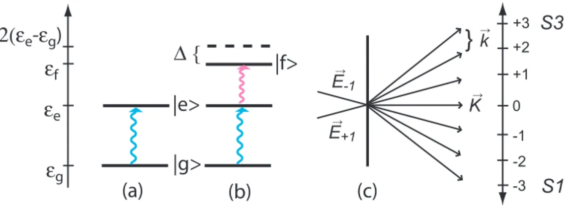
Figure 2-1: As in degenerate FWM spectroscopy experiments, 2D FTOPT can benefit from the use of non-collinear excitation fields arranged in the BOXCARS geometry (a) to spatially isolate three types of signals described as S1, S2, S3 (see main text). The spatial positions of the signals relative to the excitation fields are shown in (b) for the time-ordering of the fields where ~EC is second to arrive at the sample. The
spatial position of the signals will change if the time-ordering of fields is changed, such that the S1(S3) signal propagates to the fourth corner of the box if field ~EC
arrives first(last). A reference field, ~ER, which propagates in the same direction as
the signal field, may be used for interferometric detection of the signal.
Two important types of one-quantum 2D FTOPT signals can be spatially isolated using this geometry just by changing the time-ordering of the “conjugate” field, ~EC
(so-called because it contributes its backward-propagating spatial and temporal com-ponents to the signal), such that it arrives first or second at the sample. In nonlinear spectroscopy terminology, these pulse sequences are named S1 and S2.
In the S1 pulse sequence, depicted in Fig. 2-2(a), field ~EC arrives first to generate
an exciton coherence in the sample, and after a variable delay, τ1, interaction with field ~EA produces an excited state population in a transient grating pattern with
wavevector ~kA− ~kC. The population grating diffracts the field ~EB, incident at the
phase-matching or Bragg angle, to yield the coherently scattered signal ~ES, which
evolves during the final time period t. The last excitation field ~EB also reverses the
temporal phase of the coherences that evolved during τ1 such that the decay of ~ES(τ1) yields the homogeneous dephasing time, since any inhomogeneous dephasing due to local variation in the frequency is reversed due to the “rephasing” induced by ~EB.
Similar to the case of nuclear spins, if there are multiple electronic transitions excited at different frequencies within the spectral bandwidth of the pulses, then multiple coherences will be rephased in the signal field, and if two coherences are coupled, then the signal field components at each frequency will be modulated at the other frequency. The full signal field, ~ES(τ1, t), is measured using interferometric methods with a reference field ~ER that propagates collinearly with the signal field direction,
i.e. ~kR = ~kS, and subsequent 2D Fourier transformation of the signal field yields a
two-dimensional spectrum, S(ω1, ω), where coherences that evolved during τ1(t) are spread along the ω1(ω) coordinate. The 2D spectrum shows diagonal peaks due to each individual coherence and off-diagonal cross-peaks that reveal the coupled exciton coherences. All of the peaks will be elongated along the diagonal and the linewidth of the peak antiparallel to the diagonal yields the homogeneous dephasing time.
time
t
t
1t
2 → →E
A(k
A)
E
→ →B(k
B)
→ →E
C(-k
C)
E
→ →R(k
R)
→ → → → → →E
S(k
S=
-k
C+
k
A+
k
B=
k
R)
(a) Rephasing (S1)time
t
t
1t
2 → →E
A(k
A)
E
→ →C(-k
C)
E
→ →B(k
B)
→ →E
R(k
R)
→ → → → → →E
S(k
S=
k
A-
k
C+
k
B=
k
R)
(b) Non-rephasing (S2)Figure 2-2: Pulse sequences for one-quantum 2D FTOPT spectroscopy. In the S2 pulse sequence, depicted in Fig. 2-2(b), field ~EAarrives first to generate
electronic coherences followed by field ~EC which interacts to form the excited state
population grating. In this case, the last field ~EBdoes not reverse the temporal phase
the S1 case, multiple coherences will be present in the signal field if the two coherences are coupled, such that 2D Fourier transformation of the signal shows diagonal and off-diagonal peaks. However, these peaks will not be elongated along the off-diagonal since the S2 pulse sequence is not able to eliminate inhomogeneous broadening from the sample. For both S1 and S2 measurements, the interpulse delay τ2 can be scanned in order to obtain the lifetime of the excited state population. The off-diagonal features of the one-quantum 2D spectra can be monitored as a function of τ2 which may reveal how electronic energy is coherently transferred between excitonic states.
Detection of the full signal field in these measurements allows separate exami-nation of the real and imaginary parts of the sample response, revealing induced dynamics that are both absorptive and dispersive in character. In both the S1 and S2 cases, the complex parts of the 2D spectra are not purely absorptive or dispersive, un-like the real and imaginary parts of a 1D FTNMR spectrum. In the 1D measurement, the real part is purely absorptive and can be entirely negative-going, which indicates absorption, or entirely positive-going, which indicates emission. The imaginary part of the 1D spectrum is dispersive and indicates a change in phase, rather than ampli-tude, of the signal field, and exhibits a node at the resonance frequency, such that, for positive dispersion, the slope of the lineshape remains positive with respect to increasing frequency. See Section 4.2 for further examples. On the other hand, the complex S1 and S2 2D lineshapes exhibit a “phase twist” such that the real part of the 2D spectral peaks, while still largely absorptive, have some dispersive characteristics. This is due to the fact that the 2D Fourier transform of ~ES(τ1, t) takes into account both the positive and negative values for τ1 and t, such that Fourier transformation along either dimension separately yields an imaginary dispersive lineshape and sub-sequent 1D Fourier transformation along the opposite dimension mixes the dispersive lineshape into the total real 2D lineshape. The phase twist can be eliminated by correct addition of the real parts of the rephasing and non-rephasing 2D spectra [56].
2.2
Four-particle correlations and two-quantum
tech-niques
In a single-pulse NMR measurement, the detected free induction decay is modified according the shielding of the magnetic dipole by the electron cloud and the coupling of the dipole to the dipolar field of another nucleus attached by a chemical bond. Based on this interpretation of a nuclear spin in a local magnetic field, it is straight-forward to obtain molecular structural information when the sources of the local fields are limited. However, the spectra can become intractable for a large molecule. Al-though the one-quantum 2D FTNMR measurements described above are much more powerful than a simple single-pulse NMR measurement, since coupled nuclear spin co-herences can be spread out along two frequency axes, the 2D spectra can still become too crowded for very large molecules like proteins and other polymers. However, in multiple-quantum NMR techniques, the response from multiple spins correlated through the aforementioned dipolar interactions is modulated by far fewer magnetic field contributions. Therefore, multiple-quantum techniques offer yet another degree of refinement by which signal contributions from congested one-quantum spectra can be isolated.
High-order nuclear spin coherences have been isolated and observed through multiple-quantum techniques [57, 58] used in 2D FTNMR spectroscopy. Multiple-multiple-quantum coherences do not radiate but they can be generated and probed in successive steps. First, each of the two RF fields, which may or may not be separated in time, induces a macroscopic spin coherence in the sample (a precession of the net magnetic moment) described quantum mechanically as a coherent superposition between the | +i and
| −i spin states which evolves with the spin precession frequency ωs. Neighboring
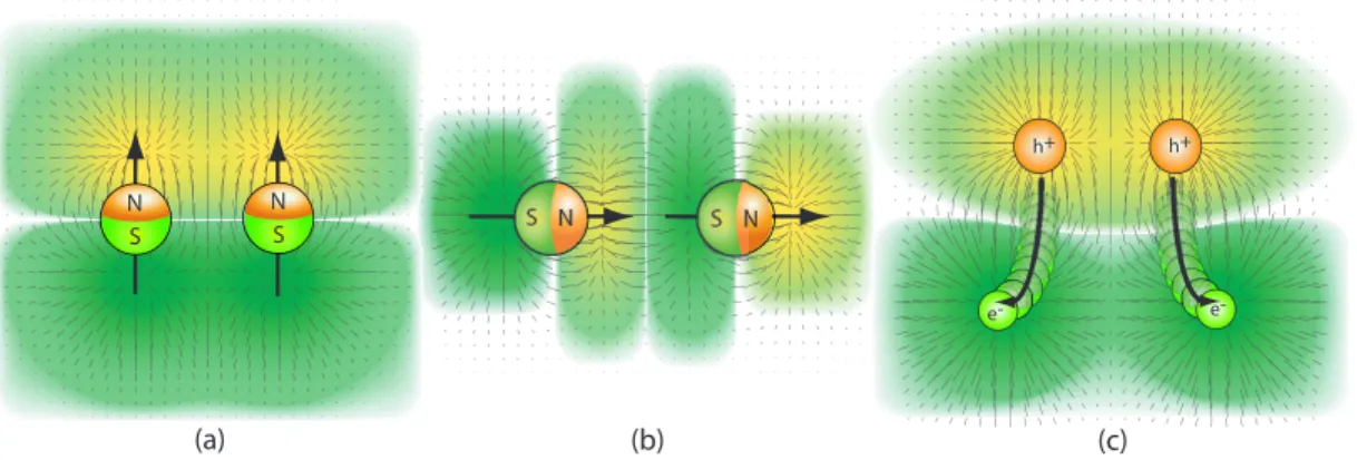
spins are influenced by each other’s magnetic moments through dipolar interactions, and the interaction strength is different when the precessing moments are aligned parallel or perpendicular to the direction between the two nuclei, as depicted in Fig. 2-3(a) and (b). The interaction – and the response of the precessing spins to it – thus has a component that oscillates at twice the precession frequency, 2ωs. This
two-quantum coherent superposition of the | - - i and | + + i spin states has no
net magnetic moment, and therefore is non-radiative and cannot be sensed directly. However a third field, phase-coherent with the first two fields and delayed by a tem-poral period τ2, produces a new one-quantum spin coherence whose free induction decay is measured. The amplitude and phase of the resulting signal emitted dur-ing time t after the third field depend on the phase relationships between the RF fields and the one- and two-quantum coherences they generated. A 2D FT of the complex signal, S(τ2, t), yields a 2D spectrum, S(ω2, ω), where groups of measured spin coherences (appearing along the emission frequency coordinate) sharing the same multiple-quantum coherence frequency along the ω2 coordinate originate from equiv-alent pairs of nearby nuclei, and from this information the skeleton of even a large protein can be constructed. The multiple-quantum technique allows further simplifi-cation over conventional one-quantum spectra. Multiple-quantum techniques in NMR also permit the selection of correlations between spins on different molecules in a liq-uid mixture [59], providing information about liqliq-uid state structural dynamics [60].
N S S N N S N S h+ h+ e- e-(a) (b) (c)
Figure 2-3: Interactions between two nuclear spins oriented (a) perpendicular and (b) parallel to the vector between the two nuclei. (c) Interactions between two electron-hole pairs.
A two-quantum 2D FTOPT signal can be isolated by again changing the time-ordering of the fields such that ~EC arrives last at the sample. Analogous to the
exciton frequency, ωe. The coherence can be described quantum mechanically as a
superposition between the exciton wavefunction, | Xi, and ground state wavefunction,
| 0i, which specifies the absence of any electronic excitation in the system. Two
electrons’ trajectories during one-fourth of a coherence cycle are suggested by the black arrows in Fig. 2-3(c). As the nearby electrons move away from their parent holes, the screening forces provided by the holes are diminished and the electrons are more strongly repelled from each other. This occurs twice during each cycle, so the interparticle forces and the particle responses to them oscillate at 2ωe.
Unlike the spin case, exciton correlations involve two pairs of real particles, and the holes also are alternately repelled and attracted at 2ωeas the screening between them
provided by the electrons varies at that frequency. These correlated interactions may give rise to measurable changes in the exciton energy εeand dephasing rate γe. Nearby
excitons also may interact through their locally radiated fields, further modulating each others’ motions at 2ωe.
Furthermore, the electron-hole pairs can adopt new time-averaged configurations, forming a biexciton state, | X2i, which is a bound quasiparticle formed from two exciton states, whose energy is minimized at a value lower than twice the exciton energy. As in the spin case, the biexciton-ground state coherence, and the other two-quantum coherences described above, which evolve during time period τ2, are non-radiative. However, they can be detected through the action of a third field, ~EC,
that induces transitions to one-quantum coherences whose signals, radiated during t, depend on the phase relationships between the first two and third fields.
time
t
t
1t
2 → →E
A(k
A)
→ →E
B(k
B)
→ →E
C(-k
C)
E
→ →R(k
R)
→ → → → → →E
S(k
S=
k
A+
k
B-
k
C=
k
R)
Figure 2-4: Pulse sequence used for two-quantum 2D FTOPT spectroscopy measure-ments.
The scenario described above shows how distinct biexciton and other two-quantum signals could be observed through an optical analog to two-quantum 2D FTNMR, i.e. two-quantum 2D FTOPT using the pulse sequence, also named S3, depicted in Fig. 2-4. In contrast to multiple-quantum nuclear spin coherences whose fundamental properties are well understood and whose measurement is conducted mainly to sim-plify complicated spectra, multiple-quantum optical coherences are of strong interest because they provide access to “dark” states whose properties and behavior are gen-erally poorly understood and whose understanding may reveal much about high-order correlations in condensed matter, as described in Chapter 1.
However, performing these experiments in the optical regime requires that all the excitation fields and the reference field, used for interferometric detection which yields the full complex signal (rather than just its intensity), have controlled phase relationships. Combining this requirement with the key advantage of background-free detection of the full signal afforded by wavevector-matching of the optical ex-citation fields presents challenges because it means that phase relationships must be maintained among multiple noncollinear light fields that intersect at the sample. While two-quantum 2D FTIR spectroscopy of molecular vibrational overtones has been demonstrated in the infrared spectral region [61, 62, 63], where the wavelength is long enough that the phases of the IR fields in distinct beams can be maintained without extraordinary measures, a comparable measurement in the visible region is far more demanding. In the Chapter 3, I will describe an experimental technique for fully coherent 2D FTOPT spectroscopy, spatiotemporal pulse shaping, which ad-dresses these challenges.
Chapter 3
Experimental methods
3.1
Introduction
Pulse shaping of ultrafast optical fields provides a unique and robust platform for performing many types of ultrafast spectroscopy measurements [43] and coherent control experiments [64]. In general, modulation of the temporal and spatial profile of a femtosecond laser pulse is achieved through filtering of the amplitudes and phases of its frequency and wavevector components. This calls for optical components that can discriminate between the different Fourier components of the pulse. Typical temporal pulse shaping setups involve diffractive or refractive elements, such as gratings or prisms, which can impart a different wavevector to each of the frequency components of the broadband laser pulse, and a focussing element, such as a lens or curved mirror, which focus the frequency components to different points in space at the focal plane. The phase and/or amplitude filtering element, called a spatial light modulator (SLM), is placed at the Fourier plane of the focusing element. The phase and amplitude profile imparted on the incoming waveform in frequency space, Ein(ν),
can be treated mathematically as a transfer function, such that the output waveform is defined in the frequency domain as
or equivalently in the time domain, via the convolution theorem,
eout(t) = m(t) ∗ ein(t). (3.2)
SLMs with varied principles of operation have been devised [65]. The most ubiq-uitous are liquid crystal and acousto-optic based SLMs where the refractive index of the material can be controlled electrically [40, 66, 67] or by the oscillating mechan-ical pressure of a sound wave [68, 69], respectively. Mirror-based SLMs, where the positions of separate elements of the mirror are controlled through piezoelectric [70] or MEMS-based [71, 72] actuators, are also common.
Fully coherent 2D FTOPT afforded through spatiotemporal pulse shaping, which creates the four non-collinearly propagating optical fields from a single laser pulse in a single beam, and controls independently their interpulse delays, has both advantages and limitations. The key advantage for 2D FTOPT spectroscopy is that the phase relationships between features of the shaped waveform are passively stabilized through the use of common path optics, therefore eliminating the need to track or actively stabilize the phase offsets. Furthermore, as discussed below, the coherences detected during the first and second pulse delays, τ1 and τ2, respectively, are shifted into the rotating frame such that the reference frequency is defined by user. Also, the SLM can arbitrarily shape the phase and amplitude of the incoming fields.
The biggest limitation of spatiotemporal pulse shaping is that the output wave-forms cannot be delayed beyond a certain maximum value in time. This is due to the fact that the phase profile applied in the frequency domain is not infinitely sampled. In other words, there is a minimum frequency sampling interval, δν, over which the applied phase is defined, which is determined in part by the frequency resolution achieved by the diffractive and refractive optical elements discussed above and the number and physical size of the SLM pixels. The maximum achievable time delay is easy to determine. By simple Fourier transform relationships, one can show that a temporal delay of the pulse envelope, τ , corresponds to a linear change in phase with respect to the frequency components of the pulse, φ(ν), such that φ(ν) = −2π(ν−νc)τ ,
where νcis the carrier frequency of the pulse. This expression can be restated in terms
of its slope, and therefore, the minimum frequency sampling interval, such that
τ = − δφ
2πδν. (3.3)
Since the maximum phase change is 2π, the maximum time delay of the pulse envelope that can be achieved is simply 1/δν. Furthermore, the intensity of the pulse will be modulated as the pulse is delayed, which imposes a minimum linewidth that will be convolved with the linewidth of the measured spectral features along the ω1 and ω2 coordinates. However, this distortion can be decoupled from the measurement as discussed in Section 3.3.3.
Since many of the experimental details regarding spatiotemporal pulse shaping, such as frequency-to-pixel calibration, phase change versus applied voltage calibra-tion, and output waveform characterization have been published elsewhere [43, 73, 74], in this chapter I will discuss only the features of spatiotemporal pulse shaping that are directly relevant to 2D FTOPT measurements in addition to the optical setup.
3.2
The Multidimensional Optical Spectrometer
The optical components for the Multidimensional Optical Spectrometer, shown in Fig. 3-1, can be divided into three main parts: diffractive beam shaping, spatiotem-poral pulse shaping, and spectral interferometry of the signal field. The main optical elements are summarized here. Diffractive beam-shaping and diffraction-based pulse shaping are discussed in further detail in Sections 3.2.1 and 3.2.2, respectively. As shown in Fig. 3-1, the beams containing the three pulsed fields, ~EA, ~EB and ~EC,
used to excite the coherent third order response in the sample and the reference field, ~ER, used to interferometrically detect the resulting the signal, are generated,
via diffractive beam shaping, from a single pulse in a single Gaussian beam from an unamplified Ti:sapphire laser with an energy of 3 nJ/pulse and a beam diameter of approximately 2 mm. The static diffractive optic has a square lattice pattern which
DO SL1 BS SF QW SL4 G CL 2D SLM → → ES(τ1,τ2,t)+ER(t) → EA → EC → EB Α(ω) φ(ω) f f SL3 SF SL3 → →
|
ES(τ1,τ2,ω)+ER(ω)|
2Figure 3-1: Components of the Multidimensional Optical Spectrometer. The labeled components are as follows: (SL1) 10 cm focal length spherical lens, (DO) static diffractive optic, (BS) 50/50 beamsplitter, (G) gold 1400 grooves/mm diffraction grating, (CL) 12.5 cm focal length cylindrical lens, (2D SLM) two-dimensional liquid spatial light modulator, Hamamatsu PAL-SLM X8267, (SL3) 80 cm focal length spherical lens, (SF) spatial filter, and (SL4) 15 cm focal length spherical lens. The optics are arranged in an imaging geometry (see main text). The inset depicts the phase pattern used for diffraction-based pulse shaping.
diffracts most of the input laser beam power into four beams, which pass through a beamsplitter and into the pulse shaper consisting of a grating, cylindrical lens and 2D liquid crystal spatial light modulator. The frequency components of the four beams are dispersed horizontally across four distinct regions of the SLM where their am-plitudes and phases are controlled through diffraction, as detailed below. Then the frequency components are recombined at the grating, yielding the four fully phase-coherent, temporally shaped fields, ~EA, ~EB, ~EC and ~ER. The fields are reflected by
the beamsplitter and focused through a spatial filter and then into the sample. The signal emerges from the sample in the wavevector-matching direction, collinear with
~
ER, and the superposed fields are directed into a spectrometer. The amplitude and
phase of the signal are then obtained through spectral interferometry [75].
One drawback of this setup is that much of the input laser beam power is lost. Approximately 50% of the beam power is lost to higher diffraction orders in the diffractive beam shaping portion of the apparatus. Another 75% is lost because of two passes through the 50/50 beamsplitter. The diffraction grating is approximately 90% efficient and 80% of the beam power is retained after the spatial filter. There-fore, the overall efficiency of the setup is approximately 10%. Improvement has been demonstrated by taking advantage of the slight displacements of the shaped pulses from their incident beam paths as they emerge from the pulse shaper. The beam-splitter can be eliminated, the incident beams sent directly into the pulse shaper, and the displaced beams directed to a high reflector and into the rest of the setup. In this manner the 75% loss due to the beamsplitter is avoided.
3.2.1
Diffractive beam shaping
Diffractive beam shaping is depicted in Fig. 3-2(a). The laser output is focused into a static diffractive optic using a 10 cm spherical lens. The diffractive optic was constructed by mounting back-to-back two separate transmission gratings of equal groove spacing which could be rotated independently. The net result is a diffractive optic that has a square lattice pattern with a feature spacing of 9 µm and a feature depth of 400 nm which permits the most efficient diffraction of the beam into the
±1 diffraction orders. A second 10 cm lens collimates the diffracted beams so that
the final beam pattern consists of four beams arranged on the corners of a square approximately 1 cm on a side. This is the familiar “BOXCARS” geometry used in many FWM experiments. The entire BOXCARS beam pattern is rotated approxi-mately 25◦ so that after diffraction by the grating, none of the dispersed frequency
components belonging to the four fields are overlapped on the surface of the 2D SLM. Approximately 50% of the input beam power is dispersed into the four major 1st order
diffracted beams. The zeroth and higher diffraction orders are blocked after the 2D pulse shaper. SLM SL1 SL2 SL3 DO Sample f0 f0 f2 SF f1 f1 SL4 f2 f3
(a) Diffractive beam shaping
SLM SL3 SL5 Mask SL6
Sample
f1 f1 f2 f2 f3 f3
SF
(b) Real-space beam shaping
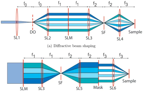
Figure 3-2: Diffractive (a) versus real-space (b) beam shaping in an imaging geometry. The optical elements depicted in (a) are equivalent to the elements with the same labels in Fig. 3-1. In (b), the spherical lens, SL5, is involved in imaging the 2D SLM phase pattern to the spatial mask (see main text).
Spatiotemporal pulse shaping was first used for phase-coherent FWM without a diffractive optic to separate the incident light into four beams [43], which is depicted in Fig. 3-2(b). Instead, a single beam was sent into the pulse shaper, and four distinct regions of the SLM were used to produce four shaped outputs. These were incident onto a spatial mask with four holes placed at the corners of a square pattern, so four
beams, one from each distinct region of the SLM, emerged for use in the BOXCARS geometry. However, the spatial filtering by the holes blocked the great majority of the light, yielding poor throughput, and diffraction and scattering off of the edges of the holes added significantly to experimental noise. Beam shaping by diffraction increases the efficiency of the setup by an order of magnitude, produces outputs with Gaussian spatial profiles, and minimizes cross-talk between pulses generated from nearby regions on the SLM or from aperture edges. The beam pattern can also be easily reconfigured if the static diffractive optic is replaced with an adaptive element, such as another 2D SLM. Any pulse-front tilt imparted to the optical pulses by the diffractive element is eliminated at the sample if the beams are properly imaged from their point of generation to the sample [76].
3.2.2
Diffraction-based spatiotemporal pulse shaping using a
2D SLM
The amplitudes and phases of the frequency components of the four beams dispersed horizontally across four distinct vertical regions of the SLM are controlled through diffraction [77]. The SLM is ordinarily a phase-only device, that is, the liquid crystal rotation at any pixel is used to shift the phase of light that arrives there. Diffraction-based shaping allows control of the amplitudes as well as the phases of the separated spectral components. This is achieved with a 2D SLM by constructing a sawtooth grating pattern in the vertical direction with amplitude A(ω), spatial phase φ(ω), and period d, (see Fig. 3-3(b) and inset of Fig. 3-1) for each of the horizontally separated frequency components of each of the four beams. The amplitude and phase of the diffracted light for each selected frequency component, E(ω), are controlled by the amplitude and spatial phase of the corresponding sawtooth grating pattern, such that
E(ω) = exp[i2πφ(ω)]sinc[π(1 − A(ω))] (3.4) where φ(ω) = ∆
d and ∆ is the vertical displacement of the sawtooth grating pattern.
SF ER EB EA EC BS G CL 2D SLM SL3 ω(x) ω(x)
φ
R(ω)
φ
A(ω)
φ
B(ω)
φ
C(ω)
ω
0 SLM surface y f f y f f φmax=2πA ∆ d 1/d 2/d n/d 0 (a) (b)Figure 3-3: Illustration of the spatiotemporal pulse shaper operating in diffraction mode. The separated frequency components of the broadband pulses are projected onto the surface of the 2D SLM, shown in (a), effectively dividing it into four dis-tinct horizontal regions. Within each region, each dispersed frequency component is diffracted by a sawtooth phase pattern, which is shown in (b) as a red dashed line. The phase for one selected frequency component is kept fixed for all four regions, which defines the reference frequency ω0 (see the discussion in Section 3.3.1).
grating pattern and its spatial phase for each spectral component of each pulse. A phase that increases (decreases) linearly as a function of frequency yields a negative (positive) pulse envelope temporal delay. In the example depicted here, fields ~EA
and ~EB are unmodulated, i.e. all their frequency components have the same phase,
yielding pulses that are unshifted from t = 0. Fields ~EC and ~ER are temporally
shifted from t = 0 by different amounts. Clearly, the SLM can be used to control the temporal delays of any of the pulses without the need for delay stages or variable-thickness elements (wedges) in the beam paths.
Recalling Eqn. 3.3, it follows that the minimum time delay achieved for the output waveforms is related to the minimum phase change, which depends on the how many independent phase values can be distinguished by the SLM. In the case of diffraction-based pulse shaping, the minimum phase change is the minimum vertical displacement of the sawtooth grating pattern. This pattern is defined in terms of the number of SLM pixels used to define d, the sawtooth period, and therefore the sampling interval for the sawtooth grating pattern is one SLM pixel. For the PAL-SLM X8267, which has 768 pixels along its vertical dimension, typically 12 pixels are used to define d, therefore the minimum phase change is 2π1
12 radians. For the specific grating-lens pair used in this optical setup, δν=0.05 THz. Thus the minimum time delay is 1.67 ps which is far too large a step size for most ultrafast spectroscopy measurements. What is done in practice is that the linear phase profile (with respect to frequency) is oversampled in the frequency domain, such that several columns of pixels are binned together and the respective sawtooth phase profiles have the same vertical displacement. With respect to Eqn. 3.3, the binning of columns of pixels increases the frequency sampling interval, which in turn, allows a smaller minimum time delay for a fixed minimum phase change. For example, if the columns of pixels are binned into 4 groups of 192 pixels each, then the minimum time delay is approximately 9 fs.
Diffraction-based pulse shaping also discriminates against the pulse replica created due to imperfections in the pixel shape of the SLM which mar the shaped output de-livered by standard reflection-based pulse shaping [41]. After the spectral components
have been diffracted from the SLM and recombined into the user-defined temporal waveforms, the focusing of the beams through the spatial filter eliminates these repli-cas and the de-selected frequency components from the final waveforms used for the experiment. However, the variation of the shaped output as a function of delay must be determined carefully prior to successful spectroscopic measurements. The main distortion is the decrease, or “roll-off” in the intensity of the pulse as it is delayed, which is due to the pixelated nature of the SLM and the smooth shape of the pixels [73, 74]. Pulse intensity roll-off is discussed in more detail in Section 3.3.3.
3.3
2D FTOPT spectroscopy using SLM-delayed
pulses
Here I will discuss in detail several of the advantages, such as passive phase stability, rotating frame detection, and phase cycling and phasing of the signal, and limita-tions, such as pulse intensity roll-off, of the spatiotemporal pulse shaping technique in relation to 2D FTOPT spectroscopy.
3.3.1
Rotating frame detection
The pulse shaper permits the relative delay times between pulses to be varied while maintaining the relative optical phase relationships constant. This is accomplished by selecting a reference frequency ω0within the spectral bandwidths of the pulses and then varying the slope dφdω of the linear phase sweep in the SLM pixel pattern to change the relative pulse envelope delays while keeping the phase of the selected reference frequency constant. Thus, the amplitude and phase of the waveform generated by the SLM for one of the incident pulses can be written in the frequency domain and time domain as
E(ω) = A(ω)exp[i(ω − ω0)τ − iφ(0)] (3.5)