Demonstration of methods for analytical measurement of natural circulation flow in EBR-II

MASSACHUSETTS INSTITUTE

OF TECHNOLOGY

KUCLEAR ENGIWEI%

REMING

ROOM Mi

DEMONSTRATION OF METHODS

FOR ANALYTIC MEASUREMENT

OF NATURAL CIRCULATION FLOW IN EBR-II

R. J. Witt and J. E. Meyer

February, 1986

r~t WI

r~r~

REATh~

MITNE-270

R00M

u

ML

Department of Nuclear Engineering

Massachusetts Institute of Technology

Includes MIT technical contributions from

J. I. Choi, D. D. Lanning, J. E. Meyer, A. L. Schor,

R. J. Witt and R. D. Wittmeier

DEMONSTRATION OF METHODS

FOR ANALYTIC MEASUREMENT

OF NATURAL CIRCULATION FLOW IN EBR-II

R. J. Witt and J. E. Meyer

February, 1986

Final Project Report

U. S. Department of Energy

Breeder Technology Program

Division of Educational Programs

Argonne National Laboratory

ABSTRACT

Two analytic models have been developed for inferring the flowrate in the EBR-II reactor during natural circulation. The first model results in an analytic measurement of flow which relies mainly on thermocouple readings from the Data Acquisition System and which is performed in two steps. In the first step, which is executed before the reactor is brought to power, ratios of temperature rise across pairs of subassemblies are calculated as a function of total reactor flow and power. These ratios have been found to be relatively weak functions of the total power level, which is attributed to the strong transverse conduction between subassemblies present at low flows. In the second step, which takes place on-line during natural circulation, ratios of temperature rise across pairs of subassemblies are calculated from the Data Acquisition System thermocouple readings, and the flow is inferred from the tables generated in the first step. Because of the weak dependence on power level, a reasonable value of flowrate may be inferred from tables generated at a single representative level.

The second model is based on a transient heat balance of the reactor after shutdown. This model requires the power history of the reactor prior to shutdown as well as the inlet and outlet sodium temperatures. The decay heat after shutdown is calculated using the

ANS Revised Standard. Two independent estimates of the flow are obtained by using

different sets of thermocouples to calculate the outlet temperature.

Comparisons of the individual analytic measurements with direct flow measurements are presented for the recent SHRT tests 2, 3, 4, 11 and 12. A validated flow estimate is then obtained from a weighted average of the individual analytic measurements and the direct flow measurement and compared with the direct flow measurement. The results indicate generally good agreement between the individual analytic measurements and the direct flow measurement, although there are instances when the agreement is poor. Possible reasons for the discrepancies are discussed. The weighted average of the individual flows,

however, consistently provides an excellent estimate of the natural circulation flow.

ACKNOWLEDGEMENTS

This work was supported by Argonne National Laboratory - U. S. Department of

Energy. We appreciate the continuing support offered by R. W. Lindsay (EBR-II). The assistance of P. R. Betten (ANL) for the preparation of the SHRT data tape was an essential ingredient and is gratefully acknowledged.

Table of Contents

Abstract 2

Acknowledgements 3

Table of Contents 3

1. Introduction 4

2. Assembly Heat Balance Model 5

2.1 Tabulation of Temperature Rise Ratios 5

2.2 Basis for Governing Equations 6

2.3 Governing Equations 7

2.4 Solution Procedure 10

3. Transient Heat Balance Models 14

3.1 Expressions for Decay Heat 14

3.2 Stored Energy Removal 16

3.3 Transient Heat Balance Equation 16

4. Signal Validation Techniques 17

5. Testing the Methods 18

6. Summary and Conclusions 23

Appendix A - Newt on/iRaphson Method 25

Appendix B --Analytic vs. Direct Measurements 28

Appendix C - Temperature Gradient Near Row Six 38

Appendix D - Inlet and Validated Outlet Temperatures 41

DEMONSTRATION OF METHODS FOR ANALYTIC MEASUREMENT

OF NATURAL CIRCULATION FLOW IN EBR-II

R. J. Witt and J. E. Meyer February, 1986

Includes MIT technical contributions from

J. I. Choi, D. D. Lanning, J. E. Meyer, A. L. Schor,

R. J. Witt and R. D. Wittmeier

1. Introduction

The operator of a nuclear power plant is supplied with an extraordinary amount of information from plant sensors. In some instances he must choose between conflicting results from redundant or related sensors; this situation should obviously be avoided, especially when the wrong choice could result in serious consequences.

One way to avoid this situation is to intercept and validate the information provided

by the plant Data Acquisition System (DAS) before the information is sent to the operator.

This may be accomplished by constructing analytic measurements to supplement direct measurements, and then submitting all measurements to a fault detection and isolation (FDI) algorithm. After processing the information, the FDI sends a validated estimate to the operator. Techniques of signal validation were applied to the EBR-II reactor flowrate in the forced flow regime in work performed by the Charles Stark Draper Laboratory

(1].

In addition, analytic measurement techniques were developed for the EBR-II reactor in the natural circulation regime and compared with direct measurements for Test 8A

[2).

After refining these analytic techniques, a signal validation architecture was developed to obtain a validated flow estimate from both the analytic and direct flow measurements. Comparisons between the individual analytic and direct flow measurements (as well as comparisons between the validated flow estimate and the direct flow measurement) were made for Test 8A after these modifications

[3).

The purpose of the present work is to review

the analytic models and make similar comparisons for several of the recent Shutdown Heat Removal Tests (SHRT's).

2. Assembly Heat Balance Model.

The first method of inferring the flowrate is called the Assembly Heat Balance Model (AHBM) and is based on the flattening of the inter-assembly temperature profile at low flows. As the total flow within the reactor decreases, the elevation pressure drop becomes comparable to, and then greater than, the frictional pressure drop. Flows within hot channels increase, and those within cool channels decrease, so that the total pressure drop across each subassembly is the same. The degree to which the inter-assembly profile is flattened depends on the total flow and power levels in the reactor; hence, the flowrate can be inferred from measurements of relative temperature rise across different parts of

the reactor.

The Experimental Breeder Reactor-I (EBR-II) is equipped with thermocouples that allow such inferences to be made. Such thermocouples are located in the lower plenum and in the outlet flow paths of several (typically ten) subassemblies. Ratios of temperature rise across pairs of subassemblies are then calculated; usually, each "hot" subasembly (typically five) is paired with each "cold" subassembly (typically five) to provide a large number of ratios of temperature rise. For each ratio, a value of reactor flow may be obtained from tables prepared before on-line operation. A single analytic flow measurement may then be obtained from a weighted average of those individual analytic measurements. Because the on-line procedure involves only a simple calculation of temperature rise ratios and then a flow prediction based on the use of these ratios in existing tables, it is quite useful for real-time applications.

2.1 Tabulation of Temperature Rise Ratios

models the thermal hydraulic behavior in the first six rows of the EBR-II reactor. Although the EBR-I1 reactor contains sixteen rows, the hydraulic resistance of the inlet piping and the row-by-row orificing of the subassemblies are such that about 70% of the total reactor flow moves through the first six rows. The method outlined below actually provides an analytic measurement of the percent of full flow within these first six rows. Because the flow within this region constitutes a large fraction of the total reactor flow, it is felt the analytic measurement also provides a reasonable estimate of the percent of full flow in the entire reactor.

There are two major reasons for restricting the analysis to the first six rows. The first is the length of time needed for the computation. Since EBR-II may be operated with a very asymmetric core loading pattern containing subassemblies with very different flow and power characteristics, it is not possible to group adjacent subassemblies together to form single channels. An analysis of a certain region of the reactor must treat each subassembly within that region as a single channel. An analysis of the first six rows, for example, involves a 91 channel analysis. It takes several minutes for the current version of the table generating code to run, and the computer time scales with the number of subassemblies. The run time increases dramatically as additional rows are included. The second reason for restricting the analysis to the first six rows is that the subassembly outlet thermocouples used in the second step of the procedure are all located within this boundary. Thus little additional information can be gained by including additional rows outside the sixth row.

2.2 Basis for Governing Equations.

Modeling the thermal hydraulic behavior in the first six rows of the reactor (91 sub-assemblies) would still be an extremely difficult task if all the details of the behavior were included in the analysis. Results from data compilations of several natural circulation

tests

[4]

indicate that the flow within a subassembly can be treated as one-dimensional in the natural circulation regime. Figure 1 shows an instrumented subassembly from natural circulation Test 8A. In particular, note the placement of top-of-core (TTC) thermocouples 12, 21, 31, 41 and 50. The readings from these thermocouples give a good indication of the intra-assembly temperature profile. Figure 2 shows the output from these thermocouples first during forced flow and then during natural circulation after the reactor is scrammed. It can be seen that the temperature profile is quite peaked under forced flow conditions, but that the profile flattens dramatically during natural circulation; there is very little difference (5 F) between the temperature in an interior subchannel and that in an edge subchannel at a given axial location during natural circulation. For this reason, the details of the intra-assembly behavior are ignored, and the governing equations are based on the bulk temperature of the fluid in each subassembly. This assumption breaks down when the flow becomes appreciably larger than typical natural circulation flows (e.g., for flow greater than 10% of full flow values.)

In addition, because natural circulation is a quasi-steady-state phenomena, the tem-perature rise ratios are calculated from a set of steady-state equations. The model will therefore fail to predict accurately the flow during more severe transients; it performs poorly during the first minute after shutdown and it is expected to perform poorly during sharp changes from one flow level to another.

2.3 Governing Equations

Despite these limitations, the model is valid over a large portion of the natural circula-tion regime. The calculacircula-tion of the temperature rise ratios is based on a set of momentum and energy equations for each subassembly, a conservation of mass equation involving all subasemblies, and a simple, single phase equation-of-state for sodium.

cot

CENTER

ORIETATION

Figure 1: Cross-Section of Instrumented Subassembly

XXO8

(from {4])

-See

e

6

68UAgOuusI

ugSSs&&I..

0.

20.

40.

60.

80.

100. 120.

10. 160. 180.

T

i

me (Sec.

)

Figure 2: Intrassembly Temperature

TTC 12(*), TTC 21(+), TTC

Profile Before and After Scram (from [4])

31(x), TTC 41(o), and TTC

50(e)

950.0

900.0,

C

LL

+-a

2

850

800.0

750.0

700.0

650.0

.

I

The governing momentum equations for the ith subassembly are:

Api - Apf, + Ape

(1)

Apf =

f(rh

)

(2)

Apes = [cipini + (1 - cZ)p,.t,]Lg (3)

where Apt, Apf and Ap.e are the total, frictional and elevation pressure drops

respec-tively, rhi is the flowrate through subassembly i, pi, and pout, are the inlet and outlet

sodium densities, ci is the fractional thermal center for subassembly i and Lg is the prod-uct of subassembly length and gravitational constant. The energy equation for the ith subassembly is:

aT-micP

=

q (z)

-

U13

(z)PiJ (z)(Ti

-

T)

(4)

where q'(z) is the linear heat generation rate, and Ui -(z) and Pi-(z) are the overall heat

transfer coefficient and perimeter between subassembly i and its adjacent neighbor

j.

Thus,

the energy equation states that the increase in bulk temperature of a subassembly is due to internal decay heat generation less the heat lost to its adjacent subassemblies through transverse conduction. It is again emphasized that the temperatures which appear in the transverse conduction term of Equation (4) are ordinarily edge subchannel temperatures and that these usually differ from the bulk subassembly temperature; however, it has been

observed

141

that under natural circulation conditions, there is little difference between the

two, and bulk temperatures may be used in the conduction term. The conservation of mass equation for the set of subassemblies is:

91

MT

=

[Zri

(5)

i=1

Finally, the equation-of-state for sodium is approximated by:

For a specified level of total flow and total power, the unknowns in this set of equations are the individual subassembly mass flowrates and the pressure drop across the reactor. The unknowns are found by imposing the constraint that the pressure drop across all subassemblies is equal. The temperature rise across each subassembly is determined as part of the solution. Temperature rise ratios may therefore be calculated as functions of total flow and total power by solving this single problem over many flow/power combinations. 2.4 Solution Procedure.

The exact solution procedure for a single combination of total flow and total power is as follows:

(a) Assume the percent power within each subassembly is the same as the percent power within the whole reactor.

(b) Assume initially that the percent flow through each subassembly is the same as the

percent total flow, and that the pressure drop across the reactor is the elevation pressure drop evaluated using the density of the inlet plenum sodium.

(c) Solve the coupled set of energy equations (4) to get the axial temperature profiles within each subassembly. Calculate the thermal centers of each subassembly based on these profiles.

(d) Find the sodium density at the inlet and outlet of each subassembly using (6), then

evaluate the pressure drop across each subassembly using (1), (2) and (3).

(e) If the pressure drop across each subassembly is not the same, formulate new guesses for the flowrates using a form of the Newton-Raphson method and return to step (c).

A more complete description of the Newton-Raphson method is given in Appendix A. (f) Once the calculation is finished, store the temperature rise ratios in a table as a

function of flow and power.

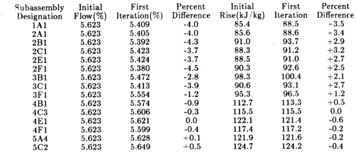
first is that the Newton-Raphson procedure is not necessary to obtain an estimate of the interassembly temperature profile. Table 1 shows the ratios of temperature rise to bulk temperature rise as well as the percent flow through each subassembly before and after the first Newton-Raphson iteration for a total flow of 5.6 % at 5.0% of full power. At this point the solution has nearly converged; about 30 out of 91 dimensionless pressure drop differences are outside the tolerance of 10-5. It can be seen that the adjustments to both the flow levels and the enthalpy rise are very small from one iteration to the next. Note that the percent change in enthalpy rise is even smaller than the percent change in flow level, as the transverse conduction tends to dampen the effect of the inlet flow on the outlet temperature.

A second important conclusion that can be drawn from this calculation is that the

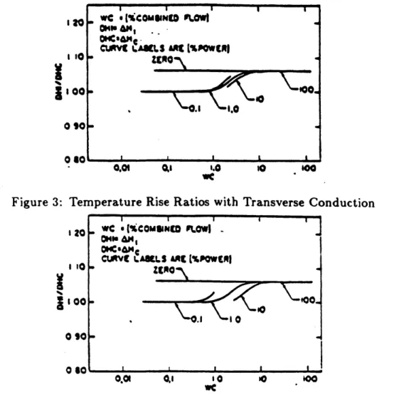
temperature rise ratios are only weakly dependent on power level. Table 2 shows the ratios of subassembly temperature rise to bulk temperature rise for power levels of 1.0, 3.0 and 5.0 % of full power (that is, for power levels characteristic of decay heat conditions.) Repeating this procedure for several flow/power combinations results in a series of tables whose graphical form is shown in Figure 3. These results can be compared to a similar set of tables illustrated in Figure 4. The Figure 4 results are obtained assuming no transverse conduction

[5].

The conduction effects explain the relatively weak dependence on power

level shown in Figure 3.

The characteristic shape of both sets of curves is most easily explained by referring to Figure 4. At 100% of full flow, the temperature rise across the channel is greater than the average-temperature rise; this is a "hot" channel. As the percent total flow decreases, the elevation pressure drop becomes dominant, and the flow within the hot channel increases. The inter-assembly profile flattens as the temperature rise across the

Subassembly Designation 1A1 2A1 2B1 2C1 2E1 2F1 3B1 3C1 3F1 4B1 4C3 4E1 4F1 5A4 5C2

Initial

Flow(%)

5.623 5.623 5.623 5.623 5.623 5.623 5.623 5.623 5.623 5.623 5.623 5.623 5.623 5.623 5.623 First

Iteration(%)

5.409 5.405 5.392 5.423 5.424 5.380 5.472 5.413 5.554 5.574 5.606 5.621 5.599 5.628 5.649 Percent Difference -4.0 -4.0 -4.3 -3.7 -3.7 -4.5 -2.8 -3.9 -1.2 -0.9 -0.3 0.0 -0.4 +0.1

Table 1: Variations in Dimensionless Flow and at 5.6 % of Total Flow and

Initial Rise(kJ /kg) 85.4 85.6 91.0 88.3 88.5 90.3 98.3 90.6 95.3 112.7 115.5 122.1 117.4 121.9 124.7 Enthalpy Rise 5.0 % Power First Iteration 88.5 88.6 93.7 91.2 91.0 92.6 100.4 93.1 96.5 113.3 115.5 121.4 117.2 121.6 124.2 Percent Difference -3.5 +3.4 +2.9 +3.2 +2.7 +2.5 +2.1 +2.7 +1.2 +0.5 0.0 -0.6 -0.2 -0.2 -0.4 Between Iterations Subassembly Designation 1A1 2A1 2B1 2C1 2E1 2F1 3B1 3C1 3F1 4B1 4C3 4E1 4F1 5A4 5C2 5.0 % Power 0.7597 0.7604 0.8042 0.7829 0.7818 0.7952 0.8623 0.7998 0.8287 0.9730 0.9918 1.042 1.006 1.044 1.067 3.0% Power 0.7499 0.7509 0.7957 0.7735 0.7736 0.7877 0.8556 0.7915 0.8247 0.9710 0.9915 1.044 1.007 1.045 1.068 1.0% Power 0.7391 0.7404 0.7863 0.7632 0.7646 0.7795 0.8483 0.7824 0.8205 0.9689 0.9914 1.047 1.008 1.046 1.070

Table 2: Variations in Ratio of Subassembly Temperature Rise to Bulk Temperature Rise Between Power Levels at 5.6

%

of Full Flow

20

I l0 ZERO\

1000.

Figure 3: Temperature Rise Ratios with Transverse Conduction

120 6 (*4cOMMUgD ULOWI --

T-CURVC LASILS ARC E%PfttMI

,10 t0 to.o..cusno I '0

zuo

S10 -0

90-0601

0.01 0,l 10 0 0 WC

Figure 4: Temperature Rise Ratios without Transverse Conduction

further, the elevation pressure drop becomes orders of magnitude larger than the friction

pressure drop, and the temperature rise across all channels is the same.

The strong dependence on power level illustrated in Fig. 4, the case without transverse

conduction, can be explained by considering the effect of power level on elevation pressure

drop. Since the.elevation pressure drop is dependent on the axial density profile, significant

differences in elevation pressure drops between channels do not occur until the temperature

rise across channels is significant. For low power levels, this does not occur until the percent

total flow is very low. Thus, the curves shift to the left with decreasing power level.

partic-ular channel is dependent on the axial temperature distributions in adjacent subassemblies as well as the flowrate within the subassembly. The temperature rise in a particular sub-assembly can change relative to the temperature rise in other subassemblies independent of the flowrate through that subassembly. Considering a low power, high total flow case, the amount of transverse conduction between subassemblies has a small absolute value, but it is comparable to the bulk temperature rise across the reactor. Thus, some flattening of the inter-assembly temperature profile takes place before the elevation pressure drop becomes dominant. The result is that the low power curves are pushed into the higher power curves, and the relative temperature rise across various parts of the reactor becomes a weak function of total power.

Using the results of this iterative calculation, we use a much simpler, faster procedure to obtain the temperature rise ratios as a function of flow only:

(a) Assume a power level in the reactor characteristic of decay heat conditions (i.e. 1 % of full power)

(b) Let the percent flow through each subassembly be the same as the percent total flow.

(c) Solve the coupled set of energy equations (4) to get the axial temperature profiles within each subassembly.

(d) Store these temperature rise ratos in a table as a function of flow.

3. Transient Heat Balance Models

A second way of using thermocouples to predict total flow through the reactor is

through a transient heat balance model (THBM). This can be accomplished if the decay power level in the reactor is known and an estimate of the bulk temperature rise across the reactor can be obtained.

3.1 Expressions for the Decay Heat

using a form of the ANS Revised Standard

[6].

The standard describes a variety of methods for estimating the decay heat in the reactor for any arbitrary operating history based on

23 different decay groups for each of three isotopes: U-235, U-238 and Pu-239. The form

of the decay power from a specific isotope for operation at a fixed level is:

23

F(t, T)

=

e~tt(1

-

e-AT)

(7)

Ai

i=1

where F(t, T) is the decay heat in MeV/fission, ai and Ai are decay constants, t is the time after shutdown and T is the length of operation at a fixed level. For some arbitrary operating history, the standard recommends that the decay power be calculated from:

3 M 23

P

Rj e "(1-e-A T,)

(8)

j=1 n=1 T=1

where P is the decay power in MeV/s, Rj, is the fission rate of nuclide

j

during operating

period T, (fissions/sec), T, is the operating period of length n seconds and t, -- t+

Z>

₁1 Ti

is the time after operating period n ended.

This algorithm gives the decay power as a function of time after shutdown, but it is in a computationally inefficient form. The problem is that the operating history must first be tabulated, then broken into discrete operating levels before the algorithm can actually be used. Tabulating the operating history may require large amounts of storage space, and some normal operations, such as a ramp up to full power, may not be easily represented

by a set of discrete operating levels. An alternative approach is to continuously update

the contributions from each of the 23 decay groups while the reactor is running. This eliminates the problem of partitioning the operating history. Let Xi be the normalized

contribution from decay group i where gis the normalization constant for group i; let

N be the normalized neutron power where P is the normalization constant. Then the

contribution from decay group i may be updated using:

dX,

= Aj(N - Xj)

(9)

During operation, the contribution from each Xi is calculated from

(Xi),ew = (XI)old + Aizt(N - (Xi)old) (10)

When the reactor shuts down, the initial contribution from each decay group is:

Xio = (Xi)s own (11)

and the decay power is calculated from:

P = Rj Xioe- (12)

i=1

3.2 Stored Energy Removal

In addition to the decay heat, there is a certain amount of energy removed from the mass of the reactor during the early part of the transient. This stored energy removal, Se, has the form:

Se

=

c

pMi

(13)

where Se is the stored energy removed, OT is the change in bulk sodium and reactor material temperature per unit time, c, is the specific heat of the ith material and Mi is the mass of the ith material. This term is then added to the decay heat term in the transient heat balance equation.

3.3 Transient Heat Balance Equation

The decay power and the stored energy removal are used as inputs to the transient heat balance equation, which is used to predict the flow through the reactor. The heat balance equation is:

pVc,

at

+ MTCPATc

Q

+ Se (14)

The quantities 4T1 and ATc can be ascertained from temperature measurements, and the

_{a t}

decay heat and stored energy removal are calculated as stated above. The equation can then be solved for the mass flowrate MT.

4. Signal Validation Techniques

Whenever possible, the inputs to both AHBM and THBM models are validated prior

to use in the model. In AHBM, the subassembly outlet thermocouples are used without any modification. The reactor inlet temperature, which was validated for use in comparisons of direct and analytic flows in Test 8A

[3),

was not validated in this model because only one reactor inlet thermocouple (HPPTCT) was monitored by the Data Acquisition System.

Two analytic measurements of flow are obtained with the THBM by using two dif-ferent sets of thermocouples to obtain independent validated outlet temperatures for use in the model. In THBMS, a validated outlet temperature is obtained using two levels of decision/estimators (D/E's). The details of the algorithm used in the D/E's are discussed in [3]. Basically, the validated outlet temperature is a weighted average of the input tem-peratures, where the weighting is established from the inverse standard deviations of the inputs. In the first level, validated outlet temperatures are obtained for rows 1 and 2 (output VHP1 is obtained from subassembly outlet thermocouple (SOT's) 1A1, 2A1, 2B1,

2C1, 2E1 and 2F1), for row 3 (output VHP3 is obtained from SOT's 3B1, 3C1 and 3F1),

for rows 4 and 5 (output VHP4 obtained from SOT's 4B1, 4C3, 4E1, 4F1 and 5A4), for rows 5,6 and 7 (output VHP5 obtained from SOT's 5C2, 6C4, 7A3 and 7D4) and for the low pressure plenum outlet (VLPP from SOT's 9E4, 12E6 and 16E9). In the second level, a validated subassembly reactor outlet temperature (VSROT) is obtained from VHPI, VHP3, VHP4, VHP5 and VLPP. The inlet temperature is again not validated because only one reading exists.

In the second calculation (THBMO), the validated outlet temperature is obtained using a single D/E which delivers a validated reactor outlet temperature (VROT) from thermocouples ROTCCF, UPTC1, UPTC2 and UPTC3. It is important to note the differences between the location of these thermocouples and the subassembly outlet ther-mocouples used in THBMS. Thermocouple ROTCCF is located on the outlet Z-pipe of

EBR-II, just after the fluid leaves the reactor vessel. Thermocouples UPTC1, UPTC2 and

UPTC3 are mounted on a finger suspended above the fourteenth row of the reactor. Thus

the two sets of thermocouples used in THBMO and THBMS sample two different regions of the reactor. As with THBMS and AHBM, the inlet temperature of THBMO is not validated.

For the direct measurement, two magnetic flowmeters (MFHPP2, MFLPP2) were used. The two flowmeters measure flow to the high pressure and low pressure plenums on leg 2 respectively. Before validation, each flowmeter was properly calibrated. To establish the proper calibration parameters, a linear regression was performed with expected true values and raw measured values. The expected values were calculated using the weighting factor of each flowmeter based on their inverse standard deviations. In the estimate routine for the direct measurement, the weighting of the flowmeters was not based on the inverse standard deviation but was based on the flowrate ratio through the respective inlets. These weights were chosen to reflect the relative contributions of the inlet plenums to the total

flow, not because one reading was more accurate than another. The high pressure plenum

weighting was thus considerably higher than that of the low pressure plenum.

5. Testing the Methods.

To determine the validity of these analytic techniques, a data tape from the Shutdown Heat Removal Tests (SHRT) was obtained for tests 2, 3, 4, 11 and 12. These five tests were chosen for comparison because they represent a range of different initial reactor test conditions. The-individual analytic measurements were compared with the direct flow measurements, and a validated flow estimate was obtained from the individual analytic measurements and the direct flow measurement.

To obtain the final validated flow estimate, the weighting scheme for the direct mea-surement and the three analytic meamea-surements usually consists of a constant weighting

for the direct measurement and an inverse standard deviation weighting for the analytic measurements. The constant weighting for the direct measurement has been taken as 1/3. For this particular set of tests, the weighting for each of the remaining three analytic mea-surements has been taken as 1/3 of the remaining 2/3; that is, each analytic measurement was weighted by 2/9.

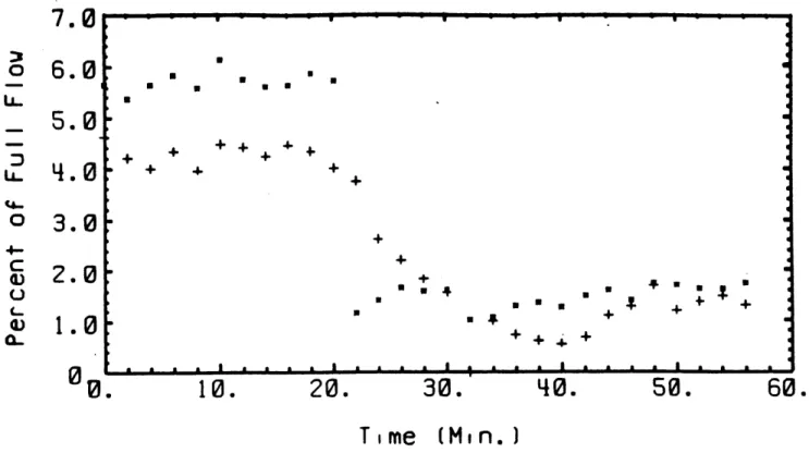
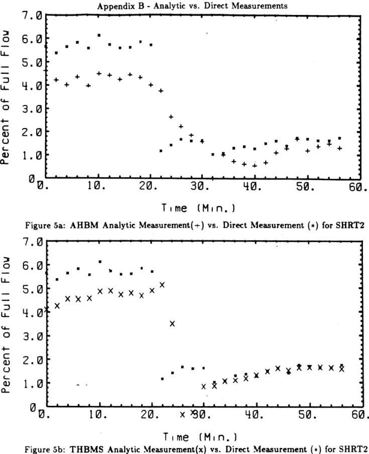
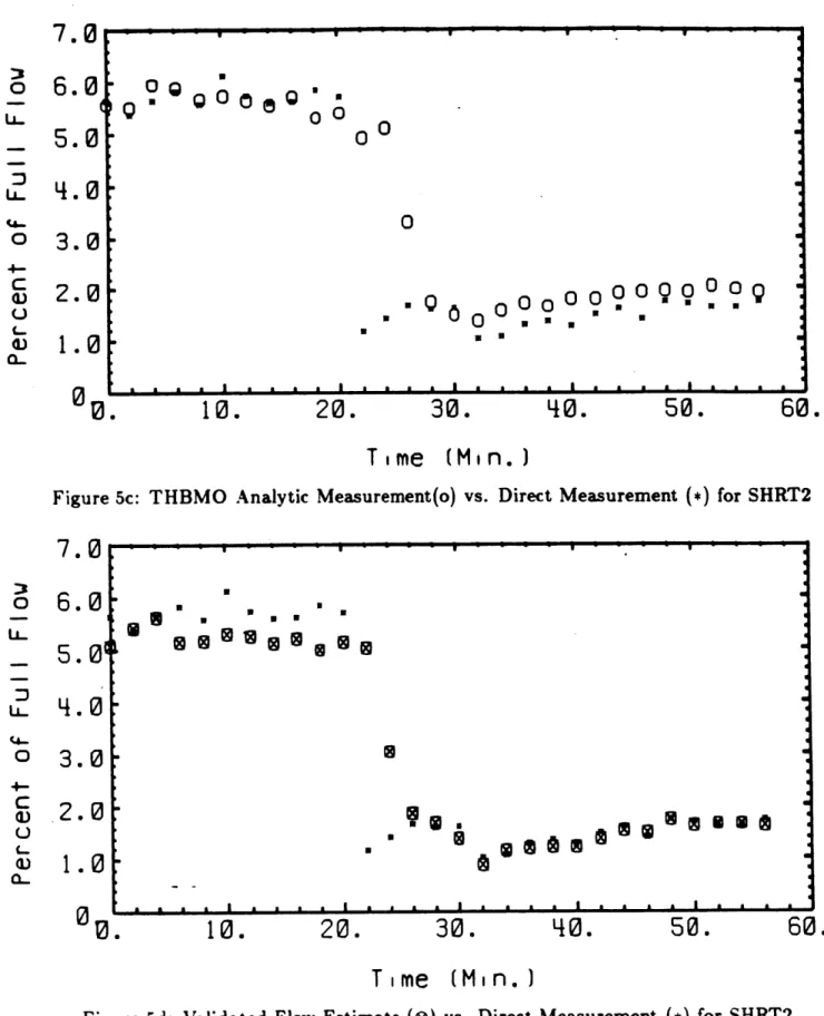
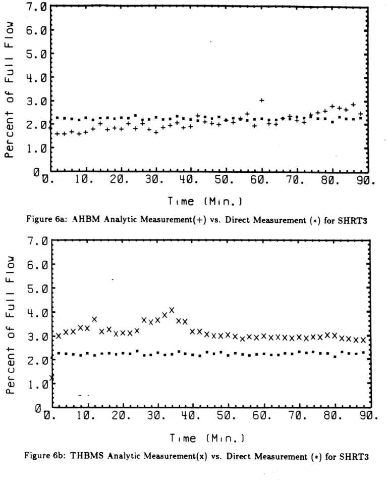
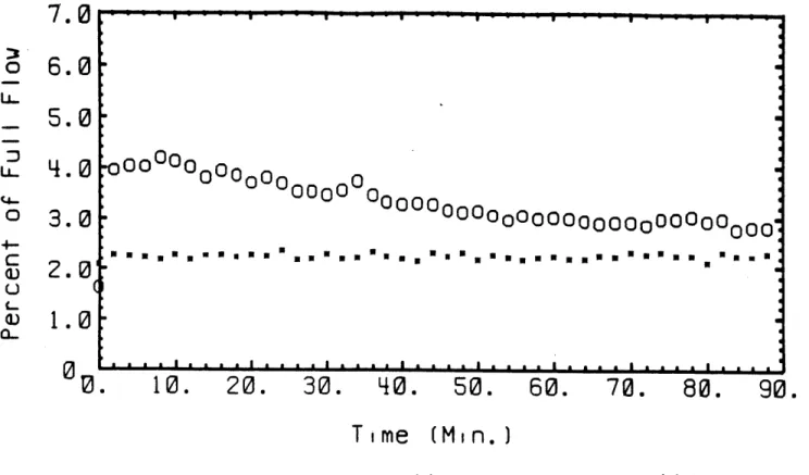
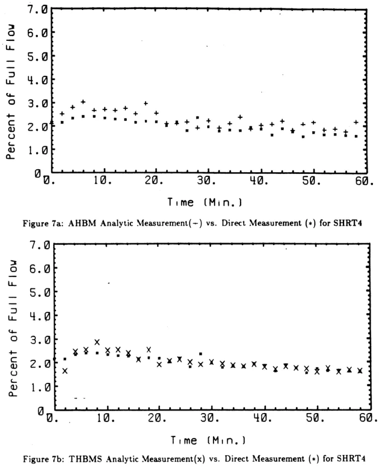
Figures 5a and 5b compare the AHBM and THBMS analytic measurements with the direct flow measurement in SHRT2 respectively. A copy of these plots, as well as Figures 5c (THBMO vs. direct flow) and 5d (validated vs. direct flow) and the corresponding plots for SHRT3 (6a-d), SHRT4 (7a-d), SHRT11 (8a-d) and SHRT12 (9a-d) appear in Appendix B. Agreement between the individual analytic and direct measurements is generally good, although there are some exceptions. Despite these differences, the validated flow estimate is consistently close to the measured flow. Taking SHRT3 as an example, it can be seen that the validated flow estimate remains remarkably close to the measured flow, despite the fact that THBMO and THBMS consistently overpredicted the flow.

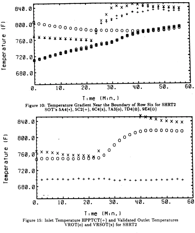
There are several sources of error which contribute to the observed discrepancy. The first type of error can be described as model-related error. One of the assumptions made in AHBM is that the first six rows are isolated from the rest of the reactor; that is, the boundary between rows six and seven is insulated. This is a reasonable assumption only if the temperature gradient around this boundary is relatively flat. Figure 10 plots the subassembly outlet temperatures 5A4, 5C2, 6C4, 7D4, 7A3 and 9E4 for SHRT2; this plot, as well as those for SHRT's 3 (Figure 11), 4 (Figure 12), 11 (Figure 13) and 12 (Figure 14) are listed in Appendix C. These results indicate the temperature gradient is not always flat; in some instances, as in SHRT2, SHRT3 and in the low flow portion of SHRT12, the heat flow tends to be outward from the inner six rows to the outer ten rows. Including this effect in the model would tend to further flatten the temperature rise ratios, which would result in higher and better predictions of flow.

30.

Time

(Min.)

AHBM Analytic Measurement(+)

10.

20.

vs. Direct

x

90.

Measurement (*) for SHRT2

40.

50.

60.

Time

(Min.)

Figure 5b: THBMS Analytic Measurement(x) vs. Direct Measurement (*) for SHRT2

7

0 LL '4-0 C (U

a-5.0

2.0

1.0

0

+ 4- + + 4L + 4-+

10.

20.

Figure 5a:

40.

7.0

50.

60.

DI

0 LL U-0 4-C CU U C-CU

a-5.0

4

3.0

2.0

x

xxX xx x x x x

-x - X x x Sx x

.

0

.

0

_.

In addition, it is assumed in the solution procedure that the percent power within each subassembly is the same as the percent power within the reactor. This assumption is not always correct; some of the subassemblies within the core contain little or no fuel and generate no decay heat. The degree to which these subassemblies act as a heat sink therefore tends to be greater than that described by the model.

A second type of error that is responsible for the observed discrepancy between

pre-diction and experiment is sensor-related error. For these validation tests, only one input was available for the reactor inlet temperature and for the direct flow. Errors in the for-mer of these measurements would be strongly felt in the analytic models. In SHRT12, for instance, the initial reactor tank temperature was supposedly 680 F; the other SHRT tests all had inlet temperatures of approximately 700 F. However, Figure 19 in Appendix

D clearly shows an inlet temperature reading of approximately 700 F. For a nominal rise

of 100'F, this would tend to result in a predicted flow 20 % too high.

Finally, the position of the sensors in the reactor can contribute to the error in the analytic models. In SHRT tests 3 and 12, where THBMS and THBMO perform poorly, it can be seen that THBMO tends to perform more poorly than THBMS. This can be attributed to the location of the input sensors for THBMO. The three upper plenum ther-mocouples used in THBMO are located in a part of the upper plenum which tends to be relatively cool. The reactor outlet thermocouple, located on the outlet Z-pipe, measures the flow temperature after the flow has had an opportunity to transfer heat to the bulk pool which surrounds the reactor vessel. This implies the validated reactor outlet temper-ature (VROT)-will tend to be lower than the validated subassembly outlet tempertemper-ature (VSROT). Figure 15 shows the inlet thermocouple reading (HPPTCT), VROT and

VR-SOT for SHRT2; this figure, as well as those for SHRT3 (Figure 16), SHRT4 (Figure 17),

SHRT11 (Figure 18) and SHRT12 (Figure 19) also appear in Appendix D. The plots tend to support the preceeding explanations.

840.0

800.0

760.0

720.0

680.e

0.

10.

20.

30.

40.

50.

Time (Min.)

Figure 10: Temperature Gradient Near the Boundary of Row Six for SHRT2

SOT's 5A4(*), 5C2(+), 6C4(x), 7A3(o), 7D4(@),

9E4(e)

840.

800.

760.0

720.

680.

0.

10.

20.

30.

q0.

50.

T

me (M

in. )

Figure 15: Inlet Temperature HPPTCT(+) and Validated Outlet Temperatures

VROT(o) and VRSOT(x) for SHRT2

4-(U 3. E 0) 0) L.. 4-(0 C... ~1) 0. 2

a)

60.

60.

6. Summary and Conclusions

Two models have been presented which provide analytic measurements of

the

total

flowrate in the EBR-II reactor during natural circulation. The first model presented was

the Assembly Heat Balance Model (AHBM). This model predicted the total flow through

the reactor on the basis of tabulated ratios of temperature rise across one subassembly

to the temperature rise across another subassembly. Because so many subassembly outlet

thermocouples exist in the EBR-II reactor, this model is inherently redundant.

Previous work related to this model

[5]

indicated that these ratios would be functions

of both total flowrate and total power level in the reactor; however, after solving the

problem for multiple power levels as described in the beginning of Section 2.4 for the

specific case of EBR-II the dependence on power level was found to be extremely weak.

In addition, the iterative solution suggested a simpler, much faster solution procedure.

Both effects are attributed to the excellent transverse conduction between subassemblies

at natural circulation flows. A comparison of the flowrates predicted by this model with the

direct flow measurements from the SHRT tests indicated that the model is basically sound;

however, room for improvement exists with respect to the applied boundary conditions.

A second nodel was presented called the Transient Heat Balance Model (THBM).

This model used the decay heat in the reactor and the time-dependent behavior of two

different validated reactor outlet temperatures to infer the flowrate. Comparison of the

flowrates predicted by model THBMS (based on validated reactor outlet temperature

from subassembly outlet thermocouples) and THBMO (based on validated reactor outlet

temperature from upper plenum probe and reactor outlet thermocouples) indicated that

these models are also sound except when the temperature rise across the reactor is very

small. In those cases, the predicted flow can vary greatly from the measured flow. THBMO

is particularly prone to error as its group of outlet thermocouples tend to read lower than

those of THBMS.

Despite the occasional poor predictions, the validated flow estimate obtained from the individual analytic measurements and the direct flow measurment was consistently in good agreement with the measured flow. The validation architecture performs admirably even when some of its inputs are errant.

Appendix A - Newton/Raphson Method

The exact form of the Newton-Raphson procedure used in the solution procedure is described here. First, define a normalized pressure drop difference:

Ap - AP

S1,

2, ..., 91

(A1)

where

Api = pressure drop across ith subassembly calculated from (1) in step (d) of the solution procedure,

Ap'= actual pressure drop acros the reactor (unknown), initially set equal to

APa,

Apa = approximate pressure drop across the reactor calculated in step (b) of the

solution procedure.

Also define a normalized mass flowrate difference:

/ -MT -(2

92 = (A2)

These quantities are functions of the normalized mass flowrates and pressure drop, defined as:

z=

;i =

1,2,...,91 (A3)

mi,full

where

mt = mass flowrate in ith subassembly

mi,full -= mass flowrate in the ith subassembly during full flow.

X92 =

(A4)

Considering Y and Y as vectors,

where

o= initial guesses of normalized mass flowrates,

'o

=

(zo)

= results from initial guesses of i,

S1 = next set of guesses of normalized mass flowrates,

= ₁(51) = results from next set of guesses of 5,

a

= Jacobian of V with respect to i.

A next set of mass flowrates can be found by first solving for the Jacobian. This can

be done by perturbing the flow in one subassembly, executing steps (a)-(d) in the solution procedure, and repeating the calculation for all subassemblies. Solving for the value of -1 that will yield 01 = 0 gives the next set of guesses for the flowrates:

Appendix Notes For Appendices B,C and D:

(a) For the plots appearing in Appendices B,C and D, the time t = 0 does not correspond to time t = 0 on the DAS system. This is due to the fact that the flow and power at the beginning of the tests were appreciably larger than flow and power characteristic of natural circulation. These portions of the tests have not been shown. For SHRT2, time t = 0 corresponds to a DAS time of 2392 s into the test. For SHRT3, SHRT4 and SHRT1I time t = 0 corresponds to 1432 (DAS) into the test. For SHRT12, time

t = 0 corresponds to 1672 (DAS) into the test.

(b) In Figures 6b and 9b, there appear substantial fluctuations in the flow predicted by

THBMS. The source of these fluctuations lies in smaller fluctuations found in the Validated Subassembly Reactor Outlet Temperature (VSROT); the time derivative terms in the transient heat balance equations are amplified by this low level, high frequency noise. The source of the noise in VSROT is itself unknown.

(c) In Figure 15 in Appendix D, the VSROT is off-scale high during the first part of the transient after the auxiliary pump is shut off. This is why there is no validated VRSOT (x) shown in a portion of this plot.

(d) In SHRT's 2 and 12, there is a rapid change in flow caused by the shutdown (SHRT

Appendix B

-

Analytic vs. Direct Measurements

10.

20.

30.

40.

50.

60.

Time (Min.

)

Figure 5a: AHBM Analytic Measurement(-t-) vs. Direct Measurement (*) for SHRT2

10.

20.

x

)0.

T

i me (M

in.)

40.

60.

Figure 5b: THBMS Analytic Measurement(x) vs. Direct Measurement (*) for SHRT2

7.0

6.0

5.0

4.0

3.0

2.0

1.0

o 0 U-IL f4-0 C 0

a-0

7.0

6.0

5.0

4. 0,

0 o '4-0 4. C U

3

2

0

0

. x x

x

- X X X -a J- -- a aa a Jp M a a a a -M a a

1.0

0.

.

.

50.

00 0 5 0 IQ

00

:1 0 U- LL-0 C (A) 0-U

99??Q

- " - - - - I

-10.

20.

30.

0

.

410.

090

"

-60.

T

ime

(M

in.

)

Figure 5c: THBMO Analytic Measurement(o) vs. Direct Measurement (*) for SHRT2

10.

20.

30.

410.

60.

T ime

(Min.)

Figure 5d: Validated

Flow

Estimate

(9)

vs. Direct Measurement (*) for SHRT2

0

5.0

q.

0

3.0

2.0

1.0

0

.

7.0

6

D3 0 o LL- .4-0

C

0

0-3

0|

U UU

U,

* U

e

U

U -- 4 * AM A I * I * I * * I * A I A A A

2.0

1.0

00

I w w 4

a

. . . . a . . . . a . . . 2 a

50.

0

f

.

5.0

4.0

.

.a

50.@

0 4-C U.) U- L-(U)

0-a n 0n a In nU + + + + ++

~

U. * ₊ * ~ -. +4. +

10.

20.

30.

40.

50.

60.

70.

80.

90.

Time (Min.)

Figure 6a: AHBM Analytic Measurement(+) vs. Direct Measurement (*)

7.0

for SHRT3

6

5.0

-3.0

2.0

1.0

x XxXXXXX U XXx xx XXXxxxxxxxxxxxxxxxxxxx

.X

xx. -n

a

0

n UR

.

10.

20.

30.

40.

50.

60.

70.

80.

90.

Time

(Min.)

Figure 6b: THBMS Analytic Measurement(x) vs. Direct Measurement (*) for SHRT3

7.0

6.0

5.0

4.0

3

2.0.

1.0

+

*

::

+ U I.... U - - - U :3 0

U-o

a> 0 4-C w3 U-I

-.a

a S

S a I

a S

a a

I

S a

. a I . . . . I . . . . I . .

.

.

.

-.

-. I . . . . I . . . . I . . . . a . . . . a . . . . I . . . . I . . . . a . . . .I

7.0

6.0

5.0

4.0

3.0

2.0'

1.0

THBMO Analytic Measurement(o) vs. Direct Measurement (*) for SHRT3

6

5.0-4.0

3.0

1.0

0

some

.. uUN.U...N.NUUEE *g~U~

:000

I a a a. a I a 1 I. a I

10.

20.

30.

40.

50.

60.

70.

80.

90.

Time

(Min.)

Figure 6d: Validated Flow Estimate (0) vs. Direct Measurement (*) for SHRT3

:o 0 U- 4-C oU C-CU) c0

-

000000

000,00

0

0000 000

-oo000000oooooooooooooo

10.

20.

30.

40.

50.

60.

70.

80.

90.

Time (Min.)

Figure 6c:

7.0

D3 0 U-u_ 0 4... C

a-)

0U - V - - - - - - - - - - - - - - - - - - - - - - - - -i - - . . a a a a a a S a a a 2 0 a a a

I

a

.

-I U

7.0

6.0

5.0

4.0

3.0

2.0

1.0

o

U_

U_

0 IL IL0 4-C (U a-. + .4+ +++ ₊ * ₊ n + + t+. .+ . . -, -, 4 4 . . . t+ a - a - .

40.

50.

Time (Min.)

Figure 7a: AHBM Analytic Measurement(-)

vs. Direct Measurement (*) for SHRT4

7.0

6.0

5.0

1.0

3.0

2.0

1.0

I I I

x

V

x

I

2 a 1 a a 2 2 - I I I

10.

X

-I

X

x x

4x

20.

30.

40.

50.

T

ime (Min.)

Figure 7b: THBMS Analytic Measurement(x) vs. Direct Measurement (*) for SHRT4

+ +-LU - a

10.

20.

30.

60.

o 0 U_

o

0 C 0a. U.

60.

a I I I I

I

10.

20.

30.

40.

50.

60.

Time (Min.

)

Figure 7c: THBMO Analytic Measurement(o) vs. Direct Measurement (*)

7

_.0

L-6.0

S.0[

4.0

3.0

2.0t

1.0

0

_0'.

10.

20.

30.

40.

50.

for SHRT4

60.

T i

me (M

in.

)

Figure 7d: Validated Flow Estimate

(0)

vs. Direct Measurement (*) for SHRT4

7.0

6.0

5.0

3.0

2.o

1.0

=9 0 LL LL o 0 0) U 0-Dt 0 -IL (4-0 C U o-

Q Q 9 e 8

.aa@

8eses

Cg

_e

I . . . . I . . . I . a I I a a a a I a * i i

-U :: 0 LL IL_ 0 C- 0-* U - * * U 4- ++ - -U + U * * R U * + + ++ ++ 4- ++ + + I . . . . a

20.

a - - - - a

30.

40.

T

ime

(M

in. )

Figure 8a: AHBM Analytic Measurement(+) vs. Direct Measurement

7.0

6

5

3

2

1

(*) for SHRT11

x _-x _x X x x _X4 X x

0

01

0

0

F

U

X

xxx

-x

x

4 4 a

10.

20.

- - 4 - - - a - - - - a

-30.

40.

50.

60.

Time

(Min.)

Figure 8b: THBMS Analytic Measurement(x) vs. Direct Measurement (*) for SHRT11

7.0

N

5.0

4.0

3.0'

2.0

1.0

0 * UL +

10.

_50.

_60.

:3 0 LL IL 4-C CU U NdNEW.w4W.mog - - - S a a -- a - a a A a 0

LmwnLo-A--A-a LmwnLo-A--A-a -LmwnLo-A--A-a-- LmwnLo-A--A-a

a

2 S a 2

S

- S a

Ik a

S

I S N a 0

.

.

-4. 0

.

.

.

10.

20.

:o 0 u 0 4-C

Q-40.

60.

THBMO Analytic Measurement(o) vs. Direct Measurement (*) for SHRT11

10.

20.

30.

40.

50.

60.

Time (Min.

)

Figure 8d: Validated Flow Estimate (0) vs. Direct Measurement (*) for SHRT11

7.0

6.0

91.0

3.0

2.0

1.0

0 .

_30.

Time (Min.)

-a

o o

Q 4

0

"

a a a a

a a a a

Figure 8c

7.01

o IL L 0

a-6.0

5.0

4.0

3.0

2.0

1.0

-a

- a

A-50.*

:

I

.

0

7.0

6.0

5.0

41.0

U-0 .4-C CU. CU a_)

2.01

1.1

0 0

_20.

_40.

_60.

_80.

_100.

_120.

Time (Min.)

Figure 9a: AHBM Analytic Measurement(+) vs. Direct Measurement (*) for SHRT12

x

7.0

20.

40.

60.

80.

100.

N

x)'XxxxXxxxx~x

. " "

x x

x

x

x XX XX x _xxx "" "m".-a _a ""m"ana"-"X _N "

X'X""

_N * *x * N* BIB

120.

Time

(Min.,)

Figure 9b: THBMS Analytic Measurement(x) vs. Direct Measurement (*) for SHRT12

3

+ * ++n + + a o 0 o as Sam s *a now*ONE -- +4++++++4.4.+++++.H. + +.f++ +.+ ++ + ++ 4+ .+. + +

6

5

4.0

3.0

2.01

D9 0 oL U-0 i. U Q-

₁

.0

0

a a a I a aa

a~~~~

a I a a a a I

a

a. a II

_~~~

a B B I a a _a

.

.a

-

-

-I

-x -x.

--..

x-o-.

.

x .s

60.

80.

Time (Min.)

Figure 9c: THBMO Analytic Measurement(o) vs. Direct Measurement (*)

7.0

6.0

5.0

4. 0

3.0

2.0

1.0

for SHRT12

20.

40.

60.

80.

100.

120.

Time

(Min.)

Figure 9d: Validated Flow Estimate

(0)

vs. Direct Measurement (*) for SHRT12

0

0

7.0

6.0

5.0

3.0

2.0

1.01

DR

0

IL 0 (-0.)

0-00

0

0

..

30

wo

EpNN

o

onNo

MN on

asa@onP0NMMM

001

20.

40.

100.

120.

:3

0

IL a> 0

C

U

S S a

.

0

O.

Appendix C

-

Temperature Gradients Near the Boundary of Row Six

x xx x- _{. +}

X +x+

760.0

720.

x

s t

0

o

₊ 0 _{000 000}

a

680.0 [

00

₀

_6gg

a

w

gges

10.

20.

30.

40.

Time (Min.)

Figure 10: Temperature Gradient Near the Boundary of Row Six for SHRT2

SOT's 5A4(*), 5C2(+), 6C4(x), 7A3(o), 7D4(&),

9E4(e)

840.0

800.0

760.0(

720.01

680.0

0.

10.

20.

30.

40.

50.

60.

70.

80.

90.

Figure 11: Temperature

SOT's 5A4(*),

Time

(Min.)

Gradient Near the Boundary of Row Six for SHRT3

5C2(+), 6C4(x), 7A3(o), 7D4(g),

9E4(e)

840.0

800

(0

E a~)

aU88

50.

60.

U-a.)

(0

a.)

000

0

0

- --- -- - -- - - i - - - - - a .. 46 ... IV ... "

-.

a

01

4 2

0.

8'40.0

800.0(

760.0

720.0

0000o

0000

₀₀₀₀

x

6

eil

68666l,

a

.

.

a .

.

a

10.

20.

30.

40.

50.

60.

Time (Min.)

Figure 12: Temperature

SOT's 5A4(*),

x

840.

800.0

760.0

720.0

680.0

0.

10.

Gradient Near the Boundary of Row Six for SHRT4

5C2(+), 6C4(x), 7A3(o), 7D4(®),

9E4(e)

20.

30.

40.

50.

T i

me (M

in.

)

Figure 13: Temperature Gradient Near the Boundary of Row Six for SHRT11

SOT's 5A4(*), 5C2(+), 6C4(x), 7A3(o), 7D4(0),

9E4(e)

6

CU (0 C

6 8 0

_.

0

_r

0.

L 4-(0

C-a)

0l

E

a)

e 0 00 0

00

0 0 0 0

o

0 00o00o0oo 0u0 000u00

g g

60.

8

_{E3 6}

@@IN 14

a

I

I

10

840.0

I-

800.0

600**x

+

++

720.0

Eo89

680.0

0.

20.

40.

60.

80.

100.

120.

Time (Min.)

Figure 14: Temperature Gradient Near the Boundary of Row Six for SHRT12

SOT's 5A4(*), 5C2(+), 6C4(x), 7A3(o). 7D4(®),

9E4(e)

840. 0

800.0

760.0

720.0

680.0

10.

20.

30.

40.

50.

60.

Figure 15:

840.0

800.0

04

720.0

680.0

0.

T i

me (M

in. )

Inlet Temperature HPPTCT(+) and Validated Outlet

VROT(o) and VRSOT(x) for SHRT2

20.

40.

60.

Temperatures

80.

Time (Min.)

Figure 16: Inlet Temperature HPPTCT(+) and Validated Outlet Temperatures

VROT(o) and VRSOT(x) for SHRT3

C.

4-E

c-E

Appendix D

-

Inlet and Validated Outlet Temperatures

w

X x x x x

oooooooooo

- 0

0

0

X X X X X x x x X 0

o o

0 0 0 0 0

o

ox

6

60o

+O

OOO~~

0

++

+++++4

a a M a a a a a - -a a- a M S a 3k a M a a p LL-(U) L-CIL

E-aU

760.

a I I U

:xxxxxxxxxx

LOoooooooooo~9~e~e~,se..

+ I S I p I p p I P I P I * *

0.

840.0

800.0

760.0

720.0

680.0

0

10.

20.

30.

40.

T i

me (M

in.

)

Figure 17: Inlet Temperature HPPTCT(+) and Validated Outlet

VROT(o) and VRSOT(x) for SHRT4

840.0(

800.0

760.0

720.0

680.0

0.

10.

20.

30.

40.

60.

Temperatures

50.

60.

Time (Min.)

Figure 18: Inlet Temperature HPPTCT(+) and Validated Outlet Temperatures

VROT(o) and VRSOT(x) for SHRT11

0-% 4L-

C-a

E 7

--9

00o

x 0

aA

0 o

a A

_{9 9 9}

9

X

X

_{X X}

X- 4-(o C-Ga) CIL

.6

+

-+ + + + + + + + + + +

.

50.

I