Design and analysis of double-layer grids

DESIGN AND ANALYSIS OF DOUBLE-LAYER GRIDS By

WANG-REI TANG

Bachelor of Science in Architecture and Architectural Engineering Technical University of Budapest

June 1998

Submitted to the Department of Civil and Environmental Engineering In Partial Fulfillment of the Requirements for the Degree of

MASTER OF ENGINEERING

IN CIVIL AND ENVIRONMENTAL ENGINEERING

At the

MASSACHUSETTS INSTITUTE OF TECHNOLOGY

June 1999

@1999 Wang-Rei Tang All rights reserved

The author hereby grants to M.I.T. permission to reproduce and distribute publicly paper and electronic copies of this thesis document in whole or in part.

Signature of the Author_

Certified by

Accepted by

Departmerf of Civil and Environmental Engineering May 7, 1999

J

' PBofessor Andrew J. Whittle Chairman, Department Committee on Graduate Studies

DESIGN AND ANALYSIS OF DOUBLE-LAYER GRIDS By

WANG-REI TANG

Submitted to the Department of Civil and Environmental Engineering on May 7, 1999 in partial fulfillment of the requirements for the degree of Master of Engineering in Civil

and Environmental Engineering

Abstract

This thesis focuses on the design and analysis of double-layer structural grids. The analysis is based on the use of formex algebra. Basically, formex algebra is a mathematical system designed to deal in a convenient way with problems of data preparation and graphics in computer aided design processes. Formex algebra is particularly useful for space structures having complex geometry. Following the formex formulation, one case study is considered. Two models of double-layer grids are

designed and analyzed using SAP and ADINA.

Thesis Supervisor: Title:

Jerome Connor

Acknowledgements

First of all, I would like to thank my advisor, Professor Jerome Connor, for all his help

during the entire year, for his understanding and trust in whatever I was doing. Thanks to

Charlie Helliwell for his support to the M.Eng. program in general, and to the HPS

project and thesis in particular. Thanks to the structure group for their contribution to our

group project. Thanks to all my classmates in the M.Eng group for all the happiness we

spend together.

Very special thanks to my parents, brother and for their continuous support for whatever

decision I made. Thanks to my relatives and friends for their support through all these

years.

TABLE OF CONTENTS

TA BLE O F FIG U R ES... 5

CH A PTER O N E BA C K G R O UN D ... 6

CHAPTER TWO FUNDAMENTALS OF FORMEX ALGEBRA...8

2.1 INTRODUCTION ... 8

2.2 SIGNETS... 8

2.3 CANTLES ... 10

2.4 FORM ICES... 12

2.5 COM POSITION OF FORM ICES ... 15

2.6 LIBRA NOTATION ... 16

CHAPTER THREE FORMEX PLOTS...18

3.1 INTRODUCTION ... 18

3.2 RETROBASES ... 18

CHAPTER FOUR FORMEX FUNCTIONS... 21

4.1 INTRODUCTION ... 21

4.2 TRANSLATION FUNCTIONS ... 23

4.3 REFLECTION FUNCTIONS... 27

CH A PTER FIV E CA SE STU D Y ... 29

CHAPTER SIX STATIC ANALYSES OF DOUBLE-LAYER GRIDS ... 35

6.1 G EOM ETRY ... 35

6.2 STRUCTURAL ANALYSIS ... 35

6.3 N UM ERICAL SOLUTION ... 36

CHAPTER SEVEN DESIGN OF A SPACE TRUSS ROOF ... 38

7.1 G EOM ETRY ... 38

7.2 STRUCTURAL ANALYSIS... 38

7.3 M ERO SYSTEM ... 39

CH A PTER EIG H T C O N CLU SIO N ... 42

A PPEN D IX A... 44

A PPEN D IX B... 50

A PPEN D IX C ... 68

TABLE OF FIGURES FIGURE 3.2.1 FIGURE 3.2.2 FIGURE 3.2.3 FIGURE 4.2.1 FIGURE 4.2.2 FIGURE 5.1 FIGURE 5.2 FIGURE 6.1 FIGURE 7.2.1 FIGURE 7.2.2 FIGURE 7.3.1 FIGURE 7.3.2

PLOT IN TWO-DIMENSIONAL CARTESIAN COORDINATE SYSTEM 1 PLOT IN TWO DIMENSIONAL CARTESIAN COORDINATE SYSTEM 2 PLOT IN POLAR COORDINATE SYSTEM

AN EXAMPLE OF FORMEX PLOT OF TRANSLATION FUNCTION 1 AN EXAMPLE OF FORMEX PLOT OF TRANSLATION FUNCTION 2

NORMAL Z-PLOT

OBLIQUE Z-PLOT

GRID GEOMETRY

PLAN VIEW OF THE STRUCTURE IN SAP ELEVATION VIEW IN SAP

A STANDARD MERO CONNECTOR

CHAPTER ONE

In the past, space structures were regarded as exotic and unconventional. Now, they are

used frequently in many countries around the world, not only because they are

aesthetically pleasing but also because they are efficient structural forms.

Over the last century, engineers have been striving to build larger and larger structures

with less material and less cost. Designers agree that for large spans, conventional beam

and truss structures prove to be uneconomical, and have turned to three-dimensional

structures which have incredible rigidity and the ability to cover large spans with

minimum weight.

Double-layer grids have developed rapidly in the past several decades. They are suited

for covering exhibition pavilions, swimming pools, and many types of industrial

buildings in which large unobstructed areas are required. Experience shows that in many

countries double-layer grid structures can compete very successfully with more

conventional systems. Due to the complex and regular nature of double layer structural

grids, it is convenience to use computer techniques for the design and production process.

One of the main problems in design is generating the data required for the phases of the

numerical model used in analysis models, and in general, dealing with large amounts of

data. The data required by a numerical model of a reasonably large structure is

substantial. The input includes the nodal coordinates, the connectivity, element

properties, boundary or support conditions and the applied loads. Formex algebra may be

used in various ways to overcome the difficulties of data preparation. In particular, the

description of the interconnection pattern of a structural system may be conveniently

CHAPTER TWO FUNDAMENTALS OF FORMEX ALGEBRA

2.1 Introduction

Formex algebra is a mathematical system that consists of a set of definitions for numerical objects, and a set of rules for manipulating these objects. Formex algebra is the basis of this paper and all the techniques that simplify the work of data preparation and graphics in computer aided design processes. Formex algebra allows all kinds of

networks to be formulated conveniently. In what follows, the basic definitions and rules

are introduced.

2.2 Signets

A 'signet' is an object of the form

[I1, 12, 13, 14,..., In]

where n is greater or equal to 1 and where I1, 12, 13, 14,..., In are integers. For example,

[3] [5, 2] [-4, -3, 9] and [45, 98, -3, 8, -45] are signets.

'4', '7', '11' and '1' are said to be the indices of the signet. Since there are four integers

in the signet, the signet is of the grade 4.

In order to have a relationship between two signets, such as 'equal', 'greater than' or 'less

than', the two signets must be in the same grade. Two signets of the same grade are said

to be 'equal' if and only if they are identical. For example,

[I1, I2, 13, I4] = [4, 7, 11, 1]

shows that I1 = 4, 12= 7, 13= 11, and 14= 1.

A signet, s' = [I1, I2, 13, 14,..., In], is said to be greater than another signet s = [I'1, I'2, 13, 1'4,..., I'd], if and only if, for a value of i = 1, 2, 3,..., n

Ii> I'i

And at the same time, for all integer values of

j,

j

Ij = I'j

For example, let s = [4, 7, 11, 1] and s' = [4, 7, 12, 2]. The s' is greater than s since the

third index of s' is greater than the third index of s and the first and the second indices of

both signets are equal. Other examples are

[4, -3, 4, -88] > [3, 7, 1, -5] [7, 8, 34] > [7, 7, 56] [3, 6] > [3, 3] and [0, 0, 5, 5] > [0, 0, 5, 4] Furthermore, if [B, 2, -8] > [9, 2, -8] then B > 9.

If s and s' are two signets of the same grade, and the indices of both signets are unsigned

single digits, it is important to note that we can find out the relationship between two

signets by taking out the inter-indexical commas. For instance,

[1, 9, 9, 9]

is greater than

[1, 9, 9, 8]

just as 1999 is greater than 1998

Also,

[3, 4, 5]

is less than

[3, 2, 6]

is just as 345 is less than 326.

2.3 Cantles

A cantle is an object of the form

[Si; S2; S3; S4;...; sm]

where m > 1 and where si, S2, S3, S4,..., sm are signets of the same grade. The number of signets in a cantle is called the 'plexitude' of the cantle. The common grade of the

signets within a cantle is also the 'grade' of the cantle. When a cantle is written down

explicitly, the enclosing square brackets of its signets can be ignored. A cantle of the

m-th plexitude is called as a m-plex cantle. Thus,

is a cantle of the

is a cantle of the

is a cantle of the

[2, -5; 4, -99; 33, 34]

third plexitude and second grade,

[6; 7; -3; 0]

fourth plexitude and first grade,

[25, 67, 7, 8; 32, 6, 6, 35]

second plexitude and fourth grade,

[4]

is a signet and also a cantle,

[4, 3]

is a cantle of the first plexitude and second grade. A cantle consists of a multiple of

signets. It can consist of a single signet. The word 'signet' is also called the cantle of the

first plexitude.

Two cantles are said to be 'equal' if and only if they are identical. For example,

[Si; S2; S3; S4] = [4, 2, 5; 5, 5, 3; -8, 0, 88; -4,3, 2] shows that s1 = [4, 2, 5], S2= [5, 5, 3], S3= [-8, 0, 88], and s4= [-4, 3, 2]. A cantle c = [Si; S2; S3; S4;...; Sm] is called regular, if and only if,

Si < S2 S3 < S4 -<- - --- - sm

A cantle is said to be irregular otherwise. A cantle of the first plexitude is considered to

be regular.

A cantle c is said to be the variant of another cantle c' if and only if they are of the same

plexitude and the same grade, and c is equal to c' after a rearrangement of the signets of

c. For example,

C2 = [3, 4, 5; 4, 4, 4; 5, 6, 7; 2, 3, 4]

C1 is said to be the variant of C2, and C2 is said to be the variant of C1 as well. Any

cantle is always considered to be the variant of itself.

2.4 Formices

A 'formex' is an object of the form

{c1, c2, c3, c4,..., cr1

where r > 1 and cI, c2, c3, c4,..., cr are cantles of the same grade. The number of cantles in a formex is called the 'order' of the cantle. And the serial position number of a cantle in

a formex is called the 'orderate' of that cantle. The common grade of the cantles within a

formex is also the 'grade' of the formex. A formex must contain the cantles with the

same grade, but the plexitude of each cantle doesn't have to be the same. For example,

{[5, 6; 7, 9], [2, 9; 0, -4; 7, 3; -45, -98], [78, 5], [38,49]}

is a formex of the fourth order and the second grade, and the orderate of [38,49] and

[2, 9; 0, -4; 7, 3; -45, -98] in

{[5, 6; 7, 9], [2, 9; 0, -4; 7, 3; -45, -98], [78, 5], [38,49]}

are 4 and 2. Another example,

{[5, 6,0; 7, 9,77], [2, 9, 0; -4, 7, 3], [-45, -98, 7]}

is a formex of the third order and the third grade, and the orderate of [5, 6,0; 7, 9,77] in {[5, 6,0; 7, 9,77], [2, 9, 0; -4, 7, 3], [-45, -98, 7]}

is 1.

{[5, 6; 7, 9], [2, 9; 3, 0; 3, 3; 4, 5], [78, 79], [38,49]}

is said to be regular, and

{[5, 6; 7, 9], [2, 9; 0, -4; 7, 3; -45, -98], [78, 5], [38,49]} is said to be irregular.

Let F = {Ci, C2, C3, C4,..., cr1 and F' = {c'1, C'2, C'3, C'4,..., C'r}. If the two formices are of the same order and grade, the formex F is said to be the 'variant' of F' if and only if ci is

the variant of c'j for i = 1, 2, 3, 4,...,r. For example, considerF= {[1, 3; 4, 4], [3, 2],

[77, 45; 34, 55; 245, 546; 6, 0]}

and

Fl = {[4, 4; 1, 3], [3, 2], [245, 546; 34, 55; 77, 45; 6, 0]}

the formex F1 is said to be the variant of F and F is a variant of Fl.

A formex F is said to be a 'sequation' of another F' if and only if they are of the same

order and the same grade, and F is equal to F' after a rearrangement of the cantles of F.

For instance, consider

Fl = {[1, 3; 4, 4], [3, 2], [77, 45; 34, 55; 245, 546; 6, 0]}

and

F2 = {[1, 3; 4, 4], [77, 45; 34, 55; 245, 546; 6, 0], [3, 2]}

Fl is said to be the sequation of F2, and F2 is said to be the sequation of F1 as well. Any

formex is always considered to be the sequation of itself.

If all the cantles in a formex have the same plexitude, then the formex is said to be

'homogeneous'; otherwise it is said to be 'nonhomogeneous'. A homogeneous formex

whose cantles are of the mth plexitude is referred to as a homogeneous formex of the mth

{[2, 3, 4; 3, 4, 5], [1, 2, 3; 2, 2, 2], [5, 5, 6; -5, -9, 0]}

is a homogeneous formex of the second plexitude. The empty formex is considered to be

a homogeneous formex of arbitrary plexitude. A homogeneous formex of the mth

plexitude may be referred to a s an m-plex formex.

A homogeneous formex of the first plexitude is referred to as an 'ingot'. For example, {[1, 2,3], [4,5,6], [7,8, 9]}

is an ingot. Another easier way to see if a formex is ingot or not is to see if ';' exist in a

formex or not.

Let A, B, C, D, E, F, G and H be signets of the same grade. Let F be a formex and is in

the form of

{

F, and

G = {[A],B],C],D],[E]},

So G is a catena of F.

If an ingot is a catena of F, and this ingot is said to be an 'exclusive' catena of F if and

only if every signet of this ingot is in F, and is said to be an 'inclusive' catena otherwise.

So G in this case is an exclusive catena of F. Next example,

E = {[A],[B],[C],[D],[E],[F],[G]

so E is an inclusive catena of F. More examples,

Q = {[5,

then

{[5, 1], [2, 5], [2,6], [7, 4], [3, 4], [6, 2]}

is an inclusive catena of

Q.

2.5 Composition of formices

The composition of two formices of the same grade, F1 and F2, is written in the form of

F = F1 # F2

F is formed from F1 at first, taking the cantles of Fl, and then followed by taking the

cantles of F2. For instance, consider

F1 = {[1, 2, 3; 4, 5, 6; 9, 0, 11], [4, 4, 6]} and F2 = {[3, 5,56; 65, 66, 66], [4,6,5; 90,0, 5]} then F1 # F2 = {[1, 2, 3; 4, 5, 6; 9, 0, 11], [4, 4, 6], [3, 5, 56; 65, 66, 66], [4, 6, 5; 90, 0, 5]} and F2 # F1 = {[3, 5, 56; 65, 66, 66], [4, 6, 5; 90, 0, 5], [1, 2, 3; 4, 5, 6; 9, 0, 11], [4, 4, 6]}

The symbol # is referred to as the 'duplus symbol' and is read as 'duplus'. So F1 # F2 is

read as 'F1 duplus F2'. During a composition, the term F1 which is on the left side of #

should be always taken first and then followed by the term F2 which is on the right side

of #. That is why F1 # F2 is not equal F2 # F1 in general. A formex composition is not

commutative.

If F1, F2 and F3 are formices of the same grade, then

F1 #(F2#F3 )=(F1 #F2)#F3

If F1 and F2 are formices of the same grade, then the formices ( F1 # F2 ) and ( F2 # F1 )

are sequations of each other.

For any formex F

F#{ }={ }#F=F

2.6 Libra notation

If formex Fi= {[i, i+1; i, i-I], [i-1, i+1; i, i], and i is any integer, then

F1 = {[1, 2; 1, 0], [0, 2; 1, 1]

F2={[2, 3; 2, 1], [1, 3; 2, 2]

and

F1 #F2= {[1, 2; 1, 0], [0, 2; 1, 1], [2, 3; 2, 1], [1, 3; 2, 2]}

The other way to show F1 # F2is to use the libra notation.

2

The symbol I- is referred as the 'libra symbol' and

n i= M

Is read as 'libra i=m to n'. Also, the notation used in writing libra composition is referred

to as the 'libra notation'.

Fi is a formex corresponds to i, and m and n are any integers which represents the range

of i from m to n, for example, taking i = m, m+1, m+2,..., n-2, n-1, n if m is greater than

And if m = n then Fi = Fn i= m And if m > n then Fi=Fn#Fn-1#...# Fn +1# Fn = m

For example, if Fi ={[i, i+1; i, i-I], [i-1, i+1; i, i]} then 3 i = 2Fi = {[2,3;2,1],[[1,3;2,2],[3,4;3,2],[2,4,3,3]] and 2 S Fi ={ [3,4;3,2],[2,4;3,3],[2,3;2,1],[1,3;2,2]} i = 3 Also, 1 .[i+± S= -1 i,1] = {[-2,-i],[0,0], [2,1]}

CHAPTER THREE

3.1 Introduction

A formex can be graphically represented, and the resulting configuration is called as a

formex plot.

The relationship between formices and geometric configurations is very important in the

practical applications of formex algebra. A fromex can be plotted in different ways and

the resulting configuration may still have some similarity to each other.

3.2 Retrobases

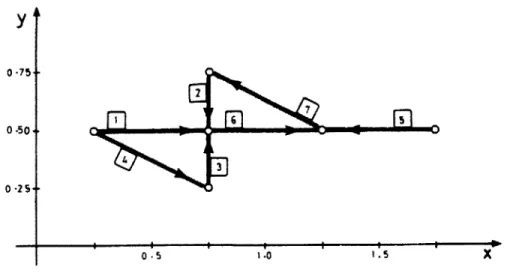
Consider F is a formex of the seventh order and the second grade and is in the form of

F = {[1, 2; 2, 2], [2, 3; 2, 2], [2, 1; 2, 2], [1, 2; 2, 1], [4, 2; 3,2], [2, 2; 3, 2], [3, 2; 2, 3]}

Let x and y be a function of every signet [S1, S2], and

x = (2S1-1)/4

y = S2/4

Let x and y be the center of each circle in a two-dimensional Cartesian coordinate system,

and every cantle of F be presented by a straight line joining the little circles that

correspond to its signets. And let the arrow-head be place on the line and indicated the

order of the appearance of the signets in a cantle. Also, label every line by the orderate of

the cantle. The resulting configuration is in Figure 3.2.1. It is referred to as a plot of F. FORMEX PLOTS

y

FIGURE 3.2.1: PLOT IN TWO DIMENSIONAL CARTESIAN COORDINATE SYSTEM 1

We can repeat the same procedure but now the center of each circle will be changed due

to the function as follows:

x = 2S1+S2-3 y = 3 S2-1

The resulting configuration is shown in Figure 3.2.2, which is another plot of

y

4.0 4

2-0 4

-4 -~

2.0 1 .0 6.0 X

FIGURE 3.2.2: PLOT IN TWO DIMENSIONAL CARTESIAN COORDINATE SYSTEM 2

i

.75

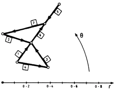
.50-Now we can repeat the same procedure but using a polar coordinate this time. And the

center of each signet will be given by the polar coordinates

r = S1/5

0 = (2 S₂-1)/10

The resulting configuration is shown in Figure 3.2.3.

e

0

CHAPTER FOUR FORMEX FUNCTIONS

4.1 Introduction

In scalar algebra, a relation such as

y = x2 _{+ 2x +1}

establishes a rule which is used to evaluate y for any given x. The general equation can

be represented by

y =f(x)

The term f is referred to as a 'function', so y is a function of x. The same rule here

applied to the formex functions. In a formex function, a relation such as

F = (D| G

established a rule which is used to evaluate F for any given G. This rule is representated

by a symbol, say D. That is, F is defined by G using the equation in D. And the symbol

'|' is referred to as the 'rallus symbol' and is read as 'rallus' or 'of'. As one needs to

process the same equations repeatedly, it would be more convenient and faster to

standardize the process into a function. The name of the formex functions reflects its

formex plot. A number of frequently useful formex functions for double-layer grids are

described in this chapter.

In discussing the formex functions, the following terminology and notation are used:

(1) If F and G are two formices and

then G can be also expressed in terms of F. In this case, the function is said to

have an 'inverse'. The inverse of a function (D is denoted by (D-1 and can be written as

G = <D-1 |F

(2) A composite function obtained from repeated application, say m times, of a

function <D is denoted by D 2. Thus,

(D |<(D | G is written as (D 2| G and (D-1|<D-1|: G is written as (D-2|: G

(3) A composite function that consists of D" and VD is equivalent to q"~+n For example,

(D2| 3 G- 5 G and

(D' | D-3 G -0G' G

(4) The zeroth power of any function <D is referred to as an 'identity function' and is

expressed as

G = <DO: G

The functions that are introduced in this thesis belong to the three families of formex

functions.

First, there is the family of 'transflection'. There are five basic classes of functions in

this family, and they are translation, reflection, vertition, projection and dilatation

functions. Any combination of these basic functions is referred to as a transflection.

Secondly, there is the family of 'introflections'. This family consists of three functions,

and they are recision, regular variant and absolute recision functions.

Thirdly, there is the family of 'cordations' consisting of four classes of functions that are

known as nexum, luxum, conexum and coluxum functions.

In this chapter, translation functions and reflection functions are discussed. All other

functions which are not discussed follow the same concept by changing the relationships

between F and F'.

4.2 Translation functions

F = {[4, 2, 0; 0, 3, 5], [4, 6, -9],[30, 4, -9]}

and one wants

G = {[4+3, 2,0; 0+3, 3, 5], [4+3, 6, -9], [30+3, 4, -9]}

which means G is a function of F by adding 3 units to the first signet of each cantle of

formex F. This relationship can be described in a translation function, and it is written as

G = tran(h,m) F

Where h is the direction or the order of the signet, m is the units need to be changed. In

replaced by 3. Any translation of the empty formex is considered to be the emplty formex itself. For example, if F1 = {[1, 2; 2, 2], [2, 1; 2, 2]} and if F2 =tran(1, 3)| F1, F3 = tran(2, 2): F2 and F4 = tran(1, -3)| F3

then F2, F3 and F4 are found to be

F2= {[4, 2; 5, 2], [5, 1; 5, 2]} F3 = {[4, 4; 5, 4], [5, 3; 5, 4]}

F4 =

{[1,

1.

The formex plot of F1 to F4 is shown in Figure 4.2.1, where the plot of Fi is denoted by

Pi. Ul shows the first direction and U2 shows the second direction of each cantle.

U2 4 3 2 1

*TI'P

Further examples, Fl = [2, 2; 1, 1], F2 = [12, 1; 12, 2], F3 = [12, 9; 11, 10] and F4 = [1, 10; 2, 10]

and where F5 to F9 are obtained as

F5= 8tran(1,i)

I

I

j)|

I

In order to get F5, F1 is obtained. F1 is called as a 'generant'. Thus, F2, F3 and F4 are

the generants of F6, F7 and F8. And F9 is obtained by 4 generants, namely F5, F6, F7

The formex plot of F1 to F9 are shown in Figure 4.2.2, where the plot of Fi is denoted by Pi.

U2

8

6

2

\

3

2

4

6

8

10

12

AN EXAMPLE OF FORMEX PLOT OF TRANSLATION FUNCTION2

The relationship between the plots of Figure 4.2.2 are seem to be the same rule described

for the plots of Figure 4.2.1. Thus, a translation function tran(h,m) gives rise to a

translation by m units in the Uh direction.

The basic properties of translation functions are as the following:

(1) Translation functions are commutative. That is,

P5

(2) The inverse of a translation function tran(h, u) is the translation function

tran(h, - u). That is,

tran(h, u)-1IF = tran(h, -u)IF

(3) tran(h, u')Itran(h, u)IF = tran(h, u+u')IF and this in turn implies that tran(h, u)'I F = tran(h, iu)IF

where i is an integer.

4.3 Reflection functions

F is a formex of rth grade, so F is in the form of {c1, c2, c3, c4,....., cr}. Let F' be a formex of the same grade, F' = {c'1, C'2, C'3, C'4,... cr}, and every cantle of F' is replaced by every

cantle of F where all values of i = 1, 2, 3, 4, ,r except for i = h, so

I'i = Ii, and

I'h, = 2u-lh

Where h is any nonzero integer from 1 to n, u is either an integer or semi-integer, such as

1, 1.5, 2, 2.5, 3, 3.5....

The rule which is described here for F to transform into F' can be symbolized in terms of

a formex function. The function is referred as a 'reflection function', and is written as

ref(h, u)

So the relationship between F and F' can be written as

F' = ref(h, u)| F

Any reflection of the empty formex is considered to be the empty formex itself.

F1 = {[2, 0, -9], [0, 0, 0; 1, 1, 1]

and if

F2 = ref(2, 2) Fl

then F2 is found to be

F2 = {[2, 4, -9], [0, 4, 0; 1, 3, 1]}

The basic properties of the reflection functions are as the following:

(1) Reflection functions that correspond to different directions are commutative. ref(hi, ui) ref(h2, u2) IF = ref(h2, u2) I ref(hi, ui) F

(2) A reflection function is the inverse of itself. That is,

ref(h, u)-1 F = ref(h, u)I F

This can imply and prove for the following.

ref(h, u)2w I F

=ref(h, u)" F * ref(h, u)| F

= ref(h, u)-w| F * ref(h, u)w| F =ref(h, u)0|F =F and ref(h, u)2w+l F =ref(h, u)2 w F *ref(h, u) I F

=ref(h, u)| F *ref(h, u) I F

= ref(h, u)

I

CHAPTER FIVE

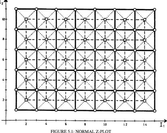
A double-layer grid structure consists of two interconnected parallel networks. As shown

in Figure.1, the top grid is indicated by full lines, the bottom grid is indicated by broken

lines, and the diagonal bars which connect them are indicated by dotted lines. The

structure consists of 280 beam elements that are rigidly connected together at 83 joints.

Suppose that the grid is to be subjected to analysis using the standard stiffness method in

conjunction with a computer program and that it is necessary to prepare the necessary

input data. For this purpose, one has to provide information about the interconnection

pattern, geometric particulars, material properties, external loads and support conditions.

I2

2--~ I I . I ~

i 2 4 5 N 10

FIGURE 5. 1: NORMAL Z-PLOT

12 14

A major part of the data consists of a description of the interconnection pattern of the

structure, thus we focus one attention on this particular aspect of data preparation.

The interconnection pattern of the structure may be described using the concepts of

formex algebra. Consider only the top grid for now. Focusing on the left bottom corner

of the top grid, an element such as ei can be described by the cantle

[1, 1; 3, 1]

This specifies that joint j1 is connected to joint

j2

by the cantle

[3, 1; 5, 1]

The combination of element ei and e2 can be represented by the construct

{ [1, 1; 3, 1], [3, 1; 5,1]} which is an example of a formex.

Using the method described above, one may now describe each individual element or

their combinations in terms of formices. For example,

F1= [1, 1; 3, 1]

and

F2= [3, 1; 5, 1]

represent the elements ei and e2, respectively, and

F12 = {[1, 1; 3, 1], [3, 1; 5, 1]} represent the pairs of elements ei and e2.

To obtain a formex representing the combination of the elements ei and e2, one may also

which is an example of formex composition.

More example,

F3= [1, 5; 1, 7]

and

F4= [1, 7; 1, 9] represent the element e2 e3 and e4, respectively.

If

F = F1 # F2 # F3 # F4 then this may be written as

. _Fi

which is an example of libra construction.

The above formex F is written as

F= {[1, 1; 3, 1], [3, 1; 5, 1], [1, 5; 1,7], [1, 7; 1, 9]}

Another way to show F is to use the 'formex function'.

tran(1, 1):

is a 'formex function' implying 'translation' in the first direction by 1 unit.

The symbol '| ' is called the 'rallus symbol' and has the role of separating the function

from its argument. For instance,

F2 = tran(1, 2): F1

F3 = tran(1, 2): F1 and

Now, let it be required to write a formex representing the combination of F1, F2, F3, F4, F5,

F6 and F7 (representing ei, e2, e3, e4, e5, e6 and e7).

6

. tran(1,2i)

I

where F = [1, 1; 3, 1].

Translation of F by zero unit in the first direction is F itself. That is

tran(1, 0)| F =F.

A translation function may imply translation not only in the first direction but also in the

second direction. For instance, now the top layer grid parallel to the I1 axis maybe

described by the formex

5 6

Ei= tran(2,2j) . tran(1,2i)

I

j=0 i=0

where F is equal to [1, 1; 3, 1], and the top layer grid parallel to the 12 axis maybe

described by the formex

7 4

E2 . tran(1,2i) . tran(2,2j)

I

i=0 j=0

where G is equal to [1, 1; 1, 3].

Let us consider now the third direction of the cantle. The interconnection pattern of a

double-layer grid is represented by a homogeneous formex of the third grade and second

plexitude in which each cantle represents an element of the grid. Furthermore, the

parallel to the I1-12 plane and intersects the 13 axis at 13= 1. So the third index of a signet

in the formex of the top grid is always equal to 1, and 0 for the bottom grid.

Formex plots that represent double-layer grids can be shown in the style of Figure 5.1 or

Figure 5.2. Figure 5.1 is called as a 'normal Z-plot', and Figure 5.2 is called as an

'oblique Z-plot'. An oblique Z-plot is used when some of the elements of the grids are

coincides in its normal Z-plot. The term Z-plot is used to refer to either a normal Z-plot

or an obliqueZ-plot. 12 10 8 -. 4 I I I I I I I I I I I I 6 8 1012 14 ₁₁

FIGRUE 5.2: OBLIQUE Z-PLOT Now E1can be described by

E2can be described by

E2 = . 4 tranid(2i,2j) 1 [1,1,1;1,3,1]

i=0

j

Furthermore, the bottom layer grid, which is parallel to the I1 axis can be described by

E3 5 4 tranid(2i,2j) |[2,2,0;4,2,0]

i=0 j=0

And the bottom layer grid, which is parallel to the I2 axis can be described by

6 3

E4 . . tranid(2i,2j) | [2,2,0;2,4,0]

STATIC ANALYSES OF DOUBLE-LAYER GRIDS

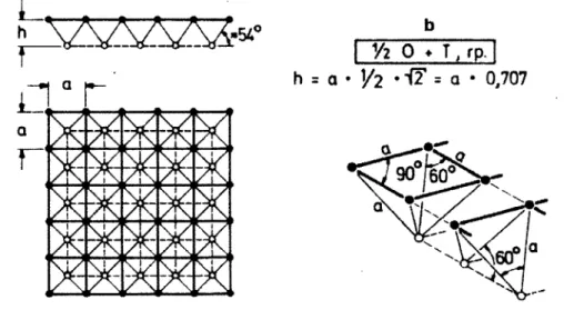
6.1 Geometry

Space structures are typical examples of skeleton frameworks. They consist of a large number of simple modular, prefabricated units, often of standard size and shape, which combine into a light, but very rigid, three-dimensional structure. In order to have standard size and shape units, the geometry of the double-layer grid roof needs to be carefully determined.

The double-layer grids in this thesis are based on squares. The top grid is offset from the bottom grid in plan but has the same direction. The grids are connected by diagonal members. The square is 1 by 1 meter and the diagonal is also 1 meter.

L

b

h -5e.

hh 0 +T

,

h =a - 2 -F2= a 0,707

I X1

FIGURE 6.1: GRID GEOMETRY

6.2 Structural Analysis

The distributed load of 30 psf(equal 1.4KN per square meter) is applied as point loads at each joint of the top grid. The structure is supported at its four corners. The loads are

0.35 KN at the four corners; 0.7 KN is at the other joints along the sides; 1.4 KN placed

at the rest of the joints on the top grid. All elements have only axial loads since the structure is considered to be a space truss.

In the finite element method, truss elements can be represented as 2-node, 3-node and 4-node elements. In this example, a 2-4-node element was employed since 2-4-node elements are adequate for modeling a truss. When the material is linear elastic, the 2-node truss element requires only 1-point Gauss numerical integration for an exact evaluation of the stiffness matrix, since the strain is constant in the element. In this example, steel pipes were used as the structural members. Analyses were carried out using 2 programs,

ADINA and SAP.

The double-layer grid structure is supported at the four corners with hinges that constrain translation. In this example, one should compare the forceRR stressRR and strainRR of each element and the displacement of each joint. Since stress RR is equal the product of the inverse of the cross sectional area and the force, we will consider only force and displacement here. This also applies to strainRR.

The first example is a 5 by 5 meter double-layer grid. When we model it in ADINA and

SAP, we find that the forces in each element are very similar. Since the structure is

symmetric, we expect the answers to be the same. We do not have to make the

calculation by hand using the method of joints, since it is time consuming and not very efficient.

The second example is a 2 by 2 meters double-layer grid. We could use the method of joints to find the force in each element. If we compare the forces from the method of the

2 joints and ADINA, we observe that they are almost the same2

6.3 Numerical solution

In the case of the 2 by 2 grid, the elements on the side carry zero force. The diagonals that connect directly to the support are subjected to tension. The rest of the diagonals are

In the case of the 5 by 5 grid, the elements on the side carry small compression. The diagonals that connect directly to the support carry extremely high tensile force. On the bottom grid, the side elements carry the second highest tension of the structure. The tensile force decreases with distance from the edge toward the interior. With respect to translation, the inner joints always have more deflection than the outer joints.

DESIGN OF A SPACE TRUSS ROOF

7.1 Geometry

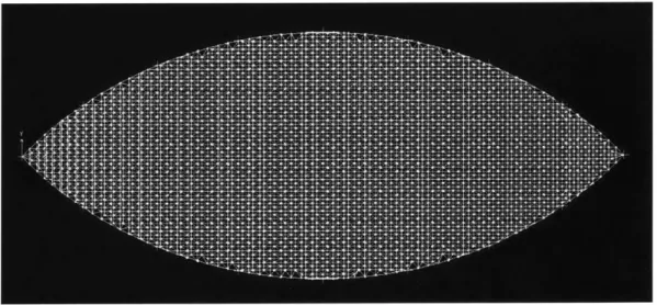
The elevation view of the space truss is an arc with a radius of 80 feet. By dividing the

angle of the arc, we can cut the arc into many equal length units. Basically the

double-layer grids are based on squares. The top grid is offset from the bottom grid in plan but

remaining directionally the same. The grids are connected by diagonal members. The

square is 3 by 3 feet and the diagonal is also 3 feet.

7.2 Structural Analysis

FIGURE 7.2.1: PLAN VIEW OF THE STRUCTURE IN SAP

There are more than ten thousand elements in each roof-truss, and because of the

only axial loads going through. The roof is supported by the steel columns, which

support the whole structure. These steel columns take the diaphragm loads. After

analyzing the structure, a 3-inch pipe with the thickness of 0.6 inches was chosen for the

columns. A few members have irregular length. But more than 30 thousand elements

will be produced in the same size making the design very economical3

1I(UUK 1.2.2: hLEVATIUN VIhW IN NAL'

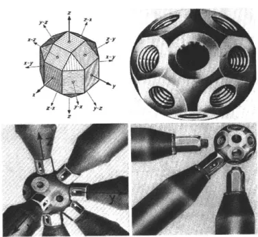
7.3 Mero System

Mero was invented by Dr. Max Mengeringhausen. The principle of the system is the

prefabrication and standardization of the element, which makes Mero economical.

Standard Mero connectors have 18 screw holes. This connector has 18 surfaces

connecting angles of 45, 60, 90 and multiples of these angles. It may be made in

faces, but special Mero connectors can be made, with holes drilled at special angles to

suit particular applications. The minimum angle between two adjacent holes is 35

degrees.

Z

FIGURE 7.3.1: A STANDARD MERO CONNECTOR

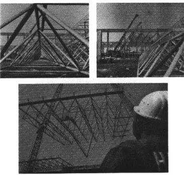
The issue of safety in a fire is important when using a space truss. In case of fire,

collapse of double-layer grids is commonly characterized by the sequential failure of

individual members. As fire develops, temperatures increase and the progressive

weakness of steel causes failure of members. After collapse of some parts of the

structure, the remaining sections are stable and still able to resist the applied load.

The erection of the Mero space system does not produce any special problems. Basically,

level, and then, with the help of simple lifting gear, hoisted up into their final position

and connected together, forming the final structure. The large amount of labor required

for normal assembly will be reduced through the erection of sizable parts at ground level.

Additionally, the usual high cost of renting the hoisting equipment is minimized, as the

cranes are used only when their load-carrying capacity can be exploited to the fullest, to

lift up very bulky or heavy parts.

CHAPTER EIGHT

Over the last century, engineers have been striving to build larger structures with less

material and less cost. Space structures have the incredible rigidity and ability to cover

large spans with minimum weight. Double-layer grids belong to the family of space

structure. The complex and regular nature of double-layer structural grids require the use

of computer techniques for the design and production.

When a structural system is to be analyzed by a digital computer, it is necessary to

provide a complete description of the system in an appropriate form. This constitutes the

data that are to be used in conjunction with a program. Data preparation is normally a

straightforward process involving nothing more than a systematic recording of known

facts. For large and complex systems, it is more difficult to control the input data.

Formex algebra may be used in different ways to overcome the difficulties of data

preparation. In particular, the description of the interconnection pattern of a structural

system may be conveniently formulated through the concepts of formex algebra.

Formex plots and formex functions are a set of rules extended from formex algebra to

minimize the work of data preparation. The concept of formex algebra can be applied not

only in double-layer grids but also in other engineering disciplines since it is a

mathematical system. This thesis demonstrated how the input data of a complex

geometry form, consisting of double-layer grids and described by many nodes, can be

reduced to only one equation by using formex formulation.

The last two chapters of the thesis focused on the analysis of double-layer grids. A

structure is that each element takes only axial loads. Each element of the double-layer

grid carries load differently depending on the support condition of the entire structure. A

square based double-layer grid supported on its four corners is the special case. The sides

of the structure carry relatively small compression. The diagonals that connect directly to

the support carry the highest tensile force. And the further the element is from the

SAP2000

to

or

May 14,1999 11:55

SAP2000

Mo 1

0

SAP2000

May 14 1999 11:52

May 141999 11:52

a w cn 0 - 0 0 0 wE 1 a. u

-e

Z

.

SAP2000

.74

I

SMay,14

Z

May 141999 11:47

SAP2000

0.000

1001

M0.

0<)

45

0.000

I / / I, / / I cO/ / I I / / / A A / / // - / - / / (\J/ ~-~" / / / / N< x a w co C>,~ Q ou i-0 0 0U

z

5

ADINA: AUI version 7.2.2, 14 May 1999: * NO HEADING DEFINED *** Licensed from ADINA R&D, Inc.

Finite element program ADINA, response range type load-step: Listing for zone WHOLEMODEL:

POINT X-DISPLACEMENT Time 0.OOOOOE+00 Node 1 0.0OOOOE+00 Node 2 0.OOOOE+00 Node 3 0.OOOOOE+00 Node 4 0.0OOOOE+00 Node 5 0.OOOOOE+00 Node 6 0.0OOOOE+00 Node 7 0.OOOOOE+00 Node 8 0.OOOOOE+00 Node 9 0.OOOOE+00 Node 10 0.OOOOOE+00 Node 11 0.OOOOOE+00 Node 12 0.OOOOOE+00 Node 13 0.OOOOOE+00 Time 1.OOOOOE+00 Node 1 0.OOOOOE+00 Node 2 1.43386E-22 Node 3 0.OOOOOE+00 Node 4 3.38813E-21 Node 5 -2.35738E-06 Node 6 2.35738E-06 Node 7 0.OOOOE+00 Node 8 6.35275E-22 Node 9 0.OOOOOE+00 Node 10 -2.35738E-06 Node 11 2.35738E-06 Node 12 -2.35738E-06 Node 13 2.35738E-06 *** End of list.

ADINA: AUI version 7.2.2, 14 May 1999: * NO HEADING DEFINED *** Licensed from ADINA R&D, Inc.

Finite element program ADINA, response range type load-step: Listing for zone WHOLEMODEL:

POINT Y-DISPLACEMENT Time 0.000E+00 Node 1 0.OOOOE+00 Node 2 0.OOOOOE+00 Node 3 O.OOOOOE+00 Node 4 0.OOOOE+00 Node 5 0.OOOOOE+00 Node 6 O.OOOOE+00 Node 7 0.OOOOOE+00 Node 8 0.OOOOOE+00 Node 9 O.OOOOOE+00 Node 10 O.OOOE+00 Node 11 0.OOOOOE+00 Node 12 0.OOOOOE+00 Node 13 0.00000E+00 Time 1.OOOOOE+00 Node 1 0.OOOOOE+00 Node 2 2.35738E-06 Node 3 0.OOOOOE+00 Node 4 6.35275E-21 Node 5 6.35275E-22 Node 6 6.35275E-22 Node 7 0.OOOOOE+00 Node 8 -2.35738E-06 Node 9 0.OOOOOE+00 Node 10 2.35738E-06 Node 11 2.35738E-06 Node 12 -2.35738E-06 Node 13 -2.35738E-06 *** End of list.

ADINA: AUI version 7.2.2, 14 May 1999: * NO HEADING DEFINED *** Licensed from ADINA R&D, Inc.

Finite element program ADINA, response range type load-step: Listing for zone WHOLEMODEL:

POINT Z-DISPLACEMENT Time 0.OOOOOE+00 Node 1 0.OOOOOE+00 Node 2 0.0OOOOE+00 Node 3 _0.000E+00 Node 4 0.OOOOOE+00 Node 5 0.OOOOOE+00 Node 6 0.OOOOOE+00 Node 7 0.OOOOOE+00 Node 8 0.0OOOOE+00 Node 9 0.OOOOE+00 Node 10 0.OOOOOE+00 Node 11 O.OOOOOE+00 Node 12 O.OOOOOE+00 Node 13 0.0OOOOE+00 Time 1.0OOOOE+00 Node 1 0.OOOOOE+00 Node 2 -1.83359E-05 Node 3 O.0OOOOE+00 Node 4 -2.00030E-05 Node 5 -1.83359E-05 Node 6 -1.83359E-05 Node 7 0.OOOOE+00 Node 8 -1.83359E-05 Node 9 0.OOOOOE+00 Node 10 -1.33351E-05 Node 11 -1.33351E-05 Node 12 -1.33351E-05 Node 13 -1.33351E-05 *** End of list.

ADINA: AUI version 7.2.2, 14 May 1999: * NO HEADING DEFINED *** Licensed from ADINA R&D, Inc.

Finite element program ADINA, response range type load-step: Listing for zone WHOLEMODEL:

Element field variables are evaluated using RST interpolation.

POINT STRESS-RR Time 1.0000E+00 Element 1 of Int point 1 Element 2 of Int point 1 Element 3 of Int point 1 Element 4 of Int point 1 Element 5 of Int point 1 Element 6 of Int point 1 Element 7 of Int point 1 Element 8 of Int point 1 Element 9 of Int point 1 Element 10 of Int point 1 Element 11 of Int point 1 Element 12 of Int point 1 Element 13 of element group 1 1.00370E-14 element group 1 -1.00370E-14 element group 1 1.65017E+02 element. group 1 1.65017E+02 element group 1 4.44692E-14 element group 1 -4.44692E-14 element group 1 -4.44692E-14 element group 1 4.44692E-14 element group 1 1.65017E+02 element group 1 1.65017E+02 element group 1 -4.44692E-14 element group 1 4.44692E-14 element group 1

Int point 1 Element 15 of Int point 1 Element 16 of Int point 1 Element 17 of Int point 1 Element 18 of Int point 1 Element 19 of Int point 1 Element 20 of Int point 1 Element 21 of Int point 1 Element 22 of Int point 1 Element 23 of Int point 1 Element 24 of Int point 1 Element 25 of Int point 1 Element 26 of Int point 1 Element 27 of Int point 1 Element 28 of Int point 1 -1.65004E+02 element group 1 -1.65004E+02 element group 1 -1.65004E+02 element group 1 -1.65004E+02 element group 1 4.95012E+02 element group 1 -1.65004E+02 element group 1 -1.65004E+02 element group 1 -1.65004E+02 element group 1 -1.65004E+02 element group 1 -1.65004E+02 element group 1 4.95012E+02 element group 1 -1.65004E+02 element group 1 -1.65004E+02 element group 1 4.95012E+02 element group 1 -1.65004E+02

Element 31 of element group 1

Int point 1 3.30033E+02

Element 32 of element group 1

Int point 1 3.30033E+02

ADINA: AUI version 7.2.2, 14 May 1999: * NO HEADING DEFINED *** Licensed from ADINA R&D, Inc.

Finite element program ADINA, response range type load-step: Listing for zone WHOLEMODEL:

Element field variables are evaluated using RST interpolation.

POINT STRAIN-RR

Time 1.OOOOOE+00

Element 1 of element group 1 Int point Element 2 Int point Element 3 Int point Element 4 Int point Element 5 Int point Element 6 Int point Element 7 Int point Element 8 Int point Element 9 1 of 1 of 1 of 1 of 1 of 1 of 1 of 1 of Int point 1 Element 10 of Int point 1 Element 11 of Int point 1 Element 12 of 1.43386E-22 element group 1 -1.43386E-22 element group 1 2.35738E-06 element group 1 2.35738E-06 element group 1 6.35275E-22 element group 1 -6.35275E-22 element group 1 -6.35275E-22 element group 1 6.35275E-22 element group 1 2.35738E-06 element group 1 2.35738E-06 element group 1 -6.35275E-22 element group 1

Int point 1 Element 15 of Int point 1 Element 16 of Int point 1 Element 17 of Int point 1 Element 18 of Int point 1 Element 19 of Int point 1 Element 20 of Int point 1 Element 21 of Int point 1 Element 22 of Int point 1 Element 23 of Int point 1 Element 24 of Int point 1 Element 25 of Int point 1 Element 26 of Int point 1 Element 27 of Int point 1 Element 28 of Int point 1 Element 29 of Int point 1 -2.35720E-06 element group 1 -2.35720E-06 element group 1 -2.35720E-06 element group 1 -2.35720E-06 element group 1 7.07160E-06 element group 1 -2.35720E-06 element group 1 -2.35720E-06 element group 1 -2.35720E-06 element group 1 -2.35720E-06 element group 1 -2.35720E-06 element group 1 7.07160E-06 element group 1 -2.35720E-06 element group 1 -2.35720E-06 element group 1 7.07160E-06 element group 1 -2.35720E-06 element group 1 4.71476E-06

Element 31 of element group 1

Int point 1 4.71476E-06

Element 32 of element group 1

Int point 1 4.71476E-06

ADINA: AUI version 7.2.2, 14 May 1999: *** NO HEADING DEFINED *** Licensed from ADINA R&D, Inc.

Finite element program ADINA, response range type load-step: Listing for zone WHOLEMODEL:

Element field variables are evaluated using RST interpolation.

POINT FORCE-R Time 1.OOOOOE+00 Element 1 of Int point 1 Element 2 of Int point 1 Element 3 of Int point 1 Element 4 of Int point 1 Element 5 of Int point 1 Element 6 of Int point 1 Element 7 of Int point 1 Element 8 of Int point 1 Element 9 of Int point 1 Element 10 of Int point 1 Element 11 of Int point 1 Element 12 of Int point 1 Element 13 of element group 1 3.01111E-17 element group 1 -3.01111E-17 element group 1 4.95050E-01 element group 1 4.95050E-01 element group 1 1.33408E-16 element group 1 -1.33408E-16 element group 1 -1.33408E-16 element group 1 1.33408E-16 element group 1 4.95050E-01 element group 1 4.95050E-01 element group 1 -1.33408E-16 element group 1 1.33408E-16 element group 1

Int point 1 Element 15 of Int point 1 Element 16 of Int point 1 Element 17 of Int point 1 Element 18 of Int point 1 Element 19 of Int point 1 Element 20 of Int point 1 Element 21 of Int point 1 Element 22 of Int point 1 Element 23 of Int point 1 Element 24 of Int point 1 Element 25 of Int point 1 Element 26 of Int point 1 Element 27 of Int point 1 Element 28 of Int point 1 -4.95012E-01 element group 1 -4.95012E-01 element group 1 -4.95012E-01 element group 1 -4.95012E-01 element group 1 1.48504E+00 element group 1 -4.95012E-01 element group 1 -4.95012E-01 element group 1 -4.95012E-01 element group 1 -4.95012E-01 element group 1 -4.95012E-01 element group 1 1.48504E+00 element group 1 -4.95012E-01 element group 1 -4.95012E-01 element group 1 1.48504E+00 element group 1 -4.95012E-01

Element 31 of element group 1

Int point 1 9.90099E-01

Element 32 of element group 1

Int point 1 9.90099E-01

SAP2000

SAP2000

-t

I

I

771

T

REFERENCES

Nooshin, Hashyar. Formex Configuration Processing in Structural Engineer. Elsevier Applied Science Publishers, London and New York, 1984

Makowski, Z. S. Analysis, design and construction of double-layer grids. Applied Science Publishers Ltd, 1981

Nosshin, Hashyar. Formex Data Generation in International Symposium-Innovative Applications of Shells and Spatial Forms. Oxford & IBH Publishing Co, 1988

Nooshin, Hashyar. Basic Concepts of Formex Configuration Processing, International Symposium on Membrane Structures and Space Frames, Osaka, Japan, September 1986. Disney, Peter. Formian: The programming Language of Formex Algebra in Shells, Membranes and Space Frames, Proceedings IASS Symposium, Osaka, 1986, Vol.3. Elsevier Science Publishers B.V., Amsterdam, 1986

Ik Nang Anna Cheah. Formices and Plenices in Structural Analysis and Design in Shells, Membranes and Space Frames, Proceedings IASS Symposium, Osaka, 1986, Vol 3. Elsevier Science Publishers B.V., Amsterdam, 1986.

Bathe, Dlaus-Jurgen. Finite Element Procedures Simon & Schuster / A Viacom Company, Upper Saddle River, New Jersey, 1996