DEZISION RULES FOR THE AUTOMATED GENERATION OF SrORAGE STRATEGIES IN
DATA MANAGEMENT SYSTEMS by
GRANT N SMITH S.B., MIT
(1974)
SUBMITTED IN PARTIAL FULFILLMENT OF THE REQUIREMENTS FOR THE
DEGREE OF MASTER OF SCIENCE at the MASS&AHUSETTS INSTITUTE OF TECHNOLOGY June, 1975 Signature of Author ... ... ... . Alfred P. Sl1oan'- chool otjAnageggp, May 9, 1 5
Certified by..-.. .. - . ... .. , ,...
/7 . Thesis Supervisor
Accepted by . . .s.. ... ... . .... * ... *.* . * .o .0
Chairman, Departmental Committee on Graduate Students
RC-HIVES
JUN 13 1975
DECISION RULES FOR THE AUTOMATED GENERATION
OF STORAGE STRATEGIES IN DATA MANAGEMENT
SYSTEMS.
by
GRANT N SMITH
Submitted to the Alfred P. Sloan School of Management on May
9, 1975 in partial fulfillment of the requirements for the
degree of Master of Science.
Current methods of determining storage strategies (both
logical and physical) rely usually on (1) expert opinion,
and (2) the experience of the designers. There has been
some work in the area
of automated design, but the
approaches taken to date generally apply only at generation
time, thus leaving the resulting design in
effect for the
rest of the life of the system. Should usage of the system
change over time, as experience shows that it will, large
inefficiencies may result owing to the original choice of
storage strategy.
The work presented here attempts to introduce dynamic
decisions regarding storage strategies that will be invoked
(1) on a regular basis, and (2) when system performance
degrades below an unacceptable
level.
These decisions
involve both the structure of the data base (such as which
fields are to be in
which files), as well as indexing, data
encoding, factoring and virtualizing decisions. Decision
rules are described which achieve this result.
Also described is a procedure whereby any given request will
be most efficiently satisfied, making use of the current
structure of the data base, indexes, etc.
Finally, the set of decision variables required to drive the
above decision subsystems is specified in detail.
Thesis Supervisor: Stuart E. Madnick
Assistant Professor of Management Science
Title:Acknowledgements
I wish to thank Professor Stuart E. madnick for his invaluable advice, comments and criticism throughout not
only the writing of this thesis, but through all the years in which I have been so fortunate as to be associated with
him.
In everyone's life, there is one eternal optimist. In mine, that is Professor John Donovan. He has been a powerful
motivating force throighout this work.
Last, but by no means least, thanks are due Chip Ziering for many hours of fruitfull - often heated - discussion.
Introduction... . . a...**..* .... * .* ...
The Relational Model of Data...
Shared Data Bases and User Flexibility.. Decision Variables and Truth Functions..
The Structural Decision Subsystem...
... Page
... Page
... Page
... *.Page
... Page
The Request Decision Sub Scenario for application
Decision Rules... conclusion.. .. . ... References. . .. . . . . .. .. Bibliography... system.. of .. .. .. .. ... ... Page 108 ... Page ... Page ... Page ... Page 126 145 151 152 Appendix 1... Appendix 2... Appendix 3... 6 15 37 53 68 ... . .Page .Page .Page 156 167 177 .... * ... 00
* .. eO..e. .. * .. . . S S SS S S * SS 5555*B*O * *05S5S~**. .SSSO .3.55.5 *55. * S S. * S 55 * Se. * 55 * 55 SeS 550 * S 55 *050 5550 55.5 0555 0S05 * 535 * 055 5.55 555550*05 OS S 505000 055050055 550505555 55 5005505 5.5555555 *05055505 55 *O.S**5 SSSsSS 555 55 5555 35 5 SL L 6ZL1 8 ti E ti ti~ 91t dsajnbT~ go
Is-0
* a * &SS B &S *SS 0 0 5 055 0 0. . . . . . . . . . . 00 , 0a L "L 9 *L C~ L Z. L Li *fI E IE t OE L eJ S Z!)YdIntroduction.
For some years nos- the concept of data-independent
applications programming has been expounded. What was
primarily at stake was the avoidance of rewriting of applications programs if and whenever the underlying data base was changed. Involved was a mapping from the logical data structure (as the data structure available to the
applications program came to be known) into some machine oriented data structure (or the physical data structure), the idea being that the system would take care of this mapping- function. Then, if there were any change in the physical structure, the mipping function would be changed so that the same logical structure as existed before this change would still be presented to any applications programs, and, in fact, any user (be it in the form of programs, or a person generating requests against that logical data structure). Note that throughout we shall use the term user to mean either a program or a person. It is not necessary for our purposes to distinguish between these two classes, since as far as the database is concerned, all
ZHAPTER I
requests look alike.
Arising from this approach is a division of responsibility,
and thus of expertise. The logical structure of the data is in the domain of responsibility of the user, while the physical structure and tha mapping function previously also in the domain of the aser, have now been removed. This is in
fact a desirable featire as the user may concentrate efforts on applications-oriented problems rather than becoming
bogged down in the technicalities of establishing a data base.
However, that is not guite the way things turned out. There were several attempts to design systems which would perform the mapping function ini handle the physical structures for the user, given the logical structure. But the way it turned out was that the mapping capabilities tended to be
rather simplistic in Zoncept and execution, with the result
that the user had to be quite knowledgable about the
physical structure (and thus the mapping function). Furthermore, no differentiation of responsibility was
generally delineated and so the user (or user group) now took on the responsibility of both the logical- and physical
structures. True, for any one logical structure the user now had a choice of physical structure coming from a wider range than personal experieice might previously have allowed, but
whether that was a blessing or a disguised horror remains
unclear.
Other promises made - and not kept - about data independence
again revolve around the mapping function. Theoretically, a given physical structure should be able to be mapped into several logical structures, and vice-versa. This facility
has not been realized to any notable extent.
Furthermore, the primary purpose of data independence, namely the isolation of users from changes in the physical data structure, has not yet realized its full potential. Rarely, if ever, was the physical data structure altered once established. It was a Herculean task to implement any
one physical structure, and no one was about to go in and
tamper once it was working.
Any one physical-to-lagical structure mapping would generally be performel only once, and decisions as to what
CHAPTER I
it should be were male at one point in time, with a fixed perception as to the future uses of the data base. These
decisions were, and still are, made by people. Much of the knowledge on which these decisions were based was knowledge gained from experience, and so was more akin to an art than a science. However, some non-trivial subset of such decisions are indeed logical and rational, and so subject to
some measure of automition.
It would be inaccurate to claim that no attempt has been
made to take advantage of the structured nature of some of these decisions. On the :ontrary, there have been several efforts addressed to this task, and these efforts can be
divided (perhaps unfairly) into two major groups:
simulation-oriented decisions used prior to system generation to aid in structuring decisions. These
are notably static, one-time decisions made at the discretion of some person, and requiring substantial human intervention. The results of decisions made at that point were to be influential throughout the
life of the lata base. However, much credit is due
the effort to formalize some major aspects of the decision.
dynamic rules used continually throughout the life
of the data base to monitor system usage and
performance. The results of this monitoring effort would, again, reguire major human intervention in
their interpretation and acting upon. However, the important aspect of these efforts was in that they attempted to track the system on an ongoing basis.
Whether any iction was taken on these results was
questionable. 3nce again there arose the dilemma of
whether to tamper with a working (albeit
inefficiently) system.
This work is intended to draw on the invaluable insights gained over the years in dealing with such systems as
purport to provile data independence, and some
logical-to-physical structure mapping, and to propose a methodology for achieving some of the promises made earlier.
It is important to emphasize that this is a methodology since no one work could pretend to be all-encompassing. The
approach here will be to:
1) describe a system in which there is true data independence 3asel on a physical-to-logical mapping capability,
2) enhance this system with the ability to perform some of the better formulated decision tasks,
CHAPTER I PAGE 11
including the monitoring of system use and the dynamic reconfiguration of the physical data structures without alteration of the logical structures. Attention will also be paid to the
initial structuring decisions made at definition
time.
3) further enhance the system with decision
capabilities that are oriented toward the efficient satisfying of requests against the data base.
The work here revolves around the relational model of data.
This should not be construed to be a dismissal of all other
models (such as the network model) as inferior. The author's familiarity with the relational model and the existence of a well-defined set of theoretical rules that can be applied in the model were the motivating factors behind this decision. It should also be pointel out that the relational model as herein used has embellishments and alterations derived from various personal experiences and sources of the author. The responsibilities for any errors and inconsistencies in the model employed here should not necessarily be attributed to the well-known names behind the relational model; they may
Structure of Thesis.
Chapter II will introiuce the relational model as needed for
our purposes, and point out the differences, where
applicable, between this molel and that found in most of the
literature.
Chapter III will address itself to the methodology employed for achieving data independence.
Chapter IV presents a list of decision variables maintained by the system. Since there is a long list of statistical
information about system usage and performance required to support dynamic decisions regarding physical restructuring, a consistent set of rules has been developed for naming these decision variables.
Chapter V will address itself to the decision rules responsible for initial specification, and subsequent
dynamic reconfiguration of the physical data structures -the Structural Decisign Substga (or SDS), and chapter VI
CHAPTER I
will concern those decisions made dynamically about optimally satisfying requests made against the data base -the Reguest Decision Subsistem (or RDS).
Chapter VII presents i typical scenario, and those decision rules developed in Chapters V and VI will be applied to the scenario to demonstrate the effectiveness of the decision
rules.
Chapter VIII concludes the thesis with some remarks as to further possibilities that can, and perhaps should, be explored, as well as ways to expand the decision rules
utilizing a similar methololgy to that employed here.
Again, it must be pointel out that the decision rules developed in Chapters V and VI are situation specific (and certainly dependent on the implementation of Chapter III) and are clearly not universally applicable. They are intended to demonstrate a methodology and there is no intention of developing a comprehensive and universal set of
rules.
Finally, some familiirity with BNF (Backus-Normal Form) is
CHAPTER II The Relational |odel af Data.
Probably the major stumbling block in introducing the relational model is the terminology. The concepts underlying this approiCh are familiar to us all.
consider a regular report, or table that we have all seen at one time or another. In Figure 2.1 is such a table; a
convenient format for representing such data. The columns spell out the categories of data; the rows provide a value
for each category. Note that the rows and columns might well be interchanged without loss or alteration of meaning. For example, in Figure 2.1 we see the columns labelled 'dept#', 'description', etc. And there are 7 rows. No-one
has difficulty in interpreting the information in Figure 2.1, and this is essentially the relational model.
By convention in the relational model, we always label the
columns, and put the data in the rows (ie: horizontally) just as is the case in Figure 2.1 . Furthermore, the columns
are called domains, ani the column headings are thus domain names. This arises from the mathematical concept of a domain
Plant: White Plains, New York. Period ending: Aug 31.
Summari of -oerations (in 000's) Dppt# Descrittion La b3 r Spray Coating Filing Sanding Buffing Assemble and Pack 2990 5915 998 1637 5915 4788 Expense Actual 6464 12829 2590 3907 11275 8846 Budet 7103 13981 2190 5243 10750 8998 Difference (Actual-Budget) - 639 -1152 + 400 -1336 + 525 - 152 22243 45911 48265
Fi-aur_
2.
1
1 2 3 6 7 10 TOTAL - 2354CHAPTER II
as being a collection of objects (or numbers, or any other information-carrying item). When we choose a value from that collection we are choosing an item from that domain.
Notice that each row is created by choosing a single item from each of the six domains. Each row in the table is
called an entry. Notice also that the order of the entries
(rows) in the table is not important. We might just as easily put the 'total' entry at the top of the table, and then the departments in decreasing 'dept#' order. In fact, we lose no information if we shuffle the rows; it may be inconvenient to have the rows in random order (as it would
be, for example, in a telephone directory) but no
information is lost by a random ordering of the entries.
Now, if we were to interchange domains 1 and 2 of Figure 2.1 (ie: 'Dept#' and 'description') there would be no problem
provided we changed the domain names (column headings) as
well. But notice that the order of the domains within any
one entry must be the same as that in all other entries if
the table is to remain meaningful. Thus, the order of the
domains is important, while that of the rows is not.
PrimaEXr-Ks.
In Figure 2.1 we may observe that there can be only one entry in the table far any one value of 'Depti', and the same applies for 'description', while there is no reason for this to be the case in any of the other columns. In fact, in the 'labor' domain the value '5915' appears twice. Thus, given the value '5915' and told that it is in the 'labor' column of Figure 2.1, we can not determine from that
information alone which department it is that is meant. (If it is both departments, then there is no problem.) But,
given a value for 'Dept#', there is no ambiguity about any information relevent to that row. Eg: given Dept# = 2, we can uniquely determina all other values in the entry. Thus,
we say that 'Dept#' is a candidate £Rigary t§! for the
table; ie: for any value of 'Dept#' there is only one entry
in the table.
In the event that there is no such domain, then some combination of domains must be found that exhibit this
property; namely, given a set of values for that comination
CHAPTER II
domains is uniquely determinel.
A table need not hive a primary key, but it is often
advantageous from the standpoint of efficiency to do so. (In the relational model propsed by Codd, et. al. no relation
may contain two entries that are identical, and so there always exists some primiry key, even if it is a combination of all domains. This is not the case here, as can be seen in
the definition of the 'Join' operator in Appendix 2.)
Normalization.
Looking again at Figure 2.1, we notice that printed above the table is some idditional information, such as the 'Plant', and the 'Period' covered. We see also that there
are two columns unler the heading of 'Expense'; viz. 'Actual' and 'Budget'.
Since the relational model views the world as a set of tables, we must find some way to include that information in the table itself. As it now stands, it is not really part of
the informarion in the table; rather it is a form of table heading. Considering the fact that the 'Plant' and the PAGE 19
'Period' are printed at the top of the table, we may assume
that it is of some iiportance, and we further assume that there are other plants and other periods.
one course of action is to set up a distinct table for each plant/period combination, each having an identical format to
that of Figure 2.1 . This would result in a large number of
identical, yet distinct tables, and so a second course of
actioa suggests itself: set up a single table for all
plant/period combinations, and somehow distinguish entries as belonging to some specific plant and period. This can be done by simply adding two domains to Figure 2.1: 'Plant' and
'Period'.
Furthermore, we must find some way of incorporating the notion of 'Expense' into the two domains 'Actual' and
'Budget'. To do so, we might merely rename the domains
'Actual expense', and 'Buiget Expense'. The table now is as
appears in Figure 2.2 .
Notice, however, that the table contains two domains each
V. -~
Summary of Operations
(In 000's)
Plant Period Dept* DescErig2tion Labor
Spray Coating Filing Sanding Buffing Assemble and Pack 2990 5915 998 1637 5915 4788 Actual Expense 6464 12829 2590 3907 11275 8846 Budget Expense 7103 13981 2190 5243 10750 8998 Difference (Actual-Budget) - 639 -1152 + 400 -1136 + 525 - 152 W Plns 10/31 TOTAL 22243 45911 Figure 2. 2 W Plns W Plns W Plns W Plns W Plns V Plns 10/31 10/31 10/31 10/31 10/31 10/31 1 2 3 6 7 10 -2354
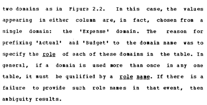
two domains as in Figure 2.2. In this case, the values appearing in either column are, in fact, chosen from a single domain: the 'Expense' domain. The reason for prefixing 'Actual' and 'Budget' to the domain name was to
specify the role of each of these domains in the table. In
general, if a domain is used more than once in any one
table, it must be qualified by a role name. If there is a
failure to provide suzh role names in that event, then
ambiguity results.
Use of a role name is not limited to cases in which a domain
is used more than on:e in the same table, and any domain
name may be qualified by a role name.
Figure 2.2 is a version of the table which has unique domain (or rather role) names, and is set up in such a way that it
contains all information in the table itself as opposed to some of it in the form of table headings. This is called a normalized table. In general, normalizing a table consists
of taking information that applies to all entries (such as the plant and perioi of Figure 2.1) and making it an
integral part of the entries themselves (as in Figure 2.2). More specifically, we take the primary key of tables higher
CHAPTER II
up in the hierarchy, ini make it part of the primary key of
the lower table. An example will help to clarify this point.
The example appearing in Figure 2.3(a) shows the logical view of the data that might exist in a corporate data base. Figure 2.3(b) is one form of a set of tables that might be
formed to store this logical view. Notice that some domains (such as 'children' in the 'employee' table) are not really domains, but the ames of other tables.
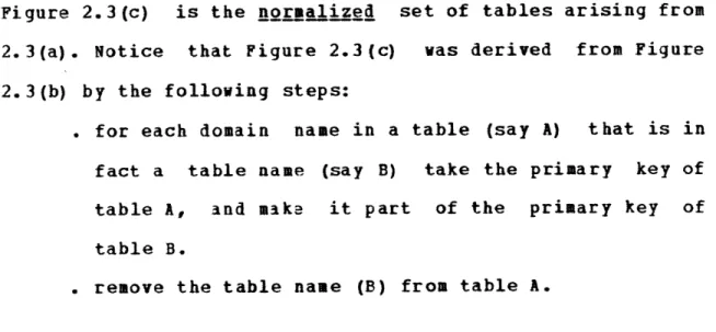
Figure 2.3(c) is the normalized set of tables arising from 2.3(a). Notice that Figure 2.3(c) was derived from Figure
2.3(b) by the following steps:
for each domain name in a table (say A) that is in
fact a table name (say B) take the primary key of table A, and make it part of the primary key of table B.
remove the table name (B) from table A.
This is the process of normalization, and, in the relational model, 111 tables must be normalized (ie: must not contain PAGE 23
EMPLOYEE (E MP. NAME, AGE)
JOBHIST (JOB.DATE,TITLE) CHILDREN (CHILD. NAME, AGE)
SALARY (SAL. DATE,SALARY)
1) EMPLOYEE (EMP. NAgAGEJOBHISTCHILDREN) 2) JOBHIST (JOB.DAT,TITLE,SALARY)
3) SALARY(SAL.DAfTSALARY)
4) CHILDREN (CHILD. VAgAGE)
laL
1) EMPLOYEE (EMP. NAMAGE)
2) JOBHIST (EMP. NAME, OB.DATgTIT LE)
3) S ALARY (E MP. NA ME, JB.ATE, _AL.DATE, SALAR Y)
4) CHILDREN(EM_.NAEg,ZHILDNAEi, AGE)
Fiqure 2.3
CHAPTER II
domain names that are in fact table names).
Why 'relational' model? What we have been calling tables are
call 'relations' in the relational model. This is more than an arbitrary name. Remember that we described above how an
entry is formed by selecting a value from each domain in the
table. In mathematical terminology, these entries are a
subset of all combinations of values, or a cartesian product of the domains. The name used for such a subset is a
'relation'.
More formally:
The cartesian product of A and B (written A X B) is a set of ordered pairs, each first element of the pair coming from A,
and each second element from B.
Ie: A X B = J(a,b):a(A, b<Bj ('4' means 'is a member of')
We can easily obtain an ordered n-tuple (where n>2) by this
method:
D1 X D2 X...X Dn = a(dl,d2,...dn): di Di, i=1,...nj
A relation will normally be written as a relation name PAGE 25
followed by an ordered, parenthesized list of domain names. le: R1(D1,D2,D3). For example: Employee(name,emp#,dept#).
The reader is referred to (3) for further discussion of relations and normalization.
Second Normal Form ani Functional Dependence.
The process of normalization described above (namely, the removal of all domain names that are in fact relation names) is adequate for most situations in which the user is careful to ensure that the domains asigned to the various relations are in fact assigned to the 'correct# relations. This is aided by the process of diagramming the data base as shown in Figure 2.3(a). However, there are times when what seems quite logical will, in fact, give rise to problems.
Consider Figure 2.1 , Notice that for any given value of
'Dept#' the value of 'description' is uniquely determined; or in other words, 'description' is functionally dependent on 'Dept#'. Clearly, in this case, the reverse is true as well; namely, 'Dept#' is functionally dependent on
CHAPTER II
'description', but this need not be the case.
Now, if for any reason we were no longer interested in Dept# 2 and therefor struck the second row from Figure 2.1, we lose the fact that Dept# 2 is 'coating'; ie: the
relationship (2,coating) loes not exist anywhere else. One way to avoid this is to establish a new relation containing only the functionally dependent domains (Dept#, description). We may now strike either of these domains from the relation in Figure 2.1 without loss of information.
These relations are said to be in second normal form; Ie: Domains not functionally lependent on each candidate key are
stored in a separate relation. Figure 2.1 would thus contain
'Dept#' as a domain, but not 'description', and another
relation now contains 'Dept#' and 'description'.
Third Normal Form and transitive dependence.
Third normalized relations are second normalized relations in which there exist no transitive dependencies.
If B is functionally dependent on A, and C is functionally PAGE 27
dependent on B, then by the algebraic transitivity laws, C
is also dependent on A. But in a somwhat different manner,
since it is also dependent on B which is dependent on A. In this case, we say that C is transitively dependent on A. This is true in any cise where the application of algebraic
transitivity yields an additional functional dependency, as it did in the above case.
Relations in third normal form would not contain any domains that were dependent on any other domain which is itself functionally dependent on some domain in the relation.
For the case above, where C is transitively dependent on A, we would establish a separate relation containing domains B and C, and remove C from the relation containing A.
It thus appears preferable to retain all relations in third normal form for the reasons outlined above.
The reader is referred to (4) for a more comprehensive treatment of second- and third normal forms.
CHAPTER II
Consider the existence of two relations: person (soc-sec, name, age), and
marriage(husband.soc_sec, wife.socsec)
Notice that 'person' contains the domain 'socsect and so does 'marriage'. Since 'marriage' contains that domain
twice, a role name is mandatory. Those supplied are:
'husband.socsec' and 'wife.socsecI. Now consider a
request to list the name and age of the wife of a person
with socsec 617-03-2911. This might be phrased (in some
arbitrary retrieval language) as follows:
list wife.name and wife.age for husband.socsec '617-03-2911' ;
Notice that the 'person' relation contains the domains referenced (viz: 'name' and 'age') but not the role name qualifier 'wife'. Intuitively, however, it is clear that the
information needed t3 satisfy the request is present, but not in any way that the system can utilize.
The way that the system mikes use of implicit information of the type in the example above is by transferring the role name qualifier 'wife' to the 'person' relation only for that
entry designated by the relationship between 'husband.socsec 617-03-2911' and the corresponding
'wife.soc-sec'. 'wife' loas not become a permanent role name qualifier in the 'person' relation.
Set Theoretic Notatil, Definitions and Examples.
In chapter I was mentioned the fact that a well-defined collection of theoretical rules exists which may be used to operate on relations (regardless of whether they are in any
particular normalizel form). This section outlines these
rules. This is perhaps where the model used here differs
most from those presented elsewhere(3,4). Differences will be pointed out at appropriate points in the discussion.
CHAPTER II 2peralion syabl Union U Intersection N Difference -Cartesian Produzt X Projection P Join * Composition Permutation M Compaction C Restriction R Division / Diadic/fj adi** Diadic Diadic Diadic Diadic Monadic Diadic Diadic Monadic Monadic Both Diadic
These operations are briefly described here, and are formally defined and examples given in Appendix 2.
** Diadic operators operate on two relations (they may both be the same relation); monadic operators operate on a single
relation.
Notation.
R<i> is the name of the i th relation
* means 'is a member of'
J....j implies a list, or set of the items between the
'Il's.
c(i) is the cardinality (number of entries) in R<i> n(i) is the degree (number of domains) in R<i>
d(i,j) is the j th domain of R<i>,
j=1,..n(i)
v(m)(ij) is the m th value of d(ij), m=1,..c(i) t(i) is an n(i)-tuple in R<i>
ie: t(i) (v (a) (i,1) , v(a) (ij2),..v(a) (i . n(i)) a 1,...c(i
L(jaI) is the length of list a
0 is the null set - ie: R<i>=0 implies c(i)=O asp means a is a subset of b (a=b is legal) acb means a is a prgaer subset of b (a b) Va means for all values of a
CHAPTER II
thesis.
Explanation of gperatars.
Union
The union of two sets consists of a set that contains all
entries that appear in eitter of the two sets. Intersection
The intersection of two sets is a set that contains only
entries that appear in both of the two sets.
Difference
The difference of two sets is a set that contains all
entries that appear in one of the sets, but not in the
other. Eg: If the two sets were A and B, then 'A - B' is a set of all entries that appear in A, but not in B.
Cartesian Product
This is as defined on Page 25
Projection
The projection of a relation is a procedure whereby some of the domains in the relation are removed.
Join
A join of two relations is the process whereby two relations may be combined into a single relation containing all the
domains of the two being joined.
Composit ion
This is the same as the join, except that the domain on
which the relations are joined is removed. This means that a
composition is in fact, a projection of a join. Permutation
A permutation appliel to a relation consists of merely re-ordering the domains in the relation.
compaction.
The compaction operator is used for deleting all redundent entries from a relation. It is used most commonly in conjunction with the projection operator, which may result in redundent entries.
Restriction
The restriction operator is used for selective retrieval from a relation.
Division
Division is the inverse of the cartesian product.
Introduction to XRN.
This section is intenled to be a very brief introduction to
the pertinent points about XRM.
XRM is a particular implementation of an n-ary relation data management model designed and built by IBM Scientific Center, San Jose (5). It operates basically as follows.
CHAPTER II
XRM can handle two types of information:
, character string data, and
. fullword (32 bit) numeric data
There are correspondingly two major subcategories of
relations; one that handles character strings, and another that handles n-tuples of numeric data. Any one relation type (character or numeri. n-tuple) can only handle data of that type.
Each entity in the system (character string, or n-tuple) is
automatically assigned an IRM ID when entered into the data
base. Given that ID, the entity can be rapidly and efficiently retrieved by XRM. And, given the entity, XRM
obtains its ID by applying a hashing function to that
entity, and then performing the retrieval. In the case of character strings, some number of the first bytes of the string are hashed; in the case of numeric n-tuples, all primary key domains are hashed.
All IDs in XRM are fullword integers.
In numeric relations (n-tuples), any domain can be inverted. PAGE 35
This is equivalent to building an index for that domain. Once such an inversion exists, given a value for that domain, XRN will rapidly find all ID's of n-tuples in the
relation that contain the given value in the inverted
domain. If no inversion existed, a linear search would be necessary. More is said about the implementation of
inversions in Chapter V.
For our purposes, this introduction will suffice. Additional
concepts will be explained as needed. For further
CHAPTER III
Shared Data Bases and User Flexibinlity.
This chapter presents a methodology based on the relational model for achieving independence between the logical- and
physical data structures.
One of the intentions of data independence is to allow the user to view the struCture existing in the data he (it) uses in a way most convenient for a specific application. This
means that the user should be provided with the facility to
define any relation containing any domains in any order, and be able to use it as such. Notice, however, some of the
issues raised by permitting this flexibility.
The most glaring problem arises as a result of the divergence from the concept of shared (or centralized) data bases. The benefits of shared data banks are many and have been adequately covered elsewhere, Now we are
proposing the facility for allowing every user a powerful tool that allows rapid and easy definition of relations for specific applications. What does this do to the centralized
data base concept? Each user now wants (and is able to PAGE 37
have) different relations for his application(s), which is
basically gaining effiziency and convenience at the expense
of generality. Each user must, furthermore, collect and
maintain his own data needed to support his application, rather than delegate that function to a central authority.
The traditional methal of centralizing data collection and maintainence has been the appointment of a data base
administrator whose responsibility it is to maintain the
central shared data base, and ensure that all users conform
to that data base. Zhinge to the data base is expensive and time consuming, and so generally to be avoided. User convenience was sacrificed in favor of a centralized data
base.
There is no need for sacrifice on either the user's part, or the data base administrator's part. This is where the
concept of a 1:n mapping of physical to logical structures demonstrates its value. There is no reason for denying a user a specific mapping from the single physical data base into a specific logical relation for some application. This presents no problem if the logical relation that the user
CHAPTER III
the domains existing in that physical data base. But what if the logical relation requires a mapping onto a domain that
does not yet exist in the physical data base, and is yet to
be created?
one possibility is to redefine the existing relevent relation in the physical data base to include the new
domain. Alternatively one could invoke the principle of a 1:n mapping, now from the logical to the physical relations,
and create a new relation containing the required
information.
We have thus expressed the need for a n:m mapping from logical to physical relations; ie: a logical relation can map onto several physical relations, and a physical relation
can be mapped into several logical relations.
Before proposing a methodology for implementing n:m mappings, let us iddress very briefly the issue of efficiency. In a very large data base, a user that constantly uses the same, small subset of data in a logical relation pays a high price in performing the mapping each
time. Some exception should be made in such a case whereby a physical relation is established containing that subset of data, and existing alongside the original physical
relations. This should not however be made to appear any
different to the user; the logical relation defined mast still appear to be the same and contain fully updated
information.
We turn now to a methodology.
Methodoloay.
There are basically three categories of relations that we have expressed a desire for in the above discussion:
physical relitions in the physical (centralized) data base,
logical (user defined) relations, and
special physical efficiency-oriented relations.
The terminology to be used here is as follows (and intended
to be consistent with the current terminology found in the literature):
CHAPTER III
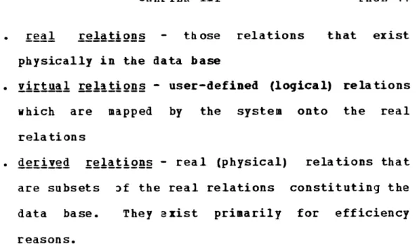
. real relations - those relations that exist physically in the data base
* virtual relations - user-defined (logical) relations
which are mapped by the system onto the real relations
. derived relations - real (physical) relations that
are subsets 3f the real relations constituting the data base. They exist primarily for efficiency
reasons.
We thus have a basic system as shown in Figure 3.1 . Notice that the elements of the system shown in Figure 3.1 interact in a specific way; more precisely, they form a hierarchy. Figure 3.1 can be easily reformatted to yield Figure 3.2. The same is true of all other figures in this chapter: they
can be expressed in an hierarchical relationship.
Notice also that this system has not eliminated either the
data base administrator or the need for some person (perhaps again the data base administrator) to specify the initial
real relations. The features of the system thus far are:
. the ability to define virtual relations on the
system maintained real relations, and have the PAGE 41
CHAPTER III
FiAure 3.2
system perform mapping functions (note that a virtual relation may in fact be identical to a real relation). More than one virtual relation may be defined on any one real relation.
. the ability to decide (the decision being made by
the data base alzinistrator) to create a (real) derived relation for reasons of efficiency in a
particular application
. the ability for a virtual relation to contain domains from more than one real relation.
As can be seen, the enhancements are concerned only with
the-system mapping functions. Thus, users may define virtual
relations consisting of domains in any (combination of) real relations, but may n2t define additional domains. It is
also important to point out the following:
. primary keys in virtual relations exist in the eye
of the user only; they do not necessarily correspond
to primary keys in real relations.
. the set-theoretiz operators defined in Chapter II are all that are required by the user for the creation of virtual relations, as virtual relations are a function only of existing relations. The data base adminstritor, however, who needs the capability
CHAPTER III
to define real relations and/or domains needs
additional facilities; perhaps in the form of a
DEFINE... or .REATE... command, not available to the
user.
Assuming a user wishes to define new real domains, these
additional real domaims will have to exist as real domains
in some real relation somewhere in the data base and there
is a decision required as to where in the data base this new domain will exist. Thus adding real domains (or real
relations) involves the user interacting with the data base adminstrator. The actions of the data base administrator in this situation would Zonsist basically of the following steps:
1) Determine from the user whether he is merely utilizing a iifferent name for some existing real domaia. If sa, simply tell the user to define a
synonym equating the two names.
2) If (1) is not the Case, apply some set of rules to determine in which real relation the domain(s)
belong(s).
3) Add the domain to that real relation, thus making it available for use in any user-defined virtual
relation. (Note that this step may require
restructuring some real relation. Alternatively, a
new real relation could be established consisting of the new domain, and the primary key of the real
relation that should contain that domain. A join is reguired each time the new domain is used. This decision must be made by the data base
administrator.)
Step (1) above appears to require some human intervention on the part of a person such as the data base adminstrator, who
is familiar with the global system and the existing real relations. But major portions of steps (2) and (3) can
indeed be formalized, and automated.
Provided there are same guidelines for the maintaining of real relations (eg: they must all be maintained in third-normal form - see Chapter II), then step (2) above can
be performed by the system.
In a similar way, by supplying some information as to the
expected use to be made of this new domain, the system can determine precisely haw to include this new real domain in
CHAPTER III
the data base - ie: parform step (3). Notice also that this
decision is directly analogous to that required in the creation of a derived relation.
0
Perhaps it would appear that all that is accomplished by the automation of the major share of steps (2) and (3) above is
the reduction of some administrative overhead. But consider
the capability of applying step (3) dynamically, which the
data base adminstrator does not have (except perhaps at predetermined, discrete time intervals). This means that the
real relations can be so structured as to reflect the
current system usage and requirements. Furthermore, because of the n:m mapping capability of the system, these changes in the real relations - be it mere addition of a real domain
or relation, or a restructuring of existing real relations -are not visible in any way to the virtual relations of the user. We may now modify Figure 3.1 to show the fact that there is some system funation controlling the structure of
the real relations in the data base; namely, the Structural Decision Subsystem (gQ). The modified version of Figure 3.1 appears in Figure 3.3 . If Figure 3.3 were reformatted into an hierarchical diagram, the SDS, which must be available to the real relation hanilers, would become the innermost level of the hierarchy.
CHAPTER III
We have discussed thus far in a non-technical manner a methodology for automating some of the functions revolving
around the maintainence of the real relations of the data
base.
Now, given a structure for the real relations of the data base (as specified by the SDS), and given also the possible
existence of derived relations (also determined by the SDS) it becomes clear that there may well be more than one way to
satisfy a request agiinst the data base. All requests from
users are against virtual relations (or some set-theoretic derivation of virtual relations), which from above, are mapped onto one or more real, or derived relations. Once
again some decisions are required in the mapping function to determine:
. whether the request is valid - ie: can logically
(and legally, from an access control point of view) be satisfied given the virtual relations involved, . how the request can be satisfied, and
. how best to satisfy the request.
The subsystem that controls these decisions is the Request Decision Subsystem (RD2). The RDS is responsible also for
determining how well it is doing in terms of efficiency. if the RDS decides thit system performance is degrading (perhaps as a result of changing system usage) it will
trigger the SDS in an attempt to restore performance to an acceptable level. We thus modify Figure 3.3 to include the RDS, as shown in Figure 3.4 . Its position in the corresponding hierarchical diagram is self-evident from this
figure.
The discussion in this chapter has purposely been non-technical in nature in an attampt to demonstrate the global functions and interactions within the system of the major decision subsystems - the SDS and RDS. Furthermore,
the techniques employed in implementing both the real- and virtual relations are of no consequence to the discussion, and have no impact on the methodology proposed.
Finally, notice that the real- and virtual relations are ilentical in their conceptual underpinnings, and thus requests against either are made in a consistent fashion. The requests used throughout will be in the format of set-theoretic operations on relations, be they real-,
CHAPTER III PAGE 51
D PLIONS
m on a" a -m a*N
defined in Chapter II.) This does not of necessity imply
that a user will employ set-theoretic requests directly; a mapping from a higher-level request language to a set-theoretic algebra is a well-understood, and conceptually simple operation. (See (6)) Thus our hierarchical view of Figure 3.4 might involve an additional layer between the
user and the virtual relations; namely, a request language -to - set theoretic operation mapping facility.
What we have presentel in this chapter is a methodology for
achieving true data independence and providing the user with powerful facilities for defining application-specific relations. At the same time, however, we preserve the centralized data base concept. The methodology is enhanced by two decision subsystems which assume some of the system structuring responsibility.
We proceed now to a detailed inspection of the decision subsystems.
CHAPTER IV Decision Variables and Truth Functions.
This chapter describes the naming conventions to be used in
subsequent sections for the naming of decision variables.
Since there is a rather large set of these decision
variables, it was decided to establish a consistent method for naming them. This method is presented here in BNF
(Backus-Normal Form) format, along with the appropriate
explanations.
Note that all decision variable names begin with a '$<number>'. This signifies the BNF rule number used to generate that name. A reference section containing these numbered rules appears as Appendix 3.
<relation
id> is an XRM-assigned internal ID; <domain #> is the position of a domain within a tuple.Rule# Rule
1 <qualifier>: := $1<relation type> <unit> <request>
<category>
<qualifier
type> <join info><options>
These are variables containing statictics about the use of domains in the capicity of qualifiers in the list of selection criteria that appear in a request.
<relation
type>::=<virtual>I<real>J<derived>
<virtual> ::= v<real> ::= r <derived> ::= d
<unit>: : =<doma in> I <relation>
<domain> ::= d(<relation id>,<domain#>) <relation> ::= r(<relation id>)
<request> ::= <retrieve>l<update>l<insert>l<delete> <retrieve> ::= r <update> ::= u <insert> ::= i <delete> ::= d <category>::=<siaple>l<compound> l<non-specific> <simple> ::= s <compound> ::= c <non-specific> : := n <qualifier type>::=<equality>g<nonequality> <unspecified> <equality> ::= e
CHAPTER IV
<noneguality>
::= n <unspecified> u <join info>::=<join>J<nojoin> <join> ::= j <nojoin> ::= n<options>: :=<null>I<index> I<no index>
<null>
::=<index> ::= i(trss) (trss='total
resloved set size')
<no index> ::= n
ExamPge: $lrd(i,j)rsen is the number of times the j-th domain of real relation i is used as a simple (ie: the only)
qualifier in a retrieval request, and was used as an
equality constraint. No join was needed to satisfy the
request.
The <relation type>,
<unit>
and <request> should be self-evident. For <category>, if there is only one domain in the list of selection criteria, then the <category> is 's'. In the event that there are several domains in the qualifierthe
<category>
is 'c, and if there is a sequentialretrieval from the relation, the
<category>
will be 'n' (or non-specific).For <qualifier type>, a constraint in a qualifier can be of essentially two types:
. an equality constraint, such as 'age=26',
. an inequality constraint, such as 'income > 20,000'. If there is no constriaint (as is the case when <category> is
'n') then the <gualifier type> is 'u' - or unspecified.
<join
info> will be a 'j' in the event that there was a join required in the reslowing of the request, and it will be 'n'if no join was necessiry.
<options>
will be null in the event that<category>
is 's'.If <category> is 'c', however, then <options> will show
whether some other domain in the list of qualifiers had n
inversion in the real relation. If so, then
<options>
is'i' - or 'index', and the system will also store the total
size of the resolved set (the set of entries that results
when those domains with indexes are used first in a
restriction). If there was no other domain in the list of domains in the selection zriteria, then <options> is 'n'.
CHAPTER IV
Rule# Rule
2 <retrieved object>::= <relation type>
<unit>
<request> <abject> <join info>This is a set of variables that will contain statistics as to the use of domains as the objects of a request.
<relation type>::=<real>j<virtual>l<derived> <real> ::= r
<virtual>
:=v<derived> ::= d <unit>::=<domain>J<relation>
<domain>::=
d(<relation id>,<domain #>)<relation> ::= r(<relation id>)
<request>::=<retrieve>i<update>I<insert>I<delete>
<retrieve> ::= r
<update> ::= u <insert> ::= i
<delete> ::= d
<object>::=
<simple> I <compund> I <entry>(<aggregate>)
<object>
<simple> ::= s <compound> ::= c <entry> ::= e <aggregate>::=SUMIAVIMAXIMINICOUNTIUNIQUE <join info>::=<join>I<nojoin> -<join> ::= j PAGE 57<nojoin> ::= n
Exampie 1) $2rr(i)rej is the number of times a whole entry is retrieved from real relation i, when a join
was necessary to resolve the request.
2) $2vd(i,j)r(AV)sn is the number of times that the average of the values in oly (since
<object>
is's') domiin
j
of virtual relation i is retrieved; no joins were needed to resolve the request.<object> in this rule is similar to
<category>
of rule #1. The value of<object>
will be s if this is the only domain specified for retrieval (or update) in the request. If there are several domains specified, then<object>
is 'c'.<object> may also be in
<aggregate>
if the individual itemswere not required, but some aggregation of them was.
Rule# Rule
3
<joins>::=
$3<relation
type><domain> <domain>
This type of variable maintains statistics about the
involvement of relations in joins. It specifies the number of times a relation was joined to some other relation by a
CHAPTER IV
<relation type> ::= <virtual>t<real>t<derived> <virtual> ::= Y
<real> ::= r <derived> ::= d
<domain>::= d(<relation id>,<domain #>)
Example: $3rd(i,j)d(k,m) is the number of times that relation i was joined by domain
j
to domain m of relation k.Rule# Rule
4 <system data>::=$4<system variable>
These variables store information about system parameters
and costs.
<system variable>::=<block size> I <index blocking
factor> I <cost-per-I/O> I <relation
blocking factor> I <cost/byte/day> <overhead per call to XRM> I
<time
period> <block size>::= p<index blocking factor> ::= bfx(<domain>)
<domain>::=<relation id>,<domain #> <relation blo.king factor> ::= bfe(<relation id>)
<cost-per-I/O>::= io
<cost/byte/day>:
:= sc<overhead
per call to XRM>::= opc<time
period>::= tIn XRM, bfx(i,j) is constant Vi,j, and bfe(k) is constant
Vk. So, for our purposes we can refer to them simply as 'bfx' and 'bfe'. The <time period> 't' will be the length of time since the last restructuring of the data base by the
SDS. All SDS decisions are based on the period since the
last restructuring occurred, and so decisions will be based on this time period.
Rule# Rule
5
<relation
data>::=$5<relation variable>These variables are used to store information regarding relations.
<relation
variable>::=<degree><type> I<degree> is th
<cardinality><type>
<degree>::= #d(<relation id>)
<cardinality>::= cy(<relation id>)
<type>: :=<real>I<virtual>I<derived> <real>::= r
<virtual>::= v
<derived>::= d (<method of derivation>) e number of domains in the relation;
CHAPTER IV
<cardinality> is the number of entries in the relation.
Rule# Rule
6 <domain data>::=$6(<domain name>)<domain variable> These variables are usel for maintaining statistics about
domains.
<domain variable>::=
<#
unique values><#
unique values> ::= qEramp1e $6(state)q is the number of unique values that will be found in domain 'state'. Notice that for domains that are numeric, $6(i)g is the same as the cardinality of the
relation in which domain i appears. For character strings, it may be anything from 1 to the cardinality of the relation in which it appears.
Rule# Rule
7 <user information>::=$7<user variable>
<user variable>: :=<response time weight factor> <response time weight factor>::=r
The
<response
time weight factor> is a user-suppliedpreference for how the response time is to be weighted in PAGE 61
structuring decisions. it is a value from 0 thru 1
inclusive. For purposes of this thesis, the value of $7r will be 0.5, which is essentially a null value. However,
the variable may be taken into account by merely appending
'$7r' to all cases where '$4io' and '$4opc' appear in the
decision rules, and by appending '(1-$7r)' to all instances of '$4sc' in the decision rules.
Truth functions.
In addition to the statistical variables above, these is a
set of truth functions used to test for specific conditions. The names of these truth functions all begin with: '$8'. The value of a truth function is '1' if applying the function to a spezifiz case is true; otherwise the value is '0'. For example, if T(i) were a truth function that tests for negativity, then if i<0, T(i)=1, otherwise
T(i)=0.
The truth functions employed here are presented below. (Note
that the <type> of a relation (real, derived or virtual) is
CHAPTER IV
$8d(ij) domain
j
appears in relation i$8i(j,k) domain k in relation
j
is inverted. (For virtualrelations, $8i(j,k)=0 always.)
$8p(i,j) domain j is one of the primary key domains of
relation i.
$8x(i)r relation i is a real relation.
$8x(i)d(<method>) relation i is a derived relation, and <method> is the method of derivation. If <method> did not involve a restriction, then
<method>::=<nill>.
$8n(i,j) domain j of relation i is mandatory. le: a value
must be proviled for this domain before an entry in
relation i will be made.
Note $8n(i,j)=1
*j
where $8p(ij)=1. (Primary key domains are mandatory.)$8u(j) domain
j
contains unique values (eg: socsec_#)$8r(i,j) same as $8n(i,j) except that it refers to a role name. Also notice that $8r(ij) is a subset of
$8d(i,j) Thus this is a truth function that tests
whether a role name is in relation i.
$8_(j)<data type><starage strategy>
<data type>::=<character> I <fixed> I <float> I <vector> I <bit>
<character>::=
c<fixed>::= x <float>::= f
<vector>::= t(<size>) <bit>::= b
<storage
strategy>::=<virtual> I <real encoded> I <real unencoded><virtual>::= v
<real encoded>::= e <real unencoded>::= u
This set of truth functions is to test the data type of
domain
j.
For exmaple, if $8_(name)ce=1 then domain 'name' is an encoded character string.$8f(ImI,lnI) is a truth function that tests whether each of the domiins in list Inl are functionally
dependent on the whole list ii.
Note 1) List Imi is not a list of all domains on which members of list ini are functionally dependent. Each n'4lnj may be functionally dependent on some 1xlx/Im also.
2) If In I=O (ie: is empty) then
$8f(ImlIni) =0.
$8m(lpi,iq) is a function that tests whether lists IpI and
CHAPTER IV
$8f(Ip ,PqP)=$8f(IqjqpI)=1, and also $8m(lpI,IqI)
implies $8m(IgI,Ip1).
Transitivity also holds: $8m(Jpgjgj)=$8m(Iqi,IsJ)=1
implies that S8m(ptIsI)=1.
$8c(IpI,g) (<function>) is a function which tests whether q (note that q is not a list) is computationally dependent on domains Ipl. For example, if domain q
is defined as Iq=6.3 * p' then q is computationally dependent on p. (<function>) is the computation
required to derive q from the list of domains Ipf.
$8od(k) is a truth function set up for a request. It is '1' if domain k appears as one of the object domains
in the request.
$8eq(k) is a truth function used in requests. It is '1' if
domain k appears as a qualifier with <qualifier
type> 'e'.
$8nq(k) is similar to $8eg(k) except that the <qualifier type> is not 'e'.
Note that truth functions may be implemented as unary and
binary relations (depending on the particular truth function) where existence of an entry in the relation signifies 'true', or '1'.
The complete list of iecision variables and truth functions that are used in this collection of decision rules is listed
in Appendix 3.
In addition, the following notation will be employed in
subsequent chapters:
. an '*' appearing in any decision variable name means
the sum of all the possible replacements of the **.
For example:
$lvd(i,j)*sej = $lvd(ij)rsej + $1vd(i,j)dsej +
$lvd(i,j)usej
($lvd(i,j)isej is not used.)
Or:
$lrd(i,*)rsej = SUM($lrd(i,k)rsej) for k=1,...$5#d(i) . a '' in a name means the product of all possible
replacements for the '%'. For example:
$lvd(i,j)rseg = $1v(i,j)rsen.$1vd(i,j)rsej
. a list between two * I' (vertical bars) means the sum
of that list. For example:
CHAPTER IV PAGE 67
The reader is advised to become familiar with the 7 rules and the various truth functions to avoid continual reference to Appendix 3 and thus to expedite reading.