Deep learning with physical and power-spectral priors for robust image inversion

Deep learning with physical and power-spectral

priors for robust image inversion

by

Mo Deng

B.S. Electrical Engineering, University of Illinois, Urbana

Champaign(2013)

B.S. Mathematics, University of Illinois, Urbana Champaign (2013)

S.M., Electrical Engineering and Computer Science, Massachusetts

Institute of Technology (2016)

Submitted to the Department of Electrical Engineering and Computer

Science

in partial fulfillment of the requirements for the degree of

Doctor of Philosophy

at the

MASSACHUSETTS INSTITUTE OF TECHNOLOGY

May 2020

c

○ Massachusetts Institute of Technology 2020. All rights reserved.

Author . . . .

Department of Electrical Engineering and Computer Science

May 15, 2020

Certified by . . . .

George Barbastathis

Professor of Mechanical Engineering

Thesis Supervisor

Accepted by . . . .

Leslie A. Kolodziejski

Professor of Electrical Engineering and Computer Science

Chair, Department Committee on Graduate Students

Deep learning with physical and power-spectral priors for

robust image inversion

by

Mo Deng

Submitted to the Department of Electrical Engineering and Computer Science on May 15, 2020, in partial fulfillment of the

requirements for the degree of Doctor of Philosophy

Abstract

Computational imaging is the class of imaging systems that utilizes inverse algorithms to recover unknown objects of interest from physical measurements. Deep learning has been used in computational imaging, typically in the supervised mode and in an End-to-End fashion. However, treating the machine learning algorithm as a mere black-box is not the most efficient, as the measurement formation process (a.k.a. the forward operator), which depends on the optical apparatus, is known to us. Therefore, it is inefficient to let the neural network to explain, at least partly, the system physics. Also, some prior knowledge of the class of objects of interest can be leveraged to make the training more efficient. The main theme of this thesis is to design more efficient deep learning algorithms with the help of physical and power-spectral priors.

We first propose the learning to synthesize by DNN (LS-DNN) scheme, where we propose a dual-channel DNN architecture, each designated to low and high frequency band, respectively, to split, process, and subsequently, learns to recombine low and high frequencies for better inverse conversion. Results show that the LS-DNN scheme largely improves reconstruction quality in many applications, especially in the most severely ill-posed case. In this application, we have implicitly incorporated the system physics through data pre-processing; and the power-spectral prior through the design of the band-splitting configuration.

We then propose to use the Phase Extraction Neural Networks (PhENN) trained with perceptual loss, that is based on extracted feature maps from pre-trained clas-sification neural networks, to tackle the problem of low-light phase retrieval under low-light conditions. This essentially transfer the knowledge, or features relevant to classifications, and thus corresponding to human perceptual quality, to the image-transformation network (such as PhENN). We find that the commonly defined per-ceptual loss need to be refined for the low-light applications, to avoid the strengthened “grid-like" artifacts and achieve superior reconstruction quality.

Moreover, we investigate empirically the interplay between the physical and con-tent prior in using deep learning for computational imaging. More specifically, we investigate the effect of training examples to the learning of the underlying

physi-cal map and find that using training datasets with higher Shannon entropy is more beneficial to guide the training to correspond better to the system physics and thus the trained mode generalizes better to test examples disjoint from the training set. Conversely, if more restricted examples are used as training examples, the training can be guided to undesirably “remember" to produce the ones similar as those in training, making the cross-domain generalization problematic.

Next, we also propose to use deep learning to greatly accelerate the optical diffrac-tion tomography algorithm. Unlike previous algorithms that involve iterative opti-mization algorithms, we present significant progresses towards 3D refractive index (RI) maps from a single-shot angle-multiplexing interferogram.

Last but not least, we propose to use cascaded neural networks to incorporate the system physics directly into the machine learning algorithms, while leaving the trainable architectures to learn to function as the ideal Proximal mapping associated with the efficient regularization of the data. We show that this unrolled scheme significantly outperforms the End-to-End scheme, in low-light imaging applications. Thesis Supervisor: George Barbastathis

Acknowledgments

It’s still hard to believe that this enjoyable journey is coming to an end. Many people, both in and out MIT have offered me indispensable help throughout this wonderful experience.

First and foremost, I would like to first thank my research supervisor, Prof. George Barbastathis, for the incredible patience he offered me when I first transitioned into the lab in 2016; his guidance that gradually shaped my philosophy of research; his dedication to teaching and research that reinforced my career plan as a professor like him. I am most impressed to the incredible open-mindness of George. He, coming from a physics background, bravely embraced the opportunity that the tide of machine learning offered and tried to make machine learning more physics-aware, and thus, more efficient.

I would also like to thank Prof. Rajeev Ram and Prof. Frédo Durand for being on my thesis committee, your insightful questions during the committee meeting and your useful advice on the thesis.

Also, I would like to thank all of my peer colleagues in the MIT 3D optical systems lab, especially: Shuai Li, for being a knowledgeable and hardworking collaborator in many of my research projects; Alexandre Goy, who I see as a big brother/second mentor, for countless insightful discussions not only in the lab about research, but also on a broad spectrum of topics in history, current social issues and politics; Iksung Kang, for being a diligent and reliable collaborator on the experimental side; Kwabena Arthur, for your help on many of my manuscripts; Subeen Pang (a.k.a. Fresnel Gibbs) for the discussions on the scattering theory. And, on the Singapore side, to Zhengyun Zhang, Maciej Baranski, and Weina Li for taking care of me during the wonderful summer of 2018 that I spent there and the discussions that we had.

I would like to also thank my collaborators outside our lab, including Prof. Peter So and his student Baoliang Ge at MIT; Prof. Renjie Zhou and his student Yanping He at the Chinese University of Hong Kong; Prof. Demba Ba at Harvard and his graduate students Bahareh Tolooshams and Andrew Song. Moreover, I would like to

thank Prof. Zuowei Shen and Hui Ji at National University of Singapore, for useful discussions during the summer of 2018.

At MIT, last but not least, I would like to thank Prof. Pablo Parrilo for being a nice academic advisor. I will always remember the semester that I TAed for your optimization class; Ms. Irina Gaziyeva for her help on countless administrative mat-ters; and Janet Fischer as well as Prof. Leslie Kolodziejski, from the EECS graduate office for their constant help throughout the years and especially their assistance and consulting during my transition to George’s lab.

Equally importantly, I would like to thank all my family members, especially: My grandparents, both university professors who devoted all their careers to their students; and in their retirement years/ my early days, cultivated the deepest respect to science and passed on your precious values and characteristics to me.

My dad, from his unique perspective as an outstanding artist, keeps motivating me to be the best in my community, and exemplifies the importance of maintaining the passion in the career. My mom, whose strict words are always betrayed by her deep love and pride for me.

One of the greatest turning points to my life took place when I met my love Mengran in March of 2016, at the time when my Ph.D. journey hit its valley. Your unyielding love for me, even in the most difficult time, has made me believe there is light even at the end of the infinite corridor. Our beautiful daughter Noah, I am sure, is the most precious gift both you and I have ever received.

This doctoral thesis has been approved by the following thesis

committee:

Professor George Barbastathis . . . .

Research Supervisor

Professor of Mechanical Engineering

Professor Frédo Durand . . . .

Thesis Reader

Professor of Electrical Engineering and Computer Science

Professor Rajeev Ram . . . .

Thesis Reader

Professor of Electrical Engineering and Computer Science

Contents

1 Introduction 25

1.1 Computational imaging as an inverse problem . . . 25

1.1.1 Data-fidelity term . . . 27

1.1.2 Regularization . . . 28

1.2 The use of deep learning in computational imaging . . . 30

1.2.1 Basic of machine learning algorithms and the fully-connected neural networks . . . 30

1.2.2 Convolutional neural networks and their applications in com-putational imaging . . . 34

1.3 Thesis outline . . . 36

2 Learning to synthesize: splitting and recombining low and high spa-tial frequencies for full-band image recovery 41 2.1 Motivation . . . 41

2.2 Preliminary work— DNNs trained with examples with spectral pre-modulation . . . 43

2.3 Methodology of learning to synthesize by DNN (LS-DNN) . . . 46

2.4 Results . . . 51

2.4.1 Low-noise image super-resolution in diffraction-limited imaging under incoherent illumination . . . 51

2.4.2 Low-noise quantitative phase retrieval . . . 57

2.4.3 Quantitative phase retrieval under low-light conditions . . . . 59

3 Perceptual loss trained Phase Extraction Neural Networks

(PLT-PhENN) for phase retrieval at low photon budget 73

3.1 Using VGG-based perceptual metrics for better image quality . . . . 74

3.2 Perceptual loss-trained PhENN (PLT-PhENN) for phase retrieval at low light conditions . . . 78

3.2.1 The reconstructions at ReLU-22 trained PhENN and the fre-quency signature of the artifacts . . . 79

3.2.2 Probing shallower or deeper: finding an optimal ReLU for artifact-free, high-quality reconstructions . . . 85

3.3 Discussions and future work . . . 90

4 On the interplay between physical and content priors in deep learn-ing for computational imaglearn-ing 99 4.1 Introduction and Motivation . . . 99

4.1.1 Two important questions in deep learning . . . 99

4.1.2 Phase retrieval and the weak object transfer function (WOTF) for lensless phase imaging . . . 100

4.1.3 Generalization error in machine learning . . . 102

4.2 Entropy as a metric of the strength of the regularization effect imposed by a training set . . . 103

4.3 Results on synthetic data . . . 105

4.3.1 Performance of cross-domain generalization under different train-ing datasets . . . 105

4.3.2 How well has PhENN learned the physics model? . . . 108

4.4 Experimental Results . . . 112

4.4.1 Optical Apparatus and pre-processing . . . 112

4.4.2 Comparisons of the cross-domain generalization performance . 114 4.4.3 Star-pattern experiment to demonstrate the learning of the propagation model . . . 115

5 Towards high-speed, real-time optical diffraction tomography based on single-shot angle-multiplexing interferogram with deep learning 119

5.1 Introduction . . . 119

5.1.1 Mathematical foundation of angle-scanning ODT . . . 121

5.1.2 Reconstruction based on multi-scattering model – reconstruc-tions based on beam propagation method . . . 122

5.2 High-speed limited-angle ODT with deep learning . . . 123

5.2.1 From preliminary Rytov reconstruction to full-angle reconstruc-tions (n2n). . . 124

5.2.2 From limited-angle true phase maps to 3D refractive index maps.125 5.3 Towards fast, real-time ODT from a single-shot angle-multiplexing in-terferogram based on limited number of angles. . . 129

5.3.1 Single-shot angle-multiplexing interferogram . . . 130

5.3.2 Different strategies to the ultimate goal . . . 133

5.4 Reconstruction assessment in optical diffraction tomography . . . 136

5.4.1 Using direct predictions on micro-beads as reconstruction as-sessment . . . 137

5.4.2 Assessment based on the discrete dipole approximation (DDA) 138 5.4.3 Assessments to take place in our project . . . 138

5.5 Future work . . . 139

6 Cascaded neural networks for algorithms unrolling 141 6.1 Learning to regularize: proximal learning for phase retrieval under low light conditions . . . 141

6.1.1 Problem Formulation . . . 141

6.1.2 Proximal gradient descent algorithm . . . 145

6.1.3 Neural Proximal gradient descent algorithm for linear inverse problems . . . 147

6.2 Proximal gradient descent for nonlinear inverse problems . . . 148

6.3.1 Deep convolutional exponential auto-encoder . . . 152 6.3.2 Application: blind deconvolution under Poisson contamination 154 6.3.3 Application: learning for optimal structured illumination for

Poisson-contaminated phase tomography . . . 156 6.4 Future work . . . 158

7 Conclusions and Future work 159

7.1 Conclusions . . . 159 7.2 Future work . . . 162

A Supplementary results on LS-DNN for image recovery 165

A.1 Resolution test of LS-DNN . . . 165 A.2 Comparison of LS-DNN reconstructions with the perceptual-loss trained

List of Figures

1-1 General scheme for computational imaging systems. (Figure reprinted from [1] with permission). . . 26 1-2 The schematic of LISTA. X: input data. The mutual inhbition matrix

𝑆 = 𝐼 − _𝐿1𝑊_𝑑𝑇𝑊𝑑 and the filter matrix 𝑊𝑒 = _𝐿1𝑊𝑑𝑇 are based on the

underlying dictionary matrix 𝑊𝑑, and are learned. . . 31

1-3 The schematic of fully-connected neural networks. This figure is adopted from the MIT 6.869 (taught by Prof. Bill Freeman and Prof. Antonio Torralba). . . 33 1-4 Multi-layer convolutional neural network: generic scheme. Figure reprinted

from [1] with permission. . . 33 1-5 Convolutional neural networks. This figure is adopted from [2] with

permission. . . 34

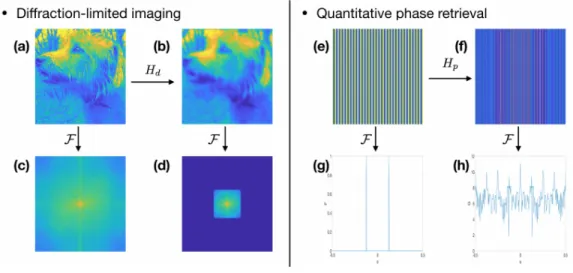
2-1 Effect of forward operators in the frequency domain. (a) an ImageNet example. (b) diffraction-limited measurement, (c) and (d) are the Fourier spectrum of (a) and (b), respectively. (e) A sinusoidal phase object. (f) Intensity measurement, (g) and (h) are 1D cross-sections along the horizontal direction for the Fourier spectrum of (e) and (h), respectively. . . 42 2-2 Log-log scale of power-spectral density of natural images. . . 43

2-3 Spectral pre-modulation. (a). Original image 𝑓 in ImageNet. (b). The spectrally pre-filtered image ˜𝑓 . (c). Fourier transform of original image 𝐹 (𝑢, 𝑣). (d). Fourier transform of the spectrally pre-filtered image ˜𝐹 (𝑢, 𝑣). Figure reproduced from [3] with permission. . . 44 2-4 The flowchart of PhENN trained with spectrally pre-filtered examples.

(a). the training stage. (b). the test stage. . . 45 2-5 Resolution of the original PhENN.(a) dot pattern example for the

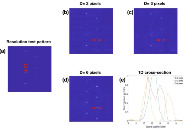
res-olution test. (b) PhENN reconstructions for dot pattern with D = 2 pixels. (c) PhENN reconstructions for dot pattern with D = 3 pixels. (d) PhENN reconstructions for dot pattern with D = 6 pixels. (e) 1D cross-sections along the lines indicated by red arrows in (b)-(d). Figure reproduced from [3] with permission. . . 46 2-6 Enhanced resolution of PhENN by the spectral pre-modulation. (a) dot

pattern example for the resolution test. (b) PhENN reconstructions for dot pattern with D = 2 pixels. (c) PhENN reconstructions for dot pattern with D = 3 pixels. (d) PhENN reconstructions for dot pattern with D = 6 pixels. (e) 1D cross-sections along the lines indicated by red arrows in (b)-(d). Figure reproduced from [3] with permission. . . 47 2-7 Reconstructions with ordinary and spectrally pre-modulated PhENN.

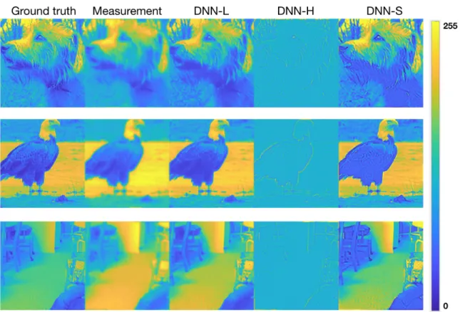
(a) ground truth for a phase object. (b). diffraction pattern captured by the CMOS (after background subtraction and normalization). (c). phase reconstruction by PhENN trained with original ImageNet ex-amples. (d). phase reconstruction by PhENN trained with spectral pre-modulated examples. Figure reproduced from [3] with permission. 48 2-8 Scheme for LS-DNN. (a). training stage (b). test stage. . . 50 2-9 LS-DNN for super-resolution in diffraction-limited imaging. From left

to right: ground truth; measurement (blurry image due to frequency hard cut-off); DNN-L reconstruction; DNN-H reconstruction; DNN-S reconstruction. . . 53

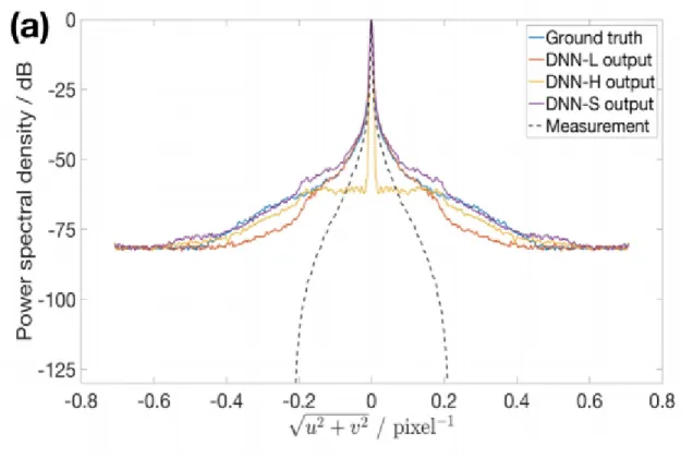
2-10 1D (normalized) PSDs of various elements in super-resolution in diffrac-tion limited imaging by LS-DNN . . . 54 2-11 Demonstration of vast improvement over VDSR using the LS-scheme. 55 2-12 Compare with LS-DNN and DNN-L-3 for image super-resolution in

diffraction limited imaging. . . 56 2-13 Comparison with DualCNN [4] . . . 56 2-14 LS-DNN for QPR with low noise. From left to right: ground truth;

intensity measurement; DNN-L reconstruction; DNN-H reconstruction; DNN-S reconstruction. . . 60 2-15 1D (normalized) PSDs of various elements of low-noise phase retrieval

by LS-DNN. . . 60 2-16 From top to bottom: ground truth image and its 2D Fourier spectrum;

noiseless Approximant and its 2D Fourier spectrum; Approximant for 1 photon/pixel illumination and its 2D Fourier spectrum. . . 63 2-17 Reconstructions by LS-DNN (top: 1 photon/pixel/frame, bottom: 10

photons/pixel/frame); from left to right: Approximant (the input to the LS-DNN system), DNN-L reconstruction [5], DNN-H reconstruc-tion (𝑞 = 0.5), DNN-S reconstrucreconstruc-tion, ground truth. . . 64 2-18 Fourier spectra of two test examples and their reconstructions from the

components of the LS scheme. . . 65 2-19 1D diagonal cross-sections of the average 2D power spectral density

(PSD) of test set images for 𝑝 = 1 photon per pixel. . . 66 2-20 Comparisons of LS-DNN reconstructions under different 𝑞′𝑠 for 𝑝 = 1

photon/ pixel. Columns from left to right: ground Truth and DNN-L output; DNN-H output under different 𝑞’s; DNN-S output under different 𝑞’s; 1D cross-section (along the dashed line indicated in the ground truth image) of (i) DNN-L output (green) (ii) DNN-S output under different 𝑞′𝑠 (blue dashed) and (iii) ground truth (red). . . 67

2-21 Comparisons of LS-DNN reconstructions under different 𝑞′𝑠 for 𝑝 = 10 photon/ pixel. Columns from left to right: ground Truth and DNN-L output; DNN-H output under different 𝑞’s; DNN-S output under different 𝑞’s; 1D cross-section (along the dashed line indicated in the ground truth image) of (i) DNN-L output (green) (ii) DNN-S output under different 𝑞′𝑠 (blue dashed) and (iii) ground truth (red). . . 68 2-22 PCC comparison of DNN-S, DNN-L and the Approximant. 𝑝 = 1

photon/pixel, 𝑞 = 0.5, for all test images. . . 69

2-23 Cross-domain generalization of LS-DNN. (a). Predicting MNIST ex-amples by ImageNet trained LS model; (b). Predicting ImageNet Ex-amples by MNIST trained LS model. . . 70

3-1 VGG network architecture [6]. . . 76

3-2 VGG-based feature loss in DNN training. . . 78

3-3 Comparison of reconstructions from PhENN trained with perceptual loss (ReLU-22) vs. NPCC [5]. The scaled-up images show that some details are not rendered by the NPCC-trained PhENN whereas they become clearly identifiable with the perceptual loss function. However, the “grid-like" artifacts are more prounced as the photon count gets lower. 80

3-4 (a) Reconstruction by the VGG16 ReLU-22 feature-loss trained DNN for the 1-photon level. (b) Log-scale magnitude of the 2D Fourier Transform of the reconstruction shown in (a). The artifact contributes in the modes indicated by the arrows. (c) Cross sections of the log-scale magnitude of the Fourier Transform of the perceptual loss reconstruc-tion (blue), corresponding to image (b), ground truth (black) and the NPCC-trained DNN reconstruction (red). . . 81

3-5 (a) Log-magnitude of the power spectral density of the test set of re-constructions ˆ𝑓 clearly showing the signature of the artifact, which is perceived in the reconstructions as a prominent network of horizontal and vertical strips, e.g. Figs. 3-3 and 3-4. (b) Horizontal profile of (a). (c) Vertical profile of (a). (d) Diagonal profile of (a). . . 82 3-6 Dependence of VGG16 loss on the frequency of the noise. (a) Diagram

showing the scanning scheme in the Fourier domain. The noise 𝑛 is added on at a single frequency and made Hermitian, i.e. 𝑛(𝜈𝑥, 𝜈𝑦) =

𝑛(−𝜈𝑥, −𝜈𝑦)*. (b) Loss as a function of frequency for the horizontal

scan and five examples from the test set, for a noise amplitude of 𝐴 = 0.1. (c) Loss as a function of frequency for the vertical scan for the same five examples. (d) Loss as a function of frequency for the diagonal scan for the same five examples. (e) Absolute value of the derivative of the loss with respect to frequency. The values are averaged over the 50 examples of the test set and plotted for the horizontal, vertical and diagonal scans. The ellipses in (c) and (d) indicate where strong non-smoothness can be observed in the loss curves. The position of the spikes correspond to artifact features observed in the spectrum of the average reconstruction. . . 92 3-7 Change in the frequency components of an image through the

mini-mization operation of Eq. (3.7). The frequency 𝜈 refers to position (𝜈𝑥, 𝜈𝑦) = (𝜈, 𝜈) in the Fourier domain (diagonal scan). The value

plotted is the difference of the modulus of the spectrum of the noisy image ˜𝑓 (defined in Eq. (3.4)) and the spectrum of ˆ𝑓 , the result of optimization Eq. (3.7) starting from ˜𝑓 . . . 93 3-8 Reconstructions (sub-figure (a)), scale-up of the region marked in (a)

(sub-figure (b)) with feature loss defined at various layers of VGG16 for 𝑝 = 1. In each sub-figure, Row (i): Approximant and ground truth from a representative sample; rows (ii) to (v) each contain layers before 1-Pooling, after 1-Pooling, 2-Pooling and 3-Pooling, respectively. . . . 94

3-8 PSDs of the reconstructions with feature loss defined at various layers of VGG16 for 𝑝 = 1. In each sub-figure, Row (i): Approximant and ground truth from a representative sample; rows (ii) to (v) each con-tain layers before 1-Pooling, after 1-Pooling, 2-Pooling and 3-Pooling, respectively. . . 95 3-9 Reconstructions by VGG19 feature loss trained PhENN . . . 96 3-10 Reconstructions and PSDs produced by mixed loss defined at various

layers of VGG19 . . . 97 4-1 Schematic plot of the lensless phase imaging system. . . 101 4-2 Entropy histogram of ImageNet and MNIST. Each histogram is

com-puted based on 1000 bins and 10000 images. . . 104 4-3 Cross-domain generalization performances of ImageNet-PhENN and

MNIST-PhENN on synthetic data. The defocus distance is 𝑧 = 100mm.109 4-4 Cross-domain generalization performances of ImageNet-PhENN and

MNIST-PhENN on synthetic data. The defocus distance is 𝑧 = 150mm.110 4-5 Comparison of LWOTFs-ImageNet, LWOTF-MNIST, WOTF-computed

and WOTF-theory. . . 111 4-6 Optical apparatus. HWP: Half-wave plate, OBJ: objective lens, SF:

spatial filter, CL: collimating lens, POL: linear polarizer, SLM: spatial light modulator, NPBS: non-polarizing beamsplitter, L: lens. . . 113 4-7 Phase modulation vs. 8-bit grayscale value for the experiments. . . . 114 4-8 Cross-domain generalization performances of ImageNet-PhENN and

MNIST-PhENN on experimental data. The defocus distance is 𝑧 = 150mm. . . 116 4-9 Reconstruction of the star pattern. (a). Intensity measurement at

𝑧 = 150mm. (b). star pattern (weak) object. (c). reconstruction by ImageNet-trained PhENN. (d). reconstruction by MNIST-trained PhENN. . . 117 5-1 General optical apparatus for ODT. . . 120

5-2 Learning tomography based on beam propagation method. The figure is reproduced from [7]. . . 122

5-3 Comparison of Rytov reconstructions, Tomocube reconstructions and LT-BPM reconstructions on micro-beads. . . 123

5-4 3D U-net architecture for n2n network. . . 125

5-5 The general schematic of n2n scheme. The input to the n2n network can be preliminary reconstructions based on 5 angles using Rytov ap-proximation, with or without TV regularization. . . 126

5-6 The n2n results of the micro-beads. Each sub-figure shows the x-y, x-z and y-z sections of the 3D refraction index map. (a) the cross-sections of the Rytov-ODT reconstruction results with 5 angles; (b) the cross-sections of the TV regularized Rytov-ODT reconstruction results with 5 angles; (c)the cross-sections of the TV regularized Rytov-ODT reconstruction results with all 49 angles, which is the ground truth we believed. (d)The output of the U-Net when we take fig(a) as the input and the MAE loss function; (e)The output of the U-Net when we take fig(a) as the input and the NPCC loss function; (f)The output of the U-Net when we take fig(b) as the input and the NPCC loss function. The scale bar is 10 𝜇m and the colorbar shows the value of retrieved refraction index. . . 127

5-7 The n2n results of HEK cells. Each sub-figure shows the x-y, x-z and y-z cross-sections of the 3D refraction index map. (a) the cross-sections of the Rytov-ODT reconstruction results with 5 angles; (b) the cross-sections of the TV regularized Rytov-ODT reconstruction results with 5 angles; (c)the cross-sections of the TV regularized Rytov-ODT re-construction results with all 49 angles, which is the ground truth we believed. (d)The output of the U-Net when we take fig(a) as the input and the MAE loss function; (e)The output of the U-Net when we take fig(a) as the input and the NPCC loss function; (f)The output of the U-Net when we take fig(b) as the input and the NPCC loss function. The scale bar is 10 𝜇m and the colorbar shows the value of retrieved refraction index. . . 128 5-8 Phase2RI 2D U-Net. . . 129 5-9 From 4 phase maps to refractive index maps. (a). the chosen

illumina-tion configuraillumina-tion on the Tomocube angle-scanning pad. The indices in red correspond to the angles used (b). the phase extracted from the respective interferogram. (c). x-y, x-z and y-z cross-sections of the reconstructions of HEK cells by the Phase2RI DNN versus the ground truth (49-angle Rytov reconstructions with TV regularization). (d). reconstructions versus the ground truth at different 𝑧’s. The 𝑧 dis-tances are with respect to the middle of the 𝑥 − 𝑦 slice of the sample and positive sign indicates the direction toward the detector. . . 131 5-10 Angle-multiplexing interferogram. Left: angle-multiplexing based on

four angles. Right: Fourier transform of the angle-multiplexing inter-ferogram. . . 132 5-11 Strategy 0: DNN that maps the K-angle multiplexing that . . . 133 5-12 Strategy I: single-shot interferogram → crude phase maps → 3D

re-fractive index maps. . . 134 5-13 Estimated crude phase maps from the angle-multiplexing interferogram.135 5-14 Reconstructions from strategy I: the CrudePhase2RI network. . . 136

5-15 Strategy II: single-shot interferogram → crude phase → corrected phase → 3D refractive index maps. . . 137 5-16 Phase correction results of the PhaseCorrection network. . . 137 6-1 Unrolled DNN schematic for Proximal Gradient Method for Inverse

Problems . . . 147 6-2 Comparison of reconstructions by the end-to-end, unrolled and the

Approximant schemes under 1 photon/pixel. . . 150 6-3 Comparison of reconstructions by the end-to-end, unrolled and the

Approximant schemes under 10 photons/pixel. . . 151 6-4 Quantitative comparison (PCC) of the reconstructions from the

End-to-End, Unrolled and the Approximant schemes under 1 photon/pixel. 152 6-5 Quantitative comparison (PCC) of the reconstructions from the

end-to-end, unrolled and the Approximant schemes under 10 photons/pixel. 153 6-6 Deep convolutional exponential-family auto-encoder (DCEA)

archi-tecture for exponential convolutional dictionary learning. The en-coder/decoder structure mimics the Convolutional Sparse Coding (CSC) step and the Concolutional Dictionary Learning (CDL) step. The en-coder performs T iterations of CSC. In the dictionary step, the dic-tionary H is updated through the backward pass. Figure reprinted from [8] with permission. . . 154 A-1 Resolution test for DNN-L, DNN-H and DNN-S outputs (𝑞 = 0.5).

(a). dot pattern with spacing 𝐷 = 4cm (ground truth) (b). DNN-L reconstruction. (c) DNN-H reconstruction (d) DNN-S reconstruction. (e).1D cross-section of the neighbourhood indicated by the red arrows in (a)-(d). . . 166 A-2 Comparison with perceptual loss strategy [9] for SR in DLI. . . 167

List of Tables

2.1 Quantitative comparison of reconstructions by Approximant, DNN-L and DNN-S, based on a test set of 500 images. Each entry takes the form of ’average ± standard deviation’. . . 66 2.2 Quantitative comparison of reconstructions by Approximant,

DNN-L-3 and DNN-S (for 𝑞 = 0.5), based on the test of 500 images. Each entry takes the form of ’average ± standard deviation’. . . 69 3.1 Quantitative assessment of reconstructions by feature loss PLT-PhENN

defined at various VGG16 layers. Each entry takes the form of average ± standard deviation. . . 88 3.2 Quantitative assessment of reconstructions by feature loss PLT-PhENN

defined at various VGG19 layers. Each entry takes the form of average ± standard deviation. . . 89 3.3 Quantitative assessment of reconstructions by mixed-loss PLT-PhENN

defined at various VGG19 layers. Each entry takes the form of average ± standard deviation. . . 90 4.1 Cross-domain generalization ability performance of PhENN trained

with ImageNet and MNIST, respectively, for 𝑧 = 100 mm (synthetic data). . . 107 4.2 Cross-domain generalization ability performance of PhENN trained

with ImageNet and MNIST, respectively, for 𝑧 = 150 mm (synthetic data). . . 107

4.3 Cross-domain generalization ability performance of PhENN trained with ImageNet and MNIST, respectively, for 𝑧 = 150 mm (experi-mental data). . . 115 5.1 Quantitative metrics of various reconstructions by the phase-to-refractive

index scheme, based on different configurations of 4 phase maps (with-out the center illumination) and 5 phase maps (with the center illumi-nation). . . 129 5.2 Quantitative metrics of various reconstructions by the phase-to-refractive

index scheme, based on the optimal illumination configuration and dif-ferent number of training examples. . . 130 5.3 Quantitative metrics of various reconstructions by the phase-to-refractive

index scheme, based on the optimal illumination configuration and dif-ferent number of training examples. . . 130 A.1 Resolution comparison for various reconstructions in LS-DNN. . . 166

Chapter 1

Introduction

1.1

Computational imaging as an inverse problem

Computational imaging (CI) is a class of imaging systems that delivers the the esti-mate of the object of interest in imaging, based on its indirect and imperfect mea-surement, with the help of the physical forward model associated with the imaging process and the prior information about the class of objects of interest.

Let 𝑓 denote the 2D or 3D object that we are interested in imaging. Intuitively, not all objects of interest (e.g. imaging transparent objects) can be directly measured with the camera, in then way that we take photographs in our daily life. Such difficulty necessitates the existence of the computational imaging (CI) systems, which consists of two components: the physics component, which produces the imperfect measurement of the object, based on the properties of the light illumination and the optics of the imaging system; and the inverse algorithm, where the object of interest is estimated from the measurements formed earlier. The physics component further breaks down to the illumination operator 𝐻𝑖, where the incident field interacts the

object and the collection operator 𝐻𝑐, that models the propagation of the light exiting

the object to the remainder of the optical system. The forward operator 𝐻, that maps the object to the physical measurement, is the aggregation of the illumination and

collection operator, i.e. 𝐻 = 𝐻𝑐𝐻𝑖, and the noiseless measurement

𝑔0 = 𝐻(𝑓 ) := 𝐻𝑓, (1.1)

where, for notation simplicity, we often neglect the parenthesis even when 𝐻 may be nonlinear.

The captured signal on the detector, 𝑔, however, is almost always contaminated by noise. The exact modeling of the formation mechanism of noise on the charge coupled devices (CCDs) is rather complicated. Here we simplify the modeling by categorizing the contributions of uncertainties in the signal into two categories, the shot noise and the readout noise. The shot noise arises due to the quantum nature of photons as they can only arrive at the detector in whole numbers and when collecting photons from an unvarying source over time, statistical fluctuation occurs and it largely follows the Poisson distribution and is signal-dependent. On the other hand, the readout noise, or readnoise, which is a consequence of the imperfect measurement of the voltage induced by the charges knocked free by photons, as part of the CCD operation. The shot noise is usually modeled as a Poisson variable and the readout noise is modeled as additive Gaussian random variable. Therefore, the contamination in the system is typically modeled as:

Figure 1-1: General scheme for computational imaging systems. (Figure reprinted from [1] with permission).

𝑔 =P {︂ 𝑝𝐻0𝑓 ⟨𝑔0⟩ }︂ +N , (1.2)

where 𝛽 = ⟨𝑔0⟩ is the mean of the noiseless measurement. Such normalization allows

𝑝 to be the average number of photons/pixel and N ∼ 𝑁(0, 𝜎2𝐼), where 𝜌 = _𝛽𝑝. The process of retrieving the object 𝑓 from the measurement 𝑔 is naturally for-mulated as the following computational inverse problem

ˆ 𝑓 =argmin 𝑓 𝐿{𝐻𝑓, 𝑔, Ψ(𝑓 )} =argmin 𝑓 𝐷(𝐻𝑓, 𝑔) + Ψ(𝑓 ), (1.3)

where 𝐷(·, ·) is the data-fidelity term to constrain the reconstruction to be consistent with the system physics; and Ψ(·) the data-fidelity term to express our prior knowledge about the class of objects of interest (assuming the regularization coefficient has been incorporated into Ψ(·)).

However, solving (1.3) directly is generally not trivial, for many reasons including (and not limited to):

∙ the proper form of 𝐷(·, ·) is sometimes not easy to choose; and the appropriate 𝐷(·, ·) could be non-linear or even non-convex; we will discuss on further on this later in this Section and also in Chapter 6.

∙ the efficient regularizer Ψ(·) is not necessarily known a priori. Many examples of practical interests, e.g. human faces, biological samples, etc., the explicit form of the most efficient regularizer is not known; In Chapter 6, we tackle this difficulty by learning the underlying efficient Proximal operator, thus indirectly, it learns to regularize;

Next, we will address the data-fidelity term and regularization terms, respectively.

1.1.1

Data-fidelity term

The fundamental rationale of choosing the proper data-fidelity term 𝐷(·, ·), assuming the statistics of the signal is known, is that the minimizer to the data fidelity term

should be the maximum a posteriori probability (MAPP) estimator of the object, that is, argmin 𝑓 𝐷(𝐻𝑓, 𝑔) = argmax 𝑓 𝑝(𝑓 |𝑔). (1.4)

This rule is well-motivated since the MAPP estimate of 𝑓 produces the estimate of 𝑓 that is the most probable given the measurement 𝑔. It is exactly in accordance with the purpose of the data-fidelity term – assuring the solution is consistent with the system physics (the map between 𝑓 to the noiseless measurement).

Given this fundamental rule, appropriate data fidelity term can be derived for different noise models, e.g. for additive White Gaussian noise, 𝑔 = 𝐻𝑓 +N ,

argmin 𝑓 𝐷(𝐻𝑓, 𝑔) = argmax 𝑓 𝑝(𝑓 |𝑔) = argmax 𝑓 𝑝(𝑔|𝑓 ) = argmin 𝑓 ‖𝑔 − 𝐻𝑓 ‖2₂. (1.5) where the second equation follows from the Bayes law assuming equal prior probability for all possible objects and the third equation follows from the zero-mean Gaussian density that 𝑝(𝑔|𝑓 ) assumes.

Similarly, we can derive the appropriate data fidelity term for Poisson contamina-tion [10]: 𝐷(𝐻𝑓, 𝑔) = 𝑁2 ∑︁ 𝑖=1 {𝜌(𝐻𝑓 )𝑖− 𝑔𝑖log(𝜌(𝐻𝑓 )𝑖)}. (1.6)

For the noise model (Eq.1.2), the data-fidelity term is [10] is:

𝐷(𝐻𝑓, 𝑔) = − 𝑁2 ∑︁ 𝑖=1 log(︀ +∞ ∑︁ 𝑘=0 [𝜌𝐻𝑓𝑖]𝑘𝑒(−𝜌(𝐻𝑓 )𝑖) 𝑘! · 𝑒−( 𝑔𝑖−𝑘 √ 2𝜎2) 2 √ 2𝜋𝜎2 )︀, (1.7)

which is computationally prohibitive for gradient-based algorithms, which we will revisit in Chap 6.

1.1.2

Regularization

Regularization plays a crucial role in the quality of the reconstructions. It expresses our belief or prior knowledge on certain properties of objects of interest, by penalizing

solutions that are inconsistent. Tikhonov proposed the regularizer

Ψ(𝑓 ) = 𝛼 ‖𝑓 ‖2₂, (1.8)

which allows the closed form solution,

ˆ

𝑓 = (𝐻𝑇𝐻 + 𝛼𝐼)−1𝐻𝑇𝑔 (1.9)

with the special case of 𝛼 = 0 degenerating to the pseudo-inverse solution. Solution Eq.(1.9) improves over the pseudo-inverse as keeping the 𝐿2 norm to a low value

competes with the amplification of noise. Unfortunately, due to the action of 𝐻𝑇_{, the}

estimate ˆ𝑓 is typically low-pass filtered.

More advanced regularizers typically promote sparsity, either in the original signal 𝑓 or the transformed domain ˜𝑓 = 𝑆𝑓 by the sparsifier 𝑆. The rationale is that the sparsifier 𝑆 most likely will sparsify the signal but not the noise; as a result, the noise should be penalized and removed due to the sparsifier. One often used sparsifier is the Total Variation (TV) regularizer, which rests on the idea that the signal becomes sparse when edge enhanced. Namely,

ΨTV(𝑓 ) , ‖∇𝑥,𝑦𝑓 ‖ 2

2 (1.10)

TV was used in compressed sensing in tomography [11], and subsequently for other CI problems including confocal microscopy [12], phase retrieval [13], phase tomography [14], etc.

Another common sparsity-promoting regularizer include the 𝐿0 norm, commonly

used in dictionary learning [15–18] and image upsampling [19, 20]; and the 𝐿1 norm

[21], which is non-differentiable and therefore algorithms involving 𝐿1 norm

necessi-tates the use of algorithms related to Proximal gradient descent, including [22–30],etc, which we will revisit in Chapter 6.

1.2

The use of deep learning in computational

imag-ing

1.2.1

Basic of machine learning algorithms and the fully-connected

neural networks

A machine learning algorithm is an algorithm that is able to learn from data [31]. It enables us to tackle tasks that are difficult to solve with the fixed programs, in-cluding classification, regression, transcription, machine learning, anomaly detection, density estimation, etc. Broadly speaking, machine learning algorithms can be cate-gorized as supervised learning and unsupervised learning, from the perspective that whether the data available includes the label or target. In unsupervised learning, the algorithm only has access to examples of observations and the algorithm learns useful patterns, distributions or features from the observation. Famous unsupervised learning algorithms include the principal component analysis (PCA) [32,33], 𝑘-means clustering [34]. In supervised learning algorithms, the desired output associated with the training data is available for training. The training process of supervised learn-ing algorithms, the machine learnlearn-ing architecture, consists of networks of trainable parameters and combinations of linear and non-linear operations, learns to update the trainable parameters so that the output of the network is close to the label or target. Unlike supervised and unsupervised learning, reinforcement learning algo-rithms [35, 36] are ones that interact with the environment. In this thesis, we confine our attention primarily to supervised learning as it is most natural to applications of computational imaging. Earlier supervised learning algorithms including logistic regression [37], support vector machines [38, 39], with the associated key element of kernel methods [40, 41]. See outstanding machine learning textbooks [42, 43] for more detailed introduction on earlier machine learning algorithms. These earlier machine learning algorithms, however, are insufficient to generalize well in many central prob-lems such as image classification, image transformation, speech recognition, etc, due to the curse of dimensionality, which refers to the phenomenon that many machine

learning algorithms become increasingly inefficient when the dimensions of the data become high, causing the number of possible configurations way exceeds the number of training examples.

Figure 1-2: The schematic of LISTA. X: input data. The mutual inhbition matrix 𝑆 = 𝐼 − 1

𝐿𝑊 𝑇

𝑑𝑊𝑑 and the filter matrix 𝑊𝑒 = _𝐿1𝑊𝑑𝑇 are based on the underlying

dictionary matrix 𝑊𝑑, and are learned.

One important work that marks the transition between the traditional dictionary learning and machine learning is the learned Iterative shrinkage and Thresholding Algorithm (LISTA) [44] framework, where fast sparse coding estimation is achieved while learning the dictionary matrix simultaneously (Fig. 1-2). This scheme, un-like previous sparse coding algorithms where dictionary matrices are learned from the training data before the iterative algorithm to estimate the sparse code, mak-ing the algorithm much faster. This framework, which unrolls the ISTA algorithm with trainable parameters, motivates many cascaded neural networks architectures later [45] and our work in Chapter 6.

In deep learning (DL) [46], the trainable parameters form up a multi-layered architecture, enhancing the representation power (or equivalently, the model capacity) of the model. We introduce two types of multi-layer neural networks, the fully-connected neural network and convolutional neural networks (CNNs).

In fully-connected neural networks, each neuron at one particular layer is con-nected (by non-zero weights and bias) with every neuron in the preceded layer. As shown in Fig. 1-3, for an individual neuron 𝑎, its input can be written as

𝑎 =

𝑁

∑︁

𝑛=1

where 𝑁 is the number of neurons in the preceding layer and 𝑏 the bias of this neuron; and the output of this neuron is the non-linear activation of the input,

𝑦 = 𝑓 (𝑎) = 𝑓 (

𝑁

∑︁

𝑛=1

𝑤𝑛𝑥𝑛+ 𝑏) (1.12)

where 𝑓 (·) is the non-linear activation function, which, according to the universal ap-proximation theorem [47], is central to the strong representational power that neural networks, even with simple structures, have. Frequently used non-linear activation functions include sigmoid [48], tanh [49], rectified linear unit (ReLU) [50] and its variant, LeakyReLu [51], where

sigmoid: 𝑓 (𝑎) = 1 1 + 𝑒−𝑎; (1.13) tanh: 𝑓 (𝑎) = 𝑒 𝑎_{− 𝑒}−𝑎 𝑒𝑎_{+ 𝑒}−𝑎; (1.14) ReLU: 𝑓 (𝑎) = max(0, 𝑎); (1.15) and LeakyReLU: 𝑓𝛼(𝑎) = ⎧ ⎪ ⎨ ⎪ ⎩ 𝑎, for 𝑎 > 0 𝛼𝑎, for 𝑎 ≤ 0 (1.16)

where parameter 𝛼 is usually a small positive number. Most modern deep learning algorithms use ReLu or LeakyReLU as the non-linear activation function since they are proven less prone to the issue of stagnating derivative and thus lead to faster convergence than sigmoid and tanh [52].

One particular issue with the fully-connected neural network is the exponentially large number of training parameters as the size of the data becomes reasonable large. And, in most forms of data, e.g. images, videos, etc., there are many statistical properties that are invariant to translation and these properties enabled the idea of parameter sharing and make the Convolutional neural networks (CNNs) that we

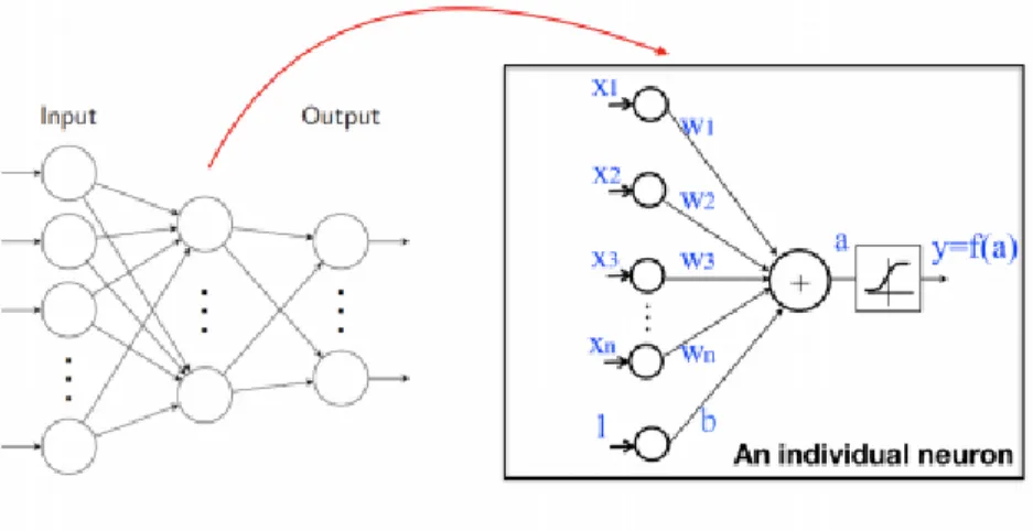
Figure 1-3: The schematic of fully-connected neural networks. This figure is adopted from the MIT 6.869 (taught by Prof. Bill Freeman and Prof. Antonio Torralba).

Figure 1-4: Multi-layer convolutional neural network: generic scheme. Figure reprinted from [1] with permission.

will introduce later that adopted the idea of parameter sharing, the primary machine learning architecture to tackle image-related problems. Thanks to parameter sharing, CNNs are able to dramatically lower the number of unique parameters and to signif-icantly increase network sizes without having to correspondingly increase number of training data.

1.2.2

Convolutional neural networks and their applications in

computational imaging

Natural images have many statistical properties that are invariant to translation and CNNs take into account this property by sharing trainable parameters across multiple image locations. CNN, as the name suggests, employs the linear operation convolution to replace the general matrix multiplication in its layers. As Fig. 1-5 shows (1D simplification), if the kernel is of size 𝑁 × 1, neuron 𝑖 at layer 𝑙 is connected to the 2𝑁 + 1 nearby neurons from the previous layer, namely,

𝑎𝑖 = 𝑁

∑︁

𝑛=−𝑁

𝑤𝑛𝑥𝑖−𝑛+ 𝑏𝑖, (1.17)

where the trainable weights 𝑤𝑖’s are shared across the image. In the actual image,

then the input would be the weighted sum of the outputs of the neighbouring (2𝑀 + 1) × (2𝑁 + 1) neurons from the previous layer, where 𝑀 × 𝑁 is the kernel size. Afterwards, non-linearity activation functions are applied, as mentioned in the last subsection.

Figure 1-5: Convolutional neural networks. This figure is adopted from [2] with permission.

Convolution operation leverages three key ideas that can help improve a machine learning system: sparse representation, parameter sharing and equivariant represen-tation [31]. Sparse represenrepresen-tation refers to the sparse connectivity between neurons

in adjacent layers, significantly reducing the number of operations needed in the neu-ral network. This is practically possible as the useful features are typically much smaller than the size of images. Parameter sharing, as we stated before, each mem-ber of the kernel is used at every position of the input, with the exception of some boundary values. It is possible since many useful features are universal across the images and by parameter sharing, the storage requirement for parameters is greatly reduced. Finally, the particular form of parameter sharing causes the layer to have the equivariance to translation. This is particularly useful since often times there are some functions of small number of neighbouring pixels are useful when applied to multiple input locations. See [31] or other textbooks on deep learning for a more detailed introduction on deep CNNs.

Worth special noting is that many modern deep convolutional neural networks assume one of several classical architectures, including U-Net [53], Residual Neural Networks (ResNet) [54] and Densely Connected Neural Networks (a.k.a DenseNet) [55].

Deep learning has been applied to almost of all representative applications in computational imaging, including [5, 56, 57] for quantitative phase retrieval, [58, 59] for imaging through the scattering medium, [4,60–63] for image super-resolution, and numerous others. See [1] for an extensive review. A commonality of many of these works, however, is that DNNs are typically trained in an End-to-End, supervised fashion, where the system physics is not explicitly leveraged, making the training a “black-box" and therefore lacks interpretability. Moreover, when the problem is in the most ill-posed conditions, e.g. the noise is strong, the DNN carrying not only the burden of learning the system physics as well as the regularizer, jeopardizing the DNN performance. Instead, in many cases, we do have good knowledge about the forward model and therefore the intuition is that physics-informed DNN algorithms will be more efficient and introduce breakthrough to the performance of DNN algorithms.

1.3

Thesis outline

The outline of the remainder of the thesis is as follows:

In Chapter 2, we introduced the learning-to-synthesize by DNN (LS-DNN), a deep learning framework where the power-spectral prior of the training examples motivated us split, process and recombine low and high frequency bands, to achieve full-band reconstructions with high fidelity, combating the common limitation of most deep learning algorithms where loss of high frequencies generally occurs in the recon-structions. We found the cause of such limitation is two-fold: on one hand, most physics operators suppress high frequencies, which requires the algorithm to learn to compensate high frequencies from the training data; what makes things worse, the under-representation of high frequencies in the training examples make it increasingly more difficult for the high frequencies to survive the highly non-linear training process according to their fair share.

To tackle this difficulty, we propose a two-step process, where in the first step, two DNNs are trained in parallel, with unfiltered and filtered ground truth examples where the power-spectral density of the examples are altered to emphasize the high frequencies; at the end of the first step, preliminary reconstructions are produced by the pair of DNNs, with the anticipation that the each is reliable in low and high frequency band, respectively. Subsequently, we propose to use a third DNN to learn to synthesize the preliminary reconstructions, or equivalently, the high and low frequency bands, to achieve the final reconstructions that is of high fidelity in all frequency bands. We demonstrate the LS-DNN scheme using standard computational imaging applications, including image super-resolution, phase retrieval both under ample light conditions and under low light conditions. Reconstructions show that the LS-scheme is crucial for better image reconstruction quality, especially under the most ill-posed conditions. What is worth special mentioning is that the LS scheme demonstrated desirable robustness to noise, which opens its door to other computational imaging applications under noisy conditions.

Network (PLT-PhENN) to solve phase retrieval at low photon counts and addressed the deficiency of high frequencies in the reconstructions in [64]. The crux of PLT-PhENN is that, PLT-PhENN is trained not to match the reconstructions with the ground truth in the image domain, but instead on the feature maps extracted from a pre-trained DNN on a separate image-classification problem. Perceptual loss trained image-transformation DNNs have not been used in phase retrieval, or any problem under severe noise. We discovered that the grid-like artifacts, pronounced only un-der strong noise, display a clear periodicity, with the fundamental frequency halved by each encounter of MaxPooling2D layer in VGG. We therefore modify the previous common practice to instead train the DNN by feature maps at ReLU-12, which lead to reconstructions significantly better than [64], both visually and quantitatively. More importantly, this modification of the rule of thumb of training perceptual loss trained image-transformation DNNs should invite future investigations into many computa-tional imaging problems under noisy conditions that rely on machine learning.

In Chapter 4, we answered two fundamental yet related unanswered questions in using deep learning in computational imaging, First, whether models trained on one class of examples directly generalize well to a disjoint class. In practice, seldom does one enjoy the luxury of having large scale annotated training examples in the intended class. This is especially true if the data need to be acquired experimentally and also if we work in some certain domains, e.g. biological samples. One possible compromise is to train the deep learning architecture using the publicly available standardized datasets. After the model is trained, it is used to reconstruct examples in the intended class. Thus, for example, it would be possible to train using natural images and then use the model to image biological cells. If we are to do such a thing, we need strong reassurance that the learned priors work correctly, or the cell images could not be trusted. And second, whether the trained neural network has learned the underlying physics model, and it pertains to the interpretability of deep learning algorithms. We found these two questions to be directly related, due to the following argument: if the trained DNN has learned the physical model well, then this property should be beneficial for cross-domain generalization performance as well.

Moreover, we find that the common essence is the training examples used — if the DNN is trained with more generic datasets, e.g. ImageNet, then it will be guided to learn the underlying physics model better and this leads to better cross-domain generalization performance; conversely, if it is trained with more restricted datasets, e.g., MNIST, then the overly strong regularization effect imposed by the MNIST training examples encourages the DNN to minimize the training loss by learning to produce examples similar to the training examples, instead of capturing the physics model, and that causes the cross-domain generalization to become problematic. The generic/restrictive behavior of a dataset is quantified by the Shannon entropy of the dataset contents, with the rationale that higher entropy corresponds to higher level of uncertainty of the pixel-values, making the class more generic. Conversely, lower entropy implies lower uncertainty and a more restrictive class. This choice of met-ric provides the readers an easy guideline for choosing the appropriate standardized training dataset for better cross-domain generalization ability.

In Chapter 5, we propose to use deep learning to enable fast, real-time optical diffraction tomography (ODT) from a single-shot angle-multiplexing interferogram. In ODT, we typically reconstruct the 3D refractive index map from multiple 2D pro-jections (holograms or intensity measurements) obtained from different illumination angles. Traditional ODT algorithms suffer from the bottleneck of imaging speed, due to the iterative nature of the computational algorithms. Moreover, the need to cap-ture projections from each individual angle make the data-acquisition time longer, introducing motion blur and instability due to the mobility of the living biological cells. To improve over these issues, we propose to use single-shot angle-multiplexed in-tereferogram based on limited number of angles, which is formed by turning on limited number of illumination at various angles simultaneously and base the reconstruction algorithm solely on this single-shot interferogram. Deep learning is introduced to enhance the reconstruction speed. Various deep learning based strategies to achieve this ultimate goal are proposed and the common gist is that only a small number of individual phase maps extracted from the individual interferograms are sufficient, thanks to machine learning that allows us to compensate the missing information

from data, to provide us good final 3D RI maps. Significant progresses that have been made toward this ultimate goal will be reported.

In Chapter 6, we propose the cascaded neural network architecture for compu-tational inverse problems. The cascaded network, which rests upon the proximal gradient descent algorithm, allows the physics operator to be directly incorporated into the learning process. The neural network to learn to function as the ideal Prox-imal operator from the data (thus termed “learning to regularize"), as the ProxProx-imal operator is a function of the regularizer used and thus the appropriate underlying regularization has been learned indirectly. In this Chapter, we use low-light phase retrieval as the representative application and show that the incorporating the physics into the DNN does outperform the end-to-end scheme [56] and performs similarly to the physics-informed scheme [64]. Moreover, we propose as future works, the other framework of algorithm unrolling for blind deconvolution under low light conditions based on a class of neural networks based on a generative model for convolutional dic-tionary learning (CDL) using data from the natural exponential-family, e.g. Poisson distribution.

In Chapter 7, we conclude the thesis and point out directions for ongoing and future investigations.

Chapter 2

Learning to synthesize: splitting and

recombining low and high spatial

frequencies for full-band image

recovery

2.1

Motivation

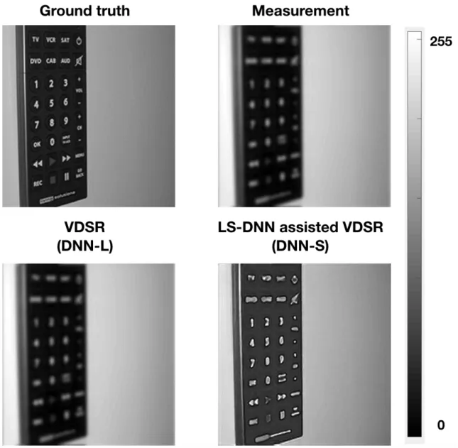
As mentioned in the last Chapter, deep learning (DL) has been proven successful in many applications of computational imaging. However, the reconstructions by the existing deep-learning algorithm usually present an uneven fidelity in low and high frequencies — the reconstructions are usually quite accurate in the low frequency band but is not accurate in the high frequency band, manifested by the oversmooth-ness in the reconstructions. For example, Fig. 2-11 showed the results for image super-resolution by the very deep neural network for super-resolution (VDSR) [65], a benchmark deep learning architecture for image super-resolution for the images, we see the digits on the controller cannot be clearly seen from the VDSR reconstruction, without the LS-DNN scheme that we will propose in this Chapter, being applied.

First, many forward operators suppress high frequencies. In Fig. 2-1 diffraction-limited imaging, a representative linear inverse problem, due to the finite aperture of the imaging system, presents a hard cut-off of high frequencies. Moreover, in phase retrieval, a non-linear inverse problem of particular interest, the forward operator scrambles high frequencies. Therefore, the DNN has to rely on the prior information presented to the training.

Figure 2-1: Effect of forward operators in the frequency domain. (a) an ImageNet example. (b) diffraction-limited measurement, (c) and (d) are the Fourier spectrum of (a) and (b), respectively. (e) A sinusoidal phase object. (f) Intensity measurement, (g) and (h) are 1D cross-sections along the horizontal direction for the Fourier spectrum of (e) and (h), respectively.

Second, however, for most examples of practical interest, high frequencies are more sparse than the low frequencies, though they do play an important role in the quality of the images as they carry important information about the fine textures of the ob-jects. For example, in Fig. 2-2 the natural images have an inverse-square power law (spatial) power-spectral density (PSD), i.e., 𝑆(𝑢, 𝑣) = (√𝑢2 _{+ 𝑣}2₎−2 _{[66]. However,}

this very sparsity makes it increasingly more difficult for the high frequencies to sur-vive the highly non-linear training process and results in high frequencies presenting in the reconstructions for less than their fair share.

Figure 2-2: Log-log scale of power-spectral density of natural images.

2.2

Preliminary work— DNNs trained with

exam-ples with spectral pre-modulation

To combat this issue, [3] attempted to train the phase extraction neural network (PhENN) [56] instead with the pre-filtered examples and their corresponding inten-sity measurements. The authors propose to pre-filter the examples with spectral filter 𝑇 (𝑢, 𝑣; 𝜃) = (√𝑢2_{+ 𝑣}2₎𝜃 _{such that ˜𝐹 (𝑢, 𝑣), the Fourier transform of the filtered}

example ˜𝑓 , and 𝐹 (𝑢, 𝑣), the Fourier transform of the original example 𝑓 , satisfies, ˜

𝐹 (𝑢, 𝑣) = 𝐹 (𝑢, 𝑣)𝑇 (𝑢, 𝑣). In this paper, the authors propose to flatten the PSD of the filtered examples by using 𝑇 (𝑢, 𝑣) = √𝑢2_{+ 𝑣}2 _{or 𝜃 = 1. During the test stage,}

unfiltered measurements were used as the input to the PhENN to produce the re-constructions. Fig. 2-3 shows an example of the original and pre-filtered examples and their respective Fourier spectrum. The flowchart of the scheme is provided in

Fig. 2-4.

Figure 2-3: Spectral pre-modulation. (a). Original image 𝑓 in ImageNet. (b). The spectrally pre-filtered image ˜𝑓 . (c). Fourier transform of original image 𝐹 (𝑢, 𝑣). (d). Fourier transform of the spectrally pre-filtered image ˜𝐹 (𝑢, 𝑣). Figure reproduced from [3] with permission.

The rationale of this scheme is that although PhENN is trained to learn the same underlying physical model, namely, the (inverse) free-space propagation, the pre-filtered training examples implant the prior information to the DNN that the reconstructed examples should contain more high-frequency components than those produced with canonically-trained PhENN. Therefore, the resolution of the recon-structions is expected to improve, however, as this frequency pre-filtering intention-ally violated the prior of the desired examples (the examples we want to produce are not subject to the same pre-filtering), therefore distortions in the reconstructions are also to be expected.

Figure 2-4: The flowchart of PhENN trained with spectrally pre-filtered examples. (a). the training stage. (b). the test stage.

examples can only resolve dots that are at least 𝐷 = 6 pixels apart, according to the Rayleigh resolution test; however, PhENN trained spectral pre-filtered examples can resolve pixels that are 𝐷 = 3 pixels apart. Thus, the spatial resolution is improved by a factor of two, thanks to the spectral pre-modulation.

However, as discussed before, the enhanced resolution does not lead to better reconstructions. In Fig. 2-7, we see that the estimated phase objects produced by the original PhENN is quite accurate in the low-frequency band but not in the high-frequency band; on the other hand, those produced with PhENN trained with spec-trally pre-filtered examples are much better in the fine details, at the cost of the visible high-frequency artifacts and low-frequency distortions. Therefore, this scheme is not good enough for our ultimate goal: full-band high-quality phase imaging.

Figure 2-5: Resolution of the original PhENN.(a) dot pattern example for the resolu-tion test. (b) PhENN reconstrucresolu-tions for dot pattern with D = 2 pixels. (c) PhENN reconstructions for dot pattern with D = 3 pixels. (d) PhENN reconstructions for dot pattern with D = 6 pixels. (e) 1D cross-sections along the lines indicated by red arrows in (b)-(d). Figure reproduced from [3] with permission.

2.3

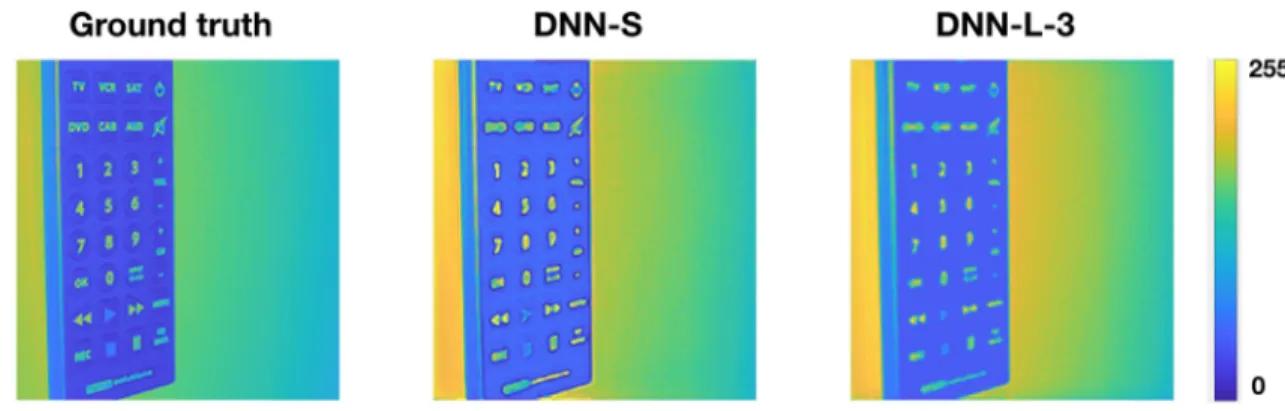
Methodology of learning to synthesize by DNN

(LS-DNN)

Despite the reconstructions by the spectral pre-filtering PhENN being unsuccessful, this line of thoughts inspired the learning to synthesize scheme (LS), the central topic for this chapter, which allows reconstructions with high-fidelity in all frequency bands. The study indicates that the LS-scheme is effective to many applications of computational imaging, especially in the most ill-posed case, i.e., imaging under low-light condition.

Figure 2-6: Enhanced resolution of PhENN by the spectral pre-modulation. (a) dot pattern example for the resolution test. (b) PhENN reconstructions for dot pattern with D = 2 pixels. (c) PhENN reconstructions for dot pattern with D = 3 pixels. (d) PhENN reconstructions for dot pattern with D = 6 pixels. (e) 1D cross-sections along the lines indicated by red arrows in (b)-(d). Figure reproduced from [3] with permission.

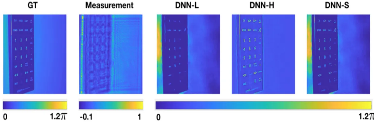
two separate DNNs, namely the low-frequency DNN (DNN-L) and the high-frequency DNN (DNN-H) are used to split and process low and high frequencies and obtain reconstructions reliable in the respective frequency bands. Subsequently, we used a synthesizer DNN (DNN-S) to learn to synthesize the preliminary reconstructions into the final reconstruction that is reliable in the full band.

In Fig. 2-8, we show the two-training steps of LS-DNN. The first step consists training two separate DNNs in parallel, as follows:

∙ DNN-L is trained to match the unfiltered patterns 𝜉(𝑛)_{(𝑥, 𝑦) at its input with the}

corresponding unfiltered example phase patterns 𝑓(𝑛)_{(𝑥, 𝑦) as ground truth at}

Figure 2-7: Reconstructions with ordinary and spectrally pre-modulated PhENN. (a) ground truth for a phase object. (b). diffraction pattern captured by the CMOS (after background subtraction and normalization). (c). phase reconstruction by PhENN trained with original ImageNet examples. (d). phase reconstruction by PhENN trained with spectral pre-modulated examples. Figure reproduced from [3] with permission.

intensity measurement in the End-to-End scheme [56, 62]; or the Approximant, in the Approximant approach [5, 57]].

∙ DNN-H is trained to match the unfiltered patterns 𝜉(𝑛)_{(𝑥, 𝑦) at its input to}

corresponding spectrally filtered versions 𝑓𝑝(𝑛)(𝑥, 𝑦) of the ground truth examples

𝑓(𝑛)(𝑥, 𝑦) at its output.

The output of DNN-L for a general test input 𝜉(𝑥, 𝑦) is denoted as ˆ𝑓LF(𝑥, 𝑦). Assuming similar training conditions, ˆ𝑓LF_{matches the output of PhENN as presented}

expected to be fairly accurate at low spatial frequencies but missing fine details. The output of DNN-H is denoted as ˆ𝑓HF_{(𝑥, 𝑦). Note that [3] required spatial}

pre-filtering the raw inputs 𝑔; here, we do not spatially pre-filter the input 𝜉 (i.e., 𝑔 or ˆ𝑓* according to whether the End-to-End or Approximant scheme is used). We instead train DNN-H to produce the filtered output based on an unfiltered input. This leads to better generalization, because DNN-H is trained on the broadest set of possible images (whereas the training in [3] was on high-frequency containing images only). Moreover, using unfiltered inputs to DNN-H allows for the training process to be parallelized for better efficiency.

Depending on the value of the power law 𝑞, the PSD of the patterns training DNN-H will be flat or almost flat. The output of DNN-H ˆ𝑓HF_{(𝑥, 𝑦) is expected to}

have better fidelity at fine spatial features of the phase objects. However, spectral flattening may also generate artifacts due to over-learning the high spatial frequencies. Therefore, ˆ𝑓HFlooks rather like a high-pass filtered version of the true object 𝑓 , which we found to be more beneficial for subsequent use in the LS scheme.

The second training step consists of combining the two partially accurate recon-structions ˆ𝑓LF _{and ˆ𝑓}HF _{into a final estimate ˆ𝑓 (𝑥, 𝑦) with uniform quality at all spatial}

frequencies, low and high up to the passband. To this end, we train the synthesizer DNN-S to receive ˆ𝑓LF _{and ˆ𝑓}HF _{as inputs, and use the un-filtered examples 𝑓 as the}

output. To avoid any further damage to the high-spatial frequency content in ˆ𝑓HF, we bypass ˆ𝑓HF _{and present it intact to the last layer of DNN-S. By operating on}

ˆ

𝑓LF alone, DNN-S learns how to treat the low frequency reconstruction so as to com-pensate for artifacts at all bands. The use of the synthesizer DNN-S also makes our results less sensitive to the choice of power 𝑞. We found that 𝑞 ∈ [0.3, 0.7] can produce reconstructions of approximately even quality, as presented in Section 2 of [57].

After DNN-L, DNN-H and DNN-S have been trained, they are combined in the LS system and operated as shown in Figure 2-8(b). The input 𝜉(𝑥, 𝑦) is passed to DNN-L and DNN-H in parallel fashion, and the respective outputs ˆ𝑓LF(𝑥, 𝑦) and ˆ𝑓HF(𝑥, 𝑦) are passed to DNN-S, which produces the final estimate ˆ𝑓 (𝑥, 𝑦). It is worth noting that it is not valid to lump the three networks in Figure 2-8(b) into a single network,

updating weights Residual U-Net updating weights

(a)

+

(b)

Figure 2-8: Scheme for LS-DNN. (a). training stage (b). test stage.

due to their separate training schemes described above.

one particular possibility is to instead using the low-pass filtered examples, which was the case adopted in the DualCNN scheme [4], which we will compare with the LS scheme in Section 2.4.1; One great advantage of the current LS scheme is so that it can quickly pair up and improve over the existing state-of-art scheme, by making the existing state-of-the art DNN as DNN-L. Such vast improvement will be demonstrated later in Fig. 2-11.

The validity of the methodology does not seem to rely on the any specific appli-cations, as long as the underlying forward operator suppresses high frequencies; and, the database of interest are over-represented by low spatial frequencies, both of which are commonplace in practice. In this thesis, we conduct the investigations with two representative inverse problems in computational imaging, i.e., super-resolution in diffraction-limited imaging and quantitative phase retrieval. For phase retrieval, we showed results both under low noise and high noise conditions.

2.4

Results

2.4.1

Low-noise image super-resolution in diffraction-limited

imaging under incoherent illumination

Image super-resolution is a central topic in computational imaging and computer vision. However, they have different interpretations in different research communities. In computer vision community, it usually means upsampling, i.e. from the raw image 𝑔 with limited number of pixels to arrive at the estimate ˆ𝑓 that have more pixels within the same spatial support; it can also be interpreted as deblurring, where the blur kernel is a low-pass filtering with transfer function equal to zero for spatial frequencies above the cut-off frequencies [67].

There are thousands of previous works of image super-resolution under the up-sampling interpretation using non-machine learning methods. Please refer to [68] for an extensive review. To our knowledge, [60,61] are the first works using deep learning in the upsampling context and [9,69] are among the most important follow-ups where