A decomposition approach for commodity pickup and delivery with time-windows under uncertainty

A decomposition approach for commodity pickup

and delivery with time-windows under uncertainty

The MIT Faculty has made this article openly available.

Please share

how this access benefits you. Your story matters.

Citation

Marla, Lavanya, Cynthia Barnhart, and Varun Biyani. “A

Decomposition Approach for Commodity Pickup and Delivery with

Time-Windows Under Uncertainty.” Journal of Scheduling (February

15, 2013).

As Published

http://dx.doi.org/10.1007/s10951-013-0317-1

Publisher

Springer-Verlag

Version

Author's final manuscript

Citable link

http://hdl.handle.net/1721.1/89058

Terms of Use

Creative Commons Attribution-Noncommercial-Share Alike

Detailed Terms

http://creativecommons.org/licenses/by-nc-sa/4.0/

(will be inserted by the editor)

A Decomposition Approach for Commodity Pickup and

Delivery with Time-Windows Under Uncertainty

Lavanya Marla · Cynthia Barnhart · Varun Biyani

Received: date / Accepted: date

Abstract We consider a special class of large-scale,

network-based, resource allocation problems under un-certainty, namely that of multi-commodity flows with time-windows under uncertainty. In this class, we fo-cus on problems involving commodity pickup and de-livery with time windows. Our work examines meth-ods of proactive planning, that is, robust plan genera-tion to protect against future uncertainty. By a priori modeling uncertainties in data corresponding to service times, resource availability, supplies and demands, we generate solutions that are more robust operationally, that is, more likely to be executed or easier to repair when disrupted. We propose a novel modeling and solu-tion framework involving a decomposisolu-tion scheme that separates problems into a routing master problem and scheduling sub-problems; and iterates to find the opti-mal solution. Uncertainty is captured in part by the master problem and in part by the scheduling sub-problem. We present proof-of-concept for our approach using real data involving routing and scheduling for a large shipment carrier’s ground network, and demon-strate the improved robustness of solutions from our approach.

Lavanya Marla

iLab, Heinz College, Carnegie Mellon University Pittsburgh, PA.

E-mail: lavanyamarla@cmu.edu Cynthia Barnhart

Department of Civil and Environmental Engineering, Mas-sachusetts Institute of Technology

Cambridge, MA.

E-mail: cbarnhart@mit.edu Varun Biyani

Heinz College, Carnegie Mellon University Pittsburgh, PA.

E-mail: vbiyani@andrew.cmu.edu

Keywords robust routing and scheduling ·

multi-commodity routing and scheduling · uncertainty · decomposition

1 Introduction

In this paper, we consider the class of large-scale network-based problems including multi-commodity flow lems with time-windows, which are at the core of prob-lems arising in transportation, communications and lo-gistics. Such resource allocation problems with their large-scale nature and associated complexity, have been ideal candidates for the application of optimization tech-niques (Barnhart et al. 1994; Desrosiers et al. 1995; Barnhart et al. 1998a; Dumas et al. 1991). However, conventional optimization techniques usually involve as-sumptions of deterministic inputs, leading to solutions that are easily disrupted when realized parameter val-ues are different; and thus exhibit a lack of robustness and high costs of recovery or repair. Such solutions are rarely (if ever) executed, and certainly, never truly op-timal. In this work, our objective is to build robust network resource allocation solutions that: (i) are less fragile to disruption, (ii) easier to repair if needed, and (iii) minimize the realized, not just planned, problem costs.

Uncertainty in multi-commodity flows with time-windows can occur in the form of stochasticity in the supplies and demands of commodities; available capac-ities of the network links; and travel and service times on the network. The multi-commodity flows with time-windows is at the core of network design problems, and hence, in finding robust solutions to the multi-commodity flows with time-windows we expect to

pro-vide insights into the more complex problem of network design under uncertainty.

1.1 Problem Description

To illustrate and evaluate our approach, we consider a specific problem, namely the Commodity Routing

Prob-lem with Time Windows Under Uncertainty (CRTW-UU ). Under CRTW-(CRTW-UU, for each vehicle v (such as a

plane or truck) in the set of vehicles V , we are given a set of vehicle routes defining a network of locations with time-independent travel times and capacities uij

corresponding to vehicle capacities on the links, and service times at locations. Each commodity k (such as a trailer, package, crew member or passenger) in the set of commodities K with demand dk needs to be routed

over this network, from its origin O(k) to its destination

D(k). Transshipment routing is allowed. All dkunits of

commodity k are assumed to have the same route and schedule. (In cases where different units of a commod-ity can have different routes and schedules, each unit can be treated as a commodity by creating dk

sepa-rate commodities. Thus this assumption has no loss of generality.) Commodity k must be picked up after its earliest available time at its origin (EATk

O(k)) and

de-livered before its latest delivery time at its destination (LDTk

D(k)). The objective is to find commodity routes,

and vehicle and commodity schedules, which minimize costs due to vehicle operations, and non-service of com-modities. We consider early drop-offs to have no bonuses, and we disallow late drop-offs (that is, if a commodity is late, it will not be delivered). We are therefore inter-ested in determining commodity routes and commodity and vehicle schedules, given the sequence of stops each vehicle makes. In this work, we are particularly inter-ested in addressing the stochastic nature of input data as seen in vehicle capacities, demands of commodities, and service times. In the remainder of the paper, we use the words ‘commodity’, ‘shipment’ and ‘trailer’ in-terchangeably.

CRTW-UU is at the core of the classic network de-sign problem of vehicle routing with pickup and deliv-ery of shipments under time-windows and under

uncer-tainty (Cordeau et al. 2006). The problem of vehicle

routing with pickup and delivery of shipments under time-windows under uncertainty reduces to the CRTW-UU if we assume the routes of vehicles to be known, with the schedule still unspecified. Instances (and vari-ants) of the CRTW-UU arise in package delivery, con-tainer scheduling, airline scheduling, etc. These prob-lems have been shown to be NP-hard Cordeau et al. (2006), and are more so in the case of uncertainty.

Approaches to capture uncertainty and build robust solutions have been in three categories: (i) tailored ap-proaches, (ii) general, distribution-free apap-proaches, and (iii) general-distribution-based approaches. Tailored ap-proaches like Shebalov and Klabjan (2004), Lan et al. (2006), Paraskevopoulos et al. (1991) and Kang and Clarke (2002) identify specific features of the problem that can make the solution flexible, and maximize such attributes. General, distribution free approaches do not capture distribution information, but use information about uncertainty sets, as described in Soyster (1973), Ben-Tal and Nemirovski (1999), Ben-Tal and Nemirovski (2000), Bertsimas and Sim (2004) and Bertsimas and Sim (2003). General, distribution-based approaches such as Birge and Louveaux (1997), Charnes and Cooper (1959), Charnes and Cooper (1963), Rockafellar and Uryasev (2000) and Mulvey et al. (1981) model the un-derlying distributions analytically or through scenarios, to generate robust solutions for those distributions. In this work, our goal is to develop analytical and com-putational frameworks that help us take advantage of partial knowledge of data distributions, for example, in the form of quantiles.

Other studies have modeled uncertainty in the vehi-cle routing and multi-commodity flow contexts. Bertsi-mas and Simchi-Levi (1996) survey the vehicle routing problem (VRP) literature and studies the determinis-tic, dynamic and stochastic variants for the VRP. In the stochastic and dynamic cases, they study uncer-tainty in demands, location or arrival time of requests. For these, in particular, for the dynamic version, good solutions can be found by adapting the static meth-ods appropriately. For stochastic VRPs, they consider the VRP under congestion, and based on structural in-sights from these problems, construct algorithms for the stochastic and dynamic cases. However, commod-ity pickup and delivery under uncertainty is not con-sidered. Dror et al. (1989) study the vehicle routing with stochastic demands. They propose two new solu-tion frameworks - one is a stochastic programming with recourse model that can be applied for structures with relatively general recourse actions, and the second is a Markov decision process based model. The authors do not consider uncertainty in other elements of the problem, and do not provide computational proof-of-concept. Mahr (2011) studies the problem of truckload pickup-delivery-and-return problem with time-windows, with release time-uncertainty, truck breakdown uncer-tainty and service time unceruncer-tainty. The author pro-poses a substitution algorithm that improves the per-formance of the agent-based approach in cases with and without uncertainty. He also shows that distributed heuristics are comparable to centralized optimization

methods in the case of dynamic pickup and delivery problems. Yang et al. (2004) consider a real-time (dy-namic) multi-vehicle pickup and delivery problem, where requests arrive in real time, and their pickup and deliv-ery windows are known at arrival. They propose formu-lations for the offline and online contexts of the prob-lem, and describe that the best policy is one that takes some future demand distribution into consideration. This points to the necessity of robust models, although the paper does not explicitly plan for robustness.

Dessouky et al. (1999) study the impact of man-aging uncertainty by increasing the amount of infor-mation available, in the context of bus dispatching. They use technologies that enable greater control of systems by tracking information in real-time and using the information to control schedules, thus improving service levels. However, they consider in this paper an information-sparse scenario without implementation of intelligent transportation systems. Sungur et al. (2010) consider the courier delivery problem with probabilistic customer arrivals and uncertain travel times, and use an approach that combines stochastic programming with recourse to model customer arrival uncertainty and ro-bust optimization to capture uncertainty in travel times. This scenario-based approach maximizes customer cov-erage and route similarity over scenarios, and minimizes earliness and lateness penalties and total travel times. This is a network design problem unlike the CRTW-UU. For large-scale problem instances, therefore, the authors use insertion-based heuristics to balance the multiple objectives presented. Wollmer (1980) consid-ers multi-commodity flow networks where link capac-ities are uncertain and commodcapac-ities are to be trans-ported from origin to destination. The objective is to find an investment strategy that adds link capacities while minimizing associated expected investment costs for increasing link capacities. A two-stage stochastic program is formulated, wherein the objective of the sec-ond stage is to minimize transportation costs once link capacities are realized. This is again a network design problem, solved using stochastic optimization, which re-quires extensive scenario generation and knowledge of distributions of uncertain parameters to solve the prob-lem. Ordonez and Zhao (2011) solve a similar problem by applying a robust optimization framework to the problem of expanding network capacity when demand and travel times are uncertain. This work is a network design problem, but is closest to our work in the goal of capturing both demand and travel time uncertainty in the presence of partial information about uncertainty.

1.2 Motivation for a new approach

While there has been extensive work on capturing spe-cific types of uncertainty (such as demand uncertainty or travel time uncertainty) separately, there is relatively less work (for example, Sungur et al. (2010) and Or-donez and Zhao (2011)) on capturing both types of uncertainty and generating robust solutions. Moreover, most models require knowledge of uncertainty distri-butions, whereas in practice, data generated from the field has only partial knowledge of the underlying dis-tribution. Our goal is to develop a framework for the CRTW-UU that helps capture multiple kinds of uncer-tainty simultaneously, while having the ability to make use of data distributions, if known, or partial informa-tion, if available (for example, in the form of quantiles).

1.3 Contributions

In addressing the CRTW-UU problem, our contribu-tions are as follows. First, to capture demand and ca-pacity uncertainty, we extend the Chance-Constrained model of Charnes and Cooper Charnes and Cooper (1959) Charnes and Cooper (1963) and present our new Extended Chance-Constrained Programming (ECCP) model. Second, we develop a decomposition scheme that provides a new modeling and algorithmic approach, which captures travel time and demand uncertainty (building on the ECCP), and provides robust solutions that are less vulnerable to uncertainty. Our approach: (i) pro-vides a new way of modeling the problem by separat-ing the routseparat-ing and schedulseparat-ing elements of the problem, capturing different types of uncertainty in each, and maintaining accuracy by iterating among the modules; and (ii) is flexible with respect to data requirements in that it can be applied with partial or complete knowl-edge of data distributions.

1.4 Outline of the paper

In§2 we present our new decomposition modeling ap-proach. We present the different elements of the model and discuss how uncertainty is captured using this model. In§3 we present an algorithm to solve the decomposi-tion model. We then discuss the advantages and limi-tations of the approach. In §4 we apply our approach and discuss results for the problems of truckload rout-ing and schedulrout-ing for a U.S. carrier. We summarize and conclude in§6.

2 Decomposition Modeling Approach

2.1 Decomposition Overview

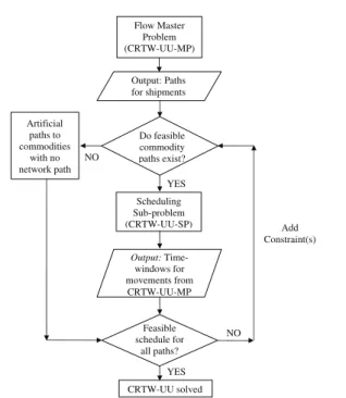
Our decomposition approach for CRTW-UU involves the repeated solution of a master problem and sub-problems. At each iteration of the procedure, the mas-ter problem is solved to generate a proposed solution to the CRTW-UU problem. The master chooses one path for each commodity from multiple paths available, while satisfying capacity constraints. The set of paths for each commodity include an ‘artificial’ path (a high cost path with zero travel time), which means a shipment cannot be delivered within the specified time windows and has to use a higher cost alternative. Each solution to the master problem ensures satisfaction of all constraints in the problem except scheduling constraints; and min-imum cost with respect to the satisfied constraints. To test if schedule infeasibilities exist in the solution, we solve sub-problems in which infeasibilities are detected using efficient network node-labeling algorithms. If no infeasibilities are found, a feasible schedule exists for the CRTW-UU solution and the CRTW-UU problem is solved. If, however, scheduling conflicts are identified, these scheduling conflicts are translated into inequali-ties that are added to the master problem to eliminate the current infeasible solution. After a finite (but pos-sibly large) number of iterations, our approach is guar-anteed to find a feasible, and hence optimal, solution to the CRTW-UU problem, as will be discussed in§3.6 and §3.7. A diagrammatic overview of our decomposi-tion approach is presented in Figure 1.

2.2 Flow Master Problem (CRTW-UU-MP)

When scheduling constraints are relaxed, the CRTW-UU reduces to flowing shipments on the vehicles. In solving it deterministically without modeling uncertainty, the flow master problem involves solving the standard path-based multi-commodity flow formulation detailed in Ahuja et al. Ahuja et al. (1993), that is, choosing paths for each commodity k on its subnetwork Gk.

To model uncertainty in demands and capacities, we extend the Chance-Constrained Programming (CCP) model (Charnes and Cooper 1959, 1963) of Charnes and Cooper and present our Extended Chance-Constrained

Programming model (ECCP). CCP is based on

con-straint satisfaction, that is, concon-straints containing un-certain capacity parameters are required to be satisfied for a pre-specified probability of protection γ. In our ECCP approach, however, the achieved level of protec-tion is modeled as a variable. We use partial informa-tion about the distribuinforma-tions of uncertain capacity

pa-Scheduling Sub-problem (CRTW-UU-SP) Feasible schedule for all paths? YES NO CRTW-UU solved YES NO Flow Master Problem (CRTW-UU-MP) Add Constraint(s) Do feasible commodity paths exist? Output: Paths for shipments Output: Time-windows for movements from CRTW-UU-MP Artificial paths to commodities with no network path ~

Fig. 1 Schematic diagram of the Decomposition Approach

rameters, in the form of quantiles; or full information in the form of distribution parameters. With each quan-tile is associated a level of protection, as defined by the Chance-Constrained Programming approach and defined more formally later in this section. Among these different levels of protection, our ECCP approach al-lows the model to maximize the level of protection un-der a robustness budget ∆. Compared to the Chance-Constrained Programming approach, the ECCP allows costs to be contained when achieving robustness and thus control the level of conservatism, and also avoids the necessity for the user to specify protection levels a

priori, which can be difficult when multiple uncertain

parameters in several constraints are involved Marla (2007). For further details of the approach, we refer the reader to Marla (2010). In the CRTW-UU, we capture uncertainty explicitly in capacities, that is, we protect against capacity drops. Through the increased slack in the capacity constraint, this acts as a proxy for protect-ing against demand uncertainty.

We now describe the network underlying the deter-ministic and ECCP models. For each shipment k we build a network Gk = (Nk, Ak) that is a copy of

net-work G = (N, A) described here. In G = (N, A), each node j∈ N has three attributes: a location l(j), vehicle

v(j) : v(j)∈ V , and information if it represents arrival

or departure of v at l(j). Connecting these nodes are arcs a∈ A of three types: travel arcs, connection arcs and transfer arcs. Travel arcs (i, j) on the network rep-resent movement of vehicle v(i)(= v(j)) departing from

l(i) and arriving at l(j). Flows on these arcs represent

the movement of shipments on v(i) from l(i) to l(j). Connection arcs connect the arrival node of v(i) at lo-cation l(i) and the departure node of v(i) = v(j) at

l(j) = l(i). Flows on these arcs represent shipments

re-maining on v(i) while it is positioned at l(i). Travel and connection arcs belong to Av, the set of arcs of vehicle v.

Flows on transfer arcs (i, j), which connect the arrival node of v(i) at l(i) to the departure node of v(j)(̸= v(i)) at l(j) = l(i), represent the transfer of shipments be-tween vehicles, and have an associated transfer time.

G = (N, A) is used to aggregate information (detailed

in §3) from the networks Gk= (Nk, Ak)∀k ∈ K. Each

arc (i, j)∈ G has a capacity of uij, that is determined

based on the type of arc (travel, transfer or connection arc). Pk _{is the set of origin to destination paths for}

commodity k in Gk. δijp is an arc-path indicator variable

that is equal to 1 if arc (i, j) is on path p, 0 otherwise. In addition, we have an artificial path for each ship-ment k ∈ K, which is not physically present in the shipment network Gk, but is used to model the case

when the shipment does not have any feasible path. The use of an artificial path in the solution denotes the schedule infeasibility of that shipment within the spec-ified time windows. cij is the cost on arc (i, j). cpis the

cost due to 1 unit of flow on path p, equivalent to the sum of costs of the arcs on the path. cp =

∑

(i,j)_∈p

cij.

Because we focus on finding feasible schedules, cij = 0,

and hence cp = 0 for all arcs and paths, except for

the artificial path (denoting schedule infeasibility). For each shipment k, the cost associated with the artificial path is a penalty cost (for no service or late service, or for subcontracting out the service to another carrier).

We summarize the notation for the model as follows:

– K = set of shipments k

– Gk = network for shipment k, constructed as de-scribed above.

– G = network that aggregates information from

net-works Gk,∀k ∈ K

– Pk _{= set of origin to destination paths for}

commod-ity k in Gk, including the ‘artificial’ path for k – dk = number of units of commodity k to be

trans-ported from origin to destination

– uij = capacity of arc(i, j)∈ G

– δ_ijp = arc-path indicator that is equal to 1 if arc (i, j) is on path p, 0 otherwise

– fp = 1 if all dk units of commodity k flow on any

path p∈ Pk; and 0 otherwise.

– cp = cost due to 1 unit of flow on path p (if p is the

artificial path this corresponds to penalties for no service, late service or subcontracting)

The deterministic formulation to find a path for each shipment on its subnetwork Gk, without capturing

any uncertainty, is the same as the path-based multi-commodity flow formulation, and is as follows:

min∑ k∈K ∑ p∈Pk dkcpfp (1) s.t. ∑ p∈Pk fp= 1 ∀ k ∈ K (2) ∑ k_∈K ∑ p∈Pk dkfpδpij≤ uij∀ (i, j) ∈ A (3) fp∈ {0, 1} ∀ p ∈ Pk,∀ k ∈ K (4)

The objective (1) minimizes costs of commodity flows on the network. Constraints (2) correspond to finding exactly one feasible path on the network for each com-modity, constraints (3) to ensure that flows satisfy arc capacity constraints, and constraints (4) correspond to integrality of commodity flows. We model the fp

vari-ables as binary because it is more advantageous when adding constraints from the Scheduling Sub-Problem into the Flow Master problem; and furthermore, make our approach easier to explain. This is without any loss of generality, as the dk units of each commodity k can

also be split into multiple commodities of one unit each. In order to capture uncertainty in demand or sup-plies (or, uncertainty in capacities as a proxy for demand uncertainty), we apply our ECCP model to (1) -(4). We first define the following additional notation.

– f_p′∗= optimal solution to the deterministic problem ((1) - (4)) that minimizes costs when data assume nominal values,

– uij= capacity of arc (i, j), indicating vehicle capac-ities or transshipment capaccapac-ities, depending on the type of arc,

– Qij = set of quantiles q = 1, ...|Qij| of uncertain

capacity parameters uij, for each constraint

corre-sponding to arc (i, j),

– uq_ij = capacity associated with quantile q∈ Qij, – pq_ij = protection level probability associated with

quantile q ∈ Qij for the capacity constraint

cor-responding to arc (i, j), 0 ≤ pq_ij ≤ 1; such that

P (uij ≤ uqij) = p q ij,

– yq_ij is the binary variable that is equal to 1 if the protection level expressed as a probability pq_ij, rep-resented by the qth quantile, is attained in the ca-pacity constraint for arc (i, j); and 0 otherwise,

– δ = pre-specified budget of cost from the nominal

value ∑ k∈K ∑ p∈Pk dkcpf ′_∗ p , and

– γij = achieved protection level for the capacity of arc (i, j).

The ECCP formulation corresponding to (1)-(4) is: CRTW-UU-MP: max ∑ (i,j)∈A wijγij (5) s.t.∑ k_∈K ∑ p_∈Pk dkcpfp≤ ∑ k_∈K ∑ p_∈Pk dkcpf ′_∗ p + ∆ (6) ∑ p_∈Pk fp= 1 ∀ k ∈ K (7) ∑ k∈K ∑ p_∈Pk dkfpδ p ij ≤ |Q∑ij| q=1 uq_ij(y_ijq − y_ijq−1)∀ (i, j) ∈ A (8) y_ijq ≥ y_ijq−1 ∀ q ∈ Qij,∀ (i, j) ∈ A (9) y_ij0 = 0 ∀ (i, j) ∈ A (10) y|Qij| ij = 1 ∀ (i, j) ∈ A (11) γij≤ |Q∑ij| q=1 pq_ij(yq_ij− y_ijq−1) ∀ (i, j) ∈ A (12) fp∈ {0, 1} ∀ p ∈ Pk,∀ k ∈ K (13) y_ijq ∈ {0, 1} ∀ q ∈ Qij,∀ (i, j) ∈ A (14) 0≤ γij ≤ 1 ∀ (i, j) ∈ A (15)

The goal of our model is to choose the solution with the highest level of protection, within a pre-specified budget δ.

(5) is the ECCP objective function that maximizes a weighted sum of protection levels (with weights wijand

achieved protection γij) over constraints with uncertain

parameters. Constraints (6) limit the expected cost of the robust solution to no more than a user-specified budget of ∆ more than the expected optimal cost when using nominal parameter values. Constraints (7) assign one path to each shipment. Constraints (8) find the highest protection level attainable for the uncertain pa-rameters. Inequalities (12) set γij to be no greater than

the highest protection level provided to the capacity constraint corresponding to (i, j). (9) ensure that the protection level variables follow a step function, that is, if a higher level of protection is achieved, all lower levels of protection are also achieved. (10) and (11) set the boundary values of the step functions. Constraints (13), (14) and (15) describe the variable ranges.

2.3 Scheduling Sub-Problem (CRTW-UU-SP)

Given a shipment flow solution F from the CRTW-UU-MP, the objective of the Scheduling Sub-Problem (CRTW-UU-SP) is to determine if the shipment flows

obtained from solving the Flow Master Problem have a feasible and robust schedule that obeys shipment pickup and delivery time-windows, allows connections and trans-fers, and has sufficient slack in its path. If a shipment is assigned to any path other than the artificial path in the solution to (5) - (15), it is possible that infeasibility might exist in its schedule. We determine the existence of a feasible robust schedule for the Flow Master Prob-lem solution by solving a series of shortest path and network-labeling algorithms, detailed in§3.1 and §3.3. If we find a feasible schedule, we are done, otherwise, the same algorithm identifies the sources of infeasibility. To find a robust schedule, we assign as a proxy a ‘protection level’ for each shipment path in the Flow Master Problem solution. The intuition behind this is that each shipment path is protected up to a certain probability level, the entire schedule is better protected because there is more flexibility in schedule movements. The higher protection basically adds slack in travel times by assuming higher quantiles of travel times (according to the protection level) than the average, thus adding buffers and allowing for movements under uncertain (and higher) travel time realizations. Note also that slack in the travel time also corresponds to wider time-windows of movements on the shipment path. The quan-tile value for the arc travel time to be used in the Scheduling Sub Problem can be determined based on the desired protection level for the path, using our knowl-edge of uncertainty based on historical data. Note that using this model, we protect only a subset of all arcs in the network, namely, those that are present on paths in the Flow Master Problem solution. This also helps avoid over-conservatism or ‘guessing’ in choosing which arcs to selectively protect, which would be the case in a non-decomposition based approach where path flows were not known before assigning protection levels to paths or arcs.

The protection level assigned to each arc in a ship-ment path needs to be chosen a priori by the user, and can be an iterative process. Our decomposition ap-proach also includes additional flexibility in changing the level of protection over iterations. The actual quan-tile of travel time used on an arc can be changed dur-ing the iterations of the decomposition approach. Dur-ing subsequent applications of the sub-problem to the master problem solution, higher quantile values may be used if a higher level of protection for the service times is desired.

2.4 Iterative Feedback Mechanism

We iterate between solving the CRTW-UU-MP and the UU-SP, identifying infeasibilities in the

CRTW-UU-SP solutions and adding them as new constraints into the CRTW-UU-MP in order to eliminate current infeasibilities. With each iteration, the constraints added to the CRTW-UU-MP increase its size minimally, but decrease the size of its feasible solution space. We will show that we converge to the optimal solution with each iteration of the algorithm. The CRTW-UU is solved when the shipment flows obtained from the CRTW-UU-MP have associated feasible schedules and no cuts are added, and the iterative procedure terminates.

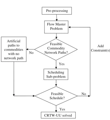
3 Solution algorithm for the decomposition modeling approach

In this section, we more formally describe the algo-rithm, depicted in Figure 2. As described in §2.2 and

§2.3, uncertainty is captured using the ECCP in the

Flow Master Problem and using quantiles for travel time using the CCP in the Scheduling Sub-Problem.

We improve the solvability of the Flow Master Prob-lem and Scheduling Sub-ProbProb-lem by invoking a pre-processing step that identifies time-infeasible path as-signments a priori. The Pre-processing step is executed before the commencement of iterations solving the Flow Master Problem and Scheduling Sub-Problem. We use the same notation introduced in §2, and detail each module of the Decomposition algorithm in the follow-ing sections.

3.1 Step 1: Network Pre-processing

On Gk, for all k∈ K, we define EATjk as the earliest

time shipment k can reach node j after starting from

O(k) and LDTk

j as the latest time shipment k can leave

node j to get to its destination D(k) on time. spk_i,jis the shortest path distance for shipment k from i to node j.

EATv

j and LDTjvare the earliest arrival time and latest

departure time of vehicle v at each node j∈ N. The steps of the network Pre-processing phase are detailed as follows:

(i) For each shipment network Gk for all k∈ K, based

on EAT_O(k)k and LDT_D(k)k , find time-windows, ex-pressed as the earliest arrival time and latest depar-ture time [EATk

i , LDTik], of any shipment k ∈ K

at each node i∈ Nk. Thus, EATik = EAT k O(k)+ sp k O(k),i; and (16) LDTik = LDTD(k)k − sp k j,D(k) (17)

(ii) Find time-windows (EATv

i, LDTiv) for each vehicle v∈ V at each node i ∈ N along its route based on

the earliest start time and latest allowed return time

Pre-processing Scheduling Sub-problem Feasible Schedule? Yes No CRTW-UU solved Yes No Artificial paths to commodities with no network path Flow Master Problem Add Constraint(s) Feasible Commodity Network Paths?

Fig. 2 Flow Chart of the Decomposition Approach

at the depot. These constraints are driven by driver work rules. If vehicle v does not pass through a node

i, i is labeled unreachable for v. For all reachable

arcs (i, j)∈ Av, for all v∈ V , we have

EAT_jv= EAT_iv+ ttij; and (18) LDT_iv= LDT_jv− ttij (19)

We label the time-windows and labels of vehicles and shipments thus obtained as pre-processing time

windows or labels. They are the broadest set of time

windows possible over any travel path for the vehi-cles and shipments (because these time-windows are formed using the shortest paths).

(iii) If LDTk

i − EATik < 0, the time-window duration of

a shipment k is negative at a node i∈ Nk. Because

the pre-processing time-windows are the broadest time-windows, no schedule feasible path for ship-ment k passes through i. For each shipship-ment network

Gk∀k ∈ K, remove all the schedule infeasible nodes,

and all arcs incident to these nodes. This results in a reduced version of Gk containing only those arcs

and nodes through which shipment k may pass. (iv) We say that the time-windows of shipment k and

vehicle v overlap at node i if the combined

vehicle-shipment pre-processing time-window has non-negative

duration. We denote the time-window at node i for the vehicle-shipment pair v and k as: (EAT_ik,v, LDT_ik,v), where EAT_ik,v= max{EAT_ik, EAT_iv} and LDT_ik,v=

min{LDT_ik, LDT_iv}. Find all possible overlaps of

shipment-vehicle pairs at each node i ∈ N, ∀ k ∈

K,∀ v ∈ V . If the overlap between time-windows

of shipment k and vehicle v is negative at node i, that is, LDT_ik,v− EAT_ik,v < 0, shipment k cannot

travel on the vehicle arcs in Av incident to node i. We delete such arcs and nodes from Gk, further

reducing its size. If the time-windows of a vehicle-shipment pair (v, k) are non-zero at both ends of an arc (i, j)∈ Av, shipment k can travel on (i, j), that

is, on that segment of vehicle v’s path, within the specified time-windows.

(v) Consider the aggregate network G with the vehicle-shipment pre-processing time-windows for all k∈ K superimposed on each other at each node i ∈ N. Suppose the time windows of two shipment-vehicle pairs (v, k1) and (v, k2) at a node i are individually

positive; but do not overlap with each other, thus making it infeasible for both k1 and k2 to travel

together on any (i, j)∈ Av in any schedule-feasible

solution to the CRTW-UU. This infeasibility can be eliminated from the set of feasible solutions to the Flow Master Problem by adding the following constraint to CRTW-UU-SP: ∑ p1∈Pk1|(i,j)∈p1 fp1+ ∑ p2∈Pk2|(i,j)∈p2 fp2 ≤ 1, (20)

where fp, p ∈ Pk is defined as in (5)-(15), that is,

it is a binary variable that takes on value 1 if ship-ment k is assigned to path p; and 0 otherwise. We add these constraints to the Flow Master Problem in the Pre-processing step to eliminate known infea-sible solutions.

3.2 Step 2: Flow Master Problem (CRTW-UU-MP)

The goal of the Flow Master Problem is to assign a route to each shipment in the network. We formulate the basic route choice without uncertainty as a multi-commodity flow problem of choosing paths on the net-works Gk (resulting after the Pre-processing step), for

each shipment in K. To capture uncertainty in capac-ities and demands, we use the Extended Chance Con-strained Programming (ECCP) Marla (2010) that re-sults in the CRTW-UU-MP. The ECCP maintains the structure of the multi-commodity flow problem and al-lows the use of implicit or explicit column generation techniques for large instances Marla (2007). (Column generation is a technique used in very large-scale for-mulations where variables number in millions or bil-lions, however only a subset of variables are included in the formulation to begin with. Implicit column genera-tion uses a mathematical formulagenera-tion to decide which

variables not already included should be brought into the Master Problem, without explicitly enumerating the variables. Explicit column generation on the other hand, enumerates the list of all (or most) variables and evaluates the value of adding them to the Master Prob-lem. Explicit column generation in very large-scale in-stances is often intractable, while implicit column gen-eration is efficient.) Other approaches that change the structure of the multi-commodity flow formulation, such as Bertsimas and Sim’s robust framework Bertsimas and Sim (2004) Bertsimas and Sim (2003), can also be used, and explicit column generation may have to be used for large-scale instances.

3.3 Step 3: Scheduling Sub-problem (CRTW-UU-SP)

After solving the CRTW-UU-MP, vehicle routes and assigned shipment paths p′₁, ..., p′_|K| for shipments k = 1, ...,|K| are known. Though the paths introduced into the Flow Master Problem are individually schedule-feasible, it is still possible that interactions between these shipment paths p′₁, ..., p′_|K|produce infeasible sched-ules. Therefore, in the Scheduling Sub-Problem, we ‘flow’ these shipments on the network G to determine a com-bined feasible schedule. Thus all the computations in this step are on the aggregate network.

When we wish to protect against travel time uncer-tainty, we do the following. Use an a priori chosen quan-tile (higher quanquan-tile) of travel time for all the shipment paths in the network. For all arcs belonging to shipment paths output by the Flow Master Problem in that

iter-ation, the travel time is selected to be a higher quantile

as described in§2.3. All other arcs in the network are assumed to have travel time equal to the mean travel time.

The Scheduling Sub-Problem consists of the follow-ing steps on the aggregate network:

i) Initialization: Let k = 0 represent the vehicle flows, and commodities k = 1, ...|K| represent the ship-ments.

(a) Set EATk

i = 0, and LDTik = M , a very large

number,∀i ∈ N, ∀k ∈ K. Set EATk

O(k)to EATk

at its origin, LDT_O(k)k = M , LDT_D(k)k to LDTk

at its destination, and EATk D(k)= 0.

(b) Set EATi= 0, and LDTi = M .

(c) Let Libe the label set at node i, consisting of the

list of shipments that impact the time-windows at i. Set Li= ϕ (empty).

(d) Set processing list to empty.

(e) For k = 0, 1, ...|K|, determine the time-windows for shipment k in sequence along its currently assigned path p′_k, (forwards from O(k) for EAT

values and backwards from D(k) for LDT val-ues) in the aggregate network, as indicated in (21) and (22).

EAT_jk= max{EAT_jk, EAT_ik+ ttij}

∀ (i, j) ∈ p′k,∀ k = 0, 1, ..., |K| (21) LDT_ik = min{LDT_ik, LDT_jk− ttij}

∀ (i, j) ∈ p′k,∀ k = 0, 1, ..., |K| (22)

These time-windows will at least be as tight as the Pre-processing step time-windows, because each shipment k ∈ K is restricted to path p′_k. The time-windows for the vehicles (k = 0) re-main the same as those in the Pre-processing step, because the vehicle routes are given inputs that do not change in solving the CRTW-UU. ii) For node i∈ N and k = 0, 1, ..., |K|,

(a) if EATk

i > EATi and EATik ̸= 0, set EATi = EATk

i, add k to Li if not already present.

(b) if LDT_ik < LDTi and LDTik ̸= M, set LDTi = LDTk

i, add k to Li if not already present.

(c) and add k to the processing list, if it is not al-ready present.

We refer to (EATi, LDTi) as the movement time windows at node i.

iii) For node i ∈ N if the movement time windows (EATi, LDTi) satisfy LDTi< EATi then there

ex-ist two shipments k1 and k2 in Li with paths p1

and p2 respectively passing through i, such that

EATk1

i > LDT k2

i .

(a) Without loss of generality, if k1 = 0 (it is a

ve-hicle path), add a constraint of the form

fp2 ≤ 0, (23)

(b) Else if k1> 0 and k2> 0 add a constraint of the

form:

fp1+ fp2 ≤ 1, (24)

to the Flow Master Problem.

iv) If the processing list is not empty, remove the first element from the list, add it at the end of the list, and go to step v.

v) Update EATi, LDTifor all (i, j)∈ p

′

k∀k ∈ 0, 1, ..., |K|,

(that is, for each arc in each vehicle path and each shipment path chosen by the Master Problem), pro-cessing (i, j) in sequence along p′_k (propagating in the forward direction for the EAT values and in the backward direction for the LDT values) as:

If EATj < EATi+ ttij,then

EATj = EATi+ ttij, Lj= Lj∪ Li, (25)

If LDTi> LDTj− ttij,then

LDTi= LDTj− ttij, Li= Li∪ Lj (26)

Remove any repeated shipments from Li and Lj

and return to Step (iv).

vi) One execution of (iv) and (v) for all vehicles and shipments constitutes one iteration. If the change in EATi, LDTi for successive iterations of (iv) and

(v) is significant, repeat step (iv) and (v), else go to step (vii).

vii) For any arc (i, j) ∈ G such that (i, j) ∈ pk, k =

0, 1, ..,|K|, if LDTj− EATi< ttij, this indicates an

infeasibility in schedule caused by the interaction of paths selected by the Flow Master Problem for shipments belonging to the set Li∪ Lj. If no such

arcs (i, j) are found, stop; a set of feasible time-windows is found. Else, go to step (viii).

viii) Add the following constraint to the Flow Master Problem: ∑ k_∈(Li∪Lj) f_p′ k ≤ |Li∪ Lj| − 1; (27)

where Li∪ Lj is the set Li∪ Lj with no elemts

repeated; and|Li∪ Lj| is the cardinality of Li∪ Lj.

Constraint (27) states that the set of paths causing schedule infeasibility of the current solution should not be repeated in further iterations.

3.4 Stopping Criterion

If no schedule infeasibilities are identified in the schedul-ing algorithm, that is, LDTj − EATi < ttij for all

(i, j)∈ G, the CRTW-UU is solved; otherwise, the al-gorithm returns to Step 2 with added constraints of the type (27) in the Flow Master Problem. We iter-ate between solving the Flow Master Problem and the Scheduling Sub-Problem until no schedule infeasibili-ties are identified in the Flow Master Problem solution by the Scheduling Sub-Problem. Then the algorithm terminates with a feasible routing and schedule. (Note that a feasible solution is guaranteed because there ex-ists at least one feasible solution of assigning to each shipment its artificial path - which has high cost but is, by definition, always schedule feasible.)

3.5 Output

The solution obtained from the above algorithm is a set of paths to which shipments are assigned and a set of time-windows indicating the earliest and latest time each vehicle and shipment movement can occur. The solution might route a shipment along one or more ve-hicles; or on its artificial arc, in which case it is not served and incurs a penalty. The schedule time-windows for the routing provide bounds within which the current set of vehicle and shipment flows may be scheduled.

3.6 Correctness of the Algorithm

The correctness of the decomposition approach is de-pendent on the fact that the cuts introduced in the Pre-processing and Scheduling Sub-Problems eliminate only regions of the Flow Master Problem solution space that are infeasible to the original CRTW(-UU) prob-lem, and ensure that the current infeasible solution is not repeated.

Proposition: The cuts generated in the Pre-processing

module and Scheduling Sub-Problem correspond to in-feasible CRTW(-UU) solutions, and do not eliminate any feasible CRTW(-UU) solutions.

Proof. In the Pre-processing stage, the pre-processing

time-windows are identified using shortest path com-putations, and therefore the time-windows identified are the broadest possible time-windows for any possi-ble shipment and vehicle movements. Therefore, when we eliminate nodes and arcs from a shipment network

Gk∀k ∈ K, we eliminate those solutions that cannot

satisfy schedule constraints under any conditions. For the same reason, adding constraints of the type (20) eliminates all vehicle-shipment pairs that are schedule-infeasible even under the broadest (shortest-path-based) time-windows. Hence, such pairs of vehicle-shipment pairs or shipment-shipment pairs cannot travel together in any solution. Thus, constraints (20) are valid, and do not eliminate more feasible space from the Flow Master Problem than necessary.

The correctness of the Scheduling Sub-Problem (CRTW-UU-SP) is due to two reasons - first, that the movement time-windows calculated via steps (i) - (vi) are the broadest possible time-windows for the ship-ments and vehicles as assigned in the Flow Master Prob-lem solution; and second, that the labeling procedure employed identifies shipment paths that are infeasible together.

Step (i) of the scheduling sub-problem first iden-tifies the possible time-windows EATk

i and LDTik of

each vehicle-shipment pair along the paths of each ship-ment. These are the broadest possible time-windows that allow each individual shipment to travel on the net-work, without ensuring combined consistency of ship-ment paths in the solution. If no overlaps exist between a pair of shipment paths at a node in step (ii), it in-dicates that the paths that do not have overlapping time-windows are not feasible together even under the broadest time windows for each path, ensuring correct-ness of constraints (23) and (24). The node labels at this step consist of all shipments that tighten the time windows. We then iterate through steps (iv) and (v) to generate the broadest time windows that allow all vehicle and shipment movements assigned by the Flow

Master Problem to take place together. As the itera-tions take place via propagation along paths, the la-beling procedure identifies all preceding and consecu-tive nodes that tighten the time windows at a node; and add the list of shipments that determine the time-windows at the preceding or consecutive steps. More-over, because the EAT s are propagated forward and the LDT s are propagated backwards along all paths, when the time-windows converge, we have the broadest time windows that allow all path movements to occur. If after step (vi), all nodes and arcs have time- win-dows that are non-negative, then one or more feasible schedules can be constructed. One trivial case is to set the scheduled time at each node i ∈ N to EATi.

Al-ternatively, a feasible schedule can be constructed by setting the scheduled time at each node i∈ N to LDTi.

If we find instead, that ttij ≤ LDTj− EATi for some

(i, j)∈ A, the minimum time necessary to traverse the arc (i, j) exceeds the maximum allowable time to get from i to j, and there is a schedule infeasibility. Then, the labels at i and j together identify the shipment paths that lead to the time-windows, and consequently, to infeasibility. The constraint (27) added to the Mas-ter Problem then prevents re-occurrence of the same

infeasible solution. ⊓⊔

3.7 Convergence of the Algorithm

There exists at least one feasible solution to the CRTW-UU, namely, the choice of artificial paths for all ship-ments, which is also the maximum cost solution. There-fore, there exists an optimal solution to the CRTW-UU. In each iteration of our decomposition approach, we solve a relaxed version of the CRTW-UU formulation in the CRTW-UU-MP by relaxing scheduling constraints. Thus the cost incurred by the solution to the CRTW-UU-MP is a lower bound on the objective function cost of the CRTW-UU. As we add cuts to the Flow Mas-ter Problem, the objective function cost increases or stays the same. Each cut corresponds to the elimina-tion of at least one infeasible soluelimina-tion to the CRTW-UU. Hence, each cut is unique, and after a finite (but possibly large) number of iterations, all infeasible so-lutions are eliminated and the Flow Master Problem solution will be feasible to the CRTW-UU. Because the Flow Master Problem is a relaxation of CRTW-UU and the added cuts eliminate only infeasible CRTW-UU so-lutions, finding a feasible schedule to the Flow Master Problem corresponds to solving, that is, finding an op-timal solution to, the CRTW-UU.

3.8 Running Time of the Algorithm

Pre-processing involves employing network labeling and shortest path algorithms. We solve O(2(|K|+|V |)) short-est path problems, for which highly efficient algorithms such as Dijkstra’s algorithm are available. Note that in the Pre-processing stage, the shipment networks are reduced in size, due to elimination of arcs and nodes. Computation of time-windows involves computation at each node and arc of each shipment network, requiring a maximum of|K|(|N| + |A|) computations.

The Flow Master Problem is solved using standard integer programming techniques. Its size is smaller than conventional multi-commodity flow formulations with time windows (captured either as time variables through time-space networks) and therefore expected to be less complex, with fewer variables, as well as more tractable. The Scheduling Sub-Problem involves network la-beling algorithms to compute the time-windows, sim-ilar to the Pre-processing stage. Tracing the paths of commodities involves O(|N|2(|K| + |V |) + |N|(|K| +

|V |)) operations, because label initialization requires O(|N|(|K| + |V |)) and each time a shipment or vehicle

path is traced, at least one label at some node i is tight-ened (except for the last set of propagations, where we stop). The number of labels at each node is restricted to (|K| + |V |) and each relabeling takes O(|N|) steps.

One can add multiple constraints of the form (23), (24) or (27) in each iteration by identifying all infea-sibilities corresponding to a selected set of paths in a single iteration, or by adding constraints for a sub-set of infeasibilities and breaking out of the schedul-ing sub-problem. Because callschedul-ing the optimization en-gine to solve the Flow Master Problem multiple times is more computationally expensive than the scheduling sub-problem, we recommend identifying and eliminat-ing as many infeasibilities as possible in each iteration. It is possible that the number of iterations between the Flow Master Problem and the Scheduling Sub- Prob-lem will be large. Each cuts that is added to the space will always be effective as atleast one infeasible sched-ule solution is eliminated at each iteration. However, it may happen that several such cuts will need to be added, increasing the number of iterations. In theory, we can construct pathological instances where the num-ber of iterations can be very large. However, computa-tionally, we observe that the number of iterations of the decomposition approach is sensitive to the start-ing solution from the Flow Master Problem in the first iteration. To speed it up, a seed solution such as one from a traditional modeling approach, or one that is being implemented by the carrier, may be provided. In case of a high degree of infeasibility in the optimal

solu-tion (specifically, if several shipments cannot be served and take on artificial paths in the optimal solution) the decomposition approach can consume a lot of time iterating between the Flow Master Problem and the Scheduling Sub-Problem. This is because the Flow mas-ter Problem minimizes the penalties and maximizes the number of shipments served. It will therefore examine all possible combinations before assigning a shipment to an artificial path. To decrease the number of itera-tions in such cases, we use the techniques described in

§3.9 and §3.10.

3.9 Identification of Dominant Cuts

We can strengthen the constraints in the Pre-processing and Scheduling Sub-Problem as described below.

Consider constraints in the Scheduling Sub-Problem of the form:

fp1+ fp2≤ 1, (28)

fp1+ fp3≤ 1, and (29)

fp2+ fp3≤ 1. (30)

Notice that these three constraints can be modeled effectively with a single, dominant constraint, of the form:

fp1+ fp2+ fp3 ≤ 1. (31)

Similarly, in the Pre-processing step, suppose ship-ments k1, k2 and k3 are identified, such that each pair

cannot travel together on an arc (i, j), pair-wise con-straints of type (20) are generated for k1 and k2, k2

and k3, k3 and k1. These constraints can be replaced

by a single dominant constraint :

∑ p1∈Pk1|(i,j)∈p1 fp1+ ∑ p2∈Pk2|(i,j)∈p2 fp2 + ∑ p3∈P_k3|(i,j)∈p3 fp3 ≤ 1. (32)

One approach to finding such constraints is to con-struct an incompatibility network over which completely connected subgraphs, called cliques, are identified. To construct the incompatibility network, we create one node for each path in the Flow Master Problem so-lution. An arc connects a pair of nodes if the associ-ated paths are contained in at least one constraint that is added to the Flow Master Problem as a result of the Pre-processing or Scheduling Sub-Problem solution steps. Each completely connected subgraph in the in-compatibility network is a clique that corresponds to set of paths (the nodes of the clique), of which at most

one can exist in a solution. We find dominant, or strong cuts, by identifying maximally connected components, or cliques. For the constraints (28) - (30), Figure 3 is the incompatibility network, giving rise to the dominant constraint (31).

Fig. 3 Incompatibility Network: Cliques

Cliques have been well-studied in the literature. Tar-jan (1972) presents one of the earliest and best (asymp-totically efficient) to find cliques in a graph. More effi-cient algorithms that build upon the above have been proposed in Nuutila and Soisalon-Soininen (1994) and Wood (1997). Though identifying maximally connected components in a network is NP-hard (Garey and John-son 1979), because we expect to have only a subset of shipments incurring infeasibilities at a particular node, we expect that the size of our incompatibility network will be small and therefore tractability should not be an issue. Also, we need not identify all cliques in the graph to improve the algorithmic efficiency; adding even a few clique constraints can improve algorithmic perfor-mance.

Identification of dominant cuts minimizes the num-ber of cuts that must be identified and added to the Flow Master Problem, thus potentially reducing the number of iterations of the decomposition algorithm and leading to faster solution times. Note that iden-tifying cliques and stronger constraints requires addi-tional computation time. It is necessary, then, to find appropriate trade-offs between increased time to iden-tify stronger constraints and the corresponding reduc-tion in overall solureduc-tion time.

3.10 Identifying multiple cuts per iteration

Suppose we identify, in a specific iteration, a set of m paths p1, p2, ..., pm, belonging to commodities k1, k2, ...,

km respectively, as schedule-incompatible. That is, in

steps (vii) and (viii) of the Scheduling Sub-Problem, we identify a set of arcs (i, j) ∈ G for which LDTj − EATi < ttij and the labels on the nodes indicate that

paths p1, p2,..., pmare the ones that cause the

infeasi-bility. Then, the constraint p1+ p2+ ... + pm≤ m − 1

is to be added to eliminate the infeasibility.

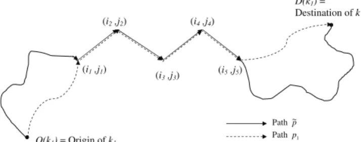
Proposition: Now suppose, without loss of

gener-ality, that path p1 ∈ Pk1 (of commodity k1) contains

arcs (i1, j1), ..., (ip, jp)∈ G, all of which have negative

time-windows with LDTj− EATi < ttij, as shown in

the Figure. Let ˜p ∈ Pk1 _{be another path of}

commod-ity k1 that has tighter time-windows than p1 on arcs

(i1, j1), ..., (ip, jp)∈ G, as shown in Figure 4. Path p~ Path p1 (i1 ,j1) (i2 ,j2) (i3 ,j3) (i4 ,j4) (i5 ,j5) O(k1) = Origin of k1 D(k1) = Destination of k1

Fig. 4 Multiple paths for commodity k1

Then, ˜p + p2+ ... + pm≤ m − 1 can also be added

to the Flow Master Problem in the same iteration.

Proof. We are given that the time-windows of ˜p

when propagated as described in Step (i) of the Schedul-ing Sub-Problem (CRTW-UU-SP) are tighter than the corresponding time-windows of p1 on arcs (i1, j1), ...,

(ip, jp)∈ G. Then, when time-windows on ˜p, p2, ..., pm

are propagated in the following steps of the Scheduling Sub-Problem to check for compatibility, the movement time windows and the final time windows in Step (vii) will be at least as tight as those for p1, p2, ..., pm.

Be-cause p1causes infeasibility, ˜p will also cause

infeasibil-ity and the constraint ˜p + p2+ ... + pm ≤ m − 1 can

also be added to the Flow Master Problem in the same iteration.

Paths of the type ˜p can be identified by a

examin-ing the network Gk1 and performing a network

modi-fication to combine arcs (i1, j1), ..., (ip, jp) into a single

arc, and examining the other paths of commodity k1

on this network. They may also be found by detecting ‘longer paths’, for example, by finding the shortest path (with all distances made negative) between O(k1) and

(i1, j1), and (i5, j5) and D(k1) as shown in the figure.

⊓ ⊔

Similarly, such paths may be found for k2 as well,

keeping p1, p3, ...pmthe same and identifying those paths

that will cause infeasibility with p1, p3, ...pm on Gk2,

etc. This is most useful when there are several paths per shipment which differ by a few arcs. In such a case, it is possible that the algorithm will try each and every alternate path in every iteration, causing the number of iterations to grow significantly. Then, adding multiple such cuts by examining the existing paths and

deter-mining more than one path of type ˜p that can cause

infeasibility can decrease the number of iterations of the algorithm.

3.11 Advantages and Disadvantages of the Decomposition Modeling Approach

Our decomposition methodology involves solving a multi-commodity Flow Master Problem and a series of network-based, easy-to-solve sub-problems. Because we are break-ing a large optimization problem into two smaller parts, one involving finding an optimal solution and the other simply finding a feasible solution, each iteration is fairly tractable. Moreover, the Scheduling Sub-Problems to ascertain whether or not a feasible schedule exists for the Flow Master Problem solution are very efficient. Polynomial-time network labeling algorithms are used, which not only identify if a feasible schedule exists, but also identify one or more constraints that can be added to the master problem to guide it towards schedule-feasible solutions. Also, specific types of additional con-straints, such as those restricting time-windows of a ve-hicle at a particular location, can be added without increasing algorithmic complexity.

The decomposition approach explicitly captures the fact that associated with any feasible solution to the CRTW-UU, there is not only one feasible schedule but in fact, a set of time-windows associated with move-ments. Upon termination of the algorithm, the schedul-ing sub-problem would have identified a set of feasi-ble time-windows corresponding to those movements. Therefore, for a solution obtained from any approach (traditional, decomposition, or other), the scheduling sub-problem can be used as a post-processing step, in order to generate windows of schedules and characterize the solution’s sensitivity to uncertainty.

Modeling uncertainty in the demand and travel time parameters using the decomposition approach does not incur much additional complexity relative to solving the CRTW for the nominal case. However, there are limi-tations in the modeling capabilities. One such is that correlations between uncertain parameters (such as be-tween travel times of adjacent links on a network) are not modeled. A second is that the choice of ‘protection levels’ for travel times on the network has to be made a priori, and involves repeated solution of instances of our model. It is possible to apply a sequential process to try increased protection levels in later iterations of the Scheduling Sub-Problem, however, it would involve a trial-and-error process on the part of the user. As in the case of the ECCP formulation of the Flow Mas-ter Problem that maximizes protection level within a budget, it would be useful to develop a mechanism to

automate the choice of path protection levels in the Scheduling Sub-Problem.

Mathematically, the presented approach always works in the feasible domain, because the set of paths for each commodity include an artificial path with high cost and zero travel time. Note that there is always a feasible but cost-maximizing solution (all commodities take their artificial paths). In practice, the use of an ar-tificial path indicates infeasibility in the sense that the related shipment(s) cannot be served within the speci-fied time-window, and these shipments will be delayed in service. They can either be delivered with an ex-panded time window, during the next day of service, or subcontracted to another carrier. The appropriate cost can be assigned for the delay, and incorporated into the Master Problem as the ‘penalty cost of not serving within the specified time window’.

Computationally, the number of iterations of the decomposition approach is sensitive to the starting so-lution to the Flow Master Problem in the first itera-tion. To speed it up, a seed solution such as one from a traditional modeling approach, or one that is being implemented by the carrier, may be provided. In case of a high degree of infeasibility in the optimal solu-tion (specifically, if several shipments cannot be served and take on artificial paths in the optimal solution) the decomposition approach can consume a lot of time iterating between the Flow Master Problem and the Scheduling Sub-Problem. This is because the Flow mas-ter Problem minimizes the penalties and maximizes the number of shipments served. It will therefore examine all possible combinations before assigning a shipment to an artificial path.

When the algorithm terminates, we always find a feasible solution. The solution contains feasible sched-ules for the routes; and moreover, all possible feasible solutions are found. To find feasible solutions more eas-ily, warm start procedures with solutions used by the carrier (even if partially infeasible) can be used.

However, if the algorithm is stopped before com-pletion, it is possible that in the current solution, a set of commodity routes have incompatible schedules with each other. This solution could be made feasible by assigning artificial paths to those shipments with in-compatible schedules that is, in practice, expand their time window and serve them late, or use an alternate (subcontracted) carrier. Another possible way to obtain a feasible solution is to use insertion heuristics to add these commodities into existing route in the solution, or create new route(s) for these commodities. Thus, the solution from the algorithm does not leave one with no solution at all, though it could be far from optimal. In

practice, this is particularly true in the case of a warm start solution.

This algorithm can be applicable for any cost struc-ture in which the objective function can be decomposed between the master Problem and the Scheduling Sub-Problem. Specifically, if the costs related to the choice of paths can be captured in the Master Problem alone, and the Scheduling problem can be cast purely as a feasibility problem, the decomposition algorithm can be used. This means that the decomposition algorithm can be used if the objective is based on cost structures that price routes based on length of routes, number of routes chosen, shipment type, etc.

4 Case Study: Truckload shipment routing and scheduling

4.1 Problem Description

Our proof-of-concept case study considers the planning of region-wide ground movements of a large pickup and delivery carrier. We consider truckload movements from a set of depots to a number of locations. The carrier owns a fleet of trucks whose movements (routes) over the network are pre-determined. However, schedules for these routes are not determined. Demands arise in the form of trailers that need to be moved from their ori-gins to their destinations on the network of vehicles. Time-windows within which the trailers should move are also specified. Shipments that are not served within the specified time-windows incur a non-service penalty. The data instance upon which most of our experiments are performed has 6 depots, 28 locations, 41 vehicles and 87 shipments in a daily schedule, and is described further in §4.4. This data set represents a medium-sized operation for this carrier. Our goal is to find a set of routes for the trailers, and schedules for truck and trailer moves; which minimize non-service costs, and are robust to uncertainty in travel times and demands.

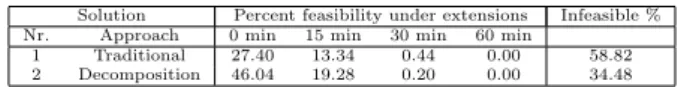
We solve this problem using the decomposition ap-proach algorithm presented in §3 and the traditional model presented in§4.2. We measure the performance of our algorithm based on various metrics: (i) number of shipments with infeasible schedules, (ii) running time of the algorithm, (ii) Percentage of scenarios requiring delivery deadline extensions of 0, 15, 30 and 60 minutes respectively to be feasible; (iii) percentage of scenarios infeasible with 60 minute extension in latest delivery time; and iv) level of robustness of solutions. To evalu-ate solution robustness, we use the simulator described in §4.3.

4.2 Traditional Approach

In this section, we present a traditional modeling ap-proach for CRTW, in which we model time as a continu-ous variable Cordeau et al. (2007). Let tibe continuous

variable representing the time at which vehicle v de-parts from node i∈ N(v)∀ v ∈ V and fk

0 represent the

artificial path for shipment k. Borrowing notation from

§2.2, the formulation of the traditional model is:

min∑ k_∈K ∑ p_∈Pk dkcpfp (33) s.t.ti+ ttkijδ p ijfp− M(1 − fp)≤ tj∀ (i, j) ∈ A, ∀ p ∈ Pk,∀ k = 0, 1, ...|K| (34) tO(k)≥ EATO(k)k (1− f

k 0) ∀ k = 0, 1, ..., |K| (35) tD(k)≤ LDTD(k)k + M (f k 0)∀ k = 0, 1, ..., |K| (36) ∑ p∈Pk fp= 1 ∀ k = 0, 1, ..., |K| (37) ∑ k∈K ∑ p∈Pk dkδijpfp≤ uij ∀ (i, j) ∈ A (38) fp∈ {0, 1} ∀ p ∈ Pk,∀ k = 0, 1, ..., |K| (39) ti≥ 0 ∀ i ∈ N. (40)

Constraints (37) - (39) form the path-based multi-commodity flow formulation that assigns a path to each shipment. Schedule related constraints (34) constrain the differences in the departure time on adjacent nodes of a vehicle or shipment path to the travel time on the arc. (35) and (36) constrain pickup and delivery of a shipment to be within the time-windows of pickup and delivery of the shipment at its origin and destination respectively.

4.3 Simulator

The simulator examines if a given solution is feasible under a set of scenarios, where each scenario comprises of a set of realized demands for shipments and a set of travel times on arcs. The simulator (41) - (49) is run once for each scenario and ttij∀ (i, j) ∈ A and dk∀ k ∈ K represent the realizations in that scenario. Let psol_k

be the path for shipment (trailer) k, for all shipments (trailers) k output by the optimization (decomposition or other) approach. Let ti be the time of departure of

the vehicle (whose path i belongs to) at each node i∈

N . Let l∈ L represent the allowable levels of extension

to the shipment delivery time, to measure degree of schedule infeasibility; and elbe the extension in minutes

allowed for level l. In our experiments we set L = 3, and