HAL Id: hal-01288772
https://hal.sorbonne-universite.fr/hal-01288772
Submitted on 15 Mar 2016
HAL is a multi-disciplinary open access archive for the deposit and dissemination of sci-entific research documents, whether they are pub-lished or not. The documents may come from teaching and research institutions in France or abroad, or from public or private research centers.
L’archive ouverte pluridisciplinaire HAL, est destinée au dépôt et à la diffusion de documents scientifiques de niveau recherche, publiés ou non, émanant des établissements d’enseignement et de recherche français ou étrangers, des laboratoires publics ou privés.
Mismatch between perceived and objectively measured
environmental obesogenic features in European
neighbourhoods
C. Roda, Hélène Charreire, Thierry Feuillet, J. d. Mackenbach, S.
Compernolle, K. Glonti, M. Ben Rebah, H. Bárdos, H. Rutter, M. Mckee, et
al.
To cite this version:
C. Roda, Hélène Charreire, Thierry Feuillet, J. d. Mackenbach, S. Compernolle, et al.. Mismatch between perceived and objectively measured environmental obesogenic features in European neigh-bourhoods. Obesity Reviews, Wiley, 2016, 17 (Supplement S1), pp.31-41. �10.1111/obr.12376�. �hal-01288772�
Mismatch Between Perceived And Objectively Measured Environmental Obesogenic Features In European Neighbourhoods
Célina Roda1, Hélène Charreire1, 2, Thierry Feuillet1, Joreintje D. Mackenbach3, Sofie Compernolle4, Ketevan Glonti5, Maher Ben Rebah1, Helga Bárdos6, Harry Rutter5, Martin McKee5, Ilse De Bourdeaudhuij4, Johannes Brug3, Jeroen Lakerveld3, Jean-Michel Oppert1, 7
1
Equipe de Recherche en Epidémiologie Nutritionnelle (EREN), Centre de Recherche en Epidémiologie et Statistiques, Inserm (U1153), Inra (U1125), Cnam, COMUE Sorbonne Paris Cité, Université Paris 13, Bobigny, France
2
Paris Est University, Lab-Urba, UPEC, Urban School of Paris, Créteil, France
3
Department of Epidemiology and Biostatistics, EMGO Institute for Health and Care Research, VU University Medical Center, Amsterdam, the Netherlands
4
Department of Movement and Sport Sciences, Faculty of Medicine and Health Sciences, Ghent University, Ghent, Belgium
5
ECOHOST – The Centre for Health and Social Change, London School of Hygiene and Tropical Medicine, London, United Kingdom
6
Department of Preventive Medicine, Faculty of Public Health, University of Debrecen, Debrecen, Hungary
7
Sorbonne Universités, Université Pierre et Marie Curie, Université Paris 06; Institute of Cardiometabolism and Nutrition, Department of Nutrition, Pitié-Salpêtrière Hospital, Assistance Publique-Hôpitaux de Paris, Paris, France
KEYWORDS: Built environment, Perception, SPOTLIGHT, Virtual audit
RUNNING TITLE: Perceived and objectively measured obesogenic environment
ACKNOWLEDGEMENTS: The authors wish to thank all survey respondents enrolled in the SPOTLIGHT project.
This work was supported by the Seventh Framework Programme (CORDIS FP7) of the European Commission, HEALTH (FP7-HEALTH-2011-two-stage) [278186]. The content of this article reflects only the authors' views and the European Commission is not liable for any use that may be made of the information contained therein.
CORRESPONDING AUTHOR: Prof. Jean-Michel Oppert Professor Jean-Michel Oppert
Department of Nutrition, Pitié-Salpêtrière Hospital (AP-HP) 47-83 Boulevard de l’Hôpital, 75013 Paris, France.
E-mail adresss: jean-michel.oppert@aphp.fr
POTENTIAL CONFLICTS OF INTEREST: None
ABBREVIATIONS: (listed in the order in which they appear) 95% CI: confidence interval at 95%
GIS: geographic information system GSV: Google Street View
MCA: multiple correspondence analysis SES: socioeconomic status
ABSTRACT
Findings from research on the association between the built environment and obesity remain equivocal, but may be partly explained by differences in approaches used to characterize the built environment. Findings obtained using subjective measures may differ substantially from those measured objectively. We investigated the agreement between perceived and objectively measured obesogenic environmental features to assess (1) the extent of agreement between individual perceptions and observable characteristics of the environment and (2) the agreement between aggregated perceptions and observable characteristics, and whether this varied by type of characteristic, region, or neighbourhood. Cross-sectional data from the SPOTLIGHT project (n=6,037 participants from 60 neighbourhoods in five European urban regions) were used. Residents’ perceptions were self-reported, and objectively measured environmental features were obtained by a virtual audit using Google Street View. Percent agreement and Kappa statistics were calculated. The mismatch was quantified at neighbourhood level by a distance metric derived from a factor map. The extent to which the mismatch metric varied by region and neighbourhood was examined using linear regression models. Overall, agreement was moderate (agreement<82%, kappa<0.3) and varied by obesogenic environmental feature, region and neighbourhood. Highest agreement was found for food outlets and outdoor recreational facilities, and lowest agreement was obtained for aesthetics. In general, a better match was observed in high residential density neighbourhoods characterized by a high density of food outlets and recreational facilities. Future studies should combine perceived and objectively measured built environment qualities to better understand the potential impact of the built environment on health, particularly in low residential density neighbourhoods.
INTRODUCTION
Findings from research on the association between characteristics of the built environment and obesity remain equivocal1–3. There are several possible explanations for these mixed results, including insufficient (or inconsistent) adjustment for lifestyle factors such as diet and sedentary behaviours, limited variability in the built environment, and heterogeneity in approaches for assessing the built environment across studies. The different approaches used to assess built environment characteristics can be grouped into two main categories: perceived, where residents’ perceptions are typically elicited from interviews or self-administered questionnaires, and objective measures derived from systematic observations (audits) or calculated from existing spatial data (e.g. street network, land-use data) using geographic information systems (GIS)4–6. A small but growing number of studies suggest that perceived and objective environments may differ substantially and can certainly not be seen as equivalent6–9.
Several studies have reported poor or moderate agreement between perceived and objectively measured obesity-related environmental characteristics8–20. Discordance tends to be greater with respondents who are older, overweight, with low income and education, less physically active, and have lived in the area for less time13,21. Certain psychosocial factors and characteristics of the social environment may also increase discordance9,22. Beyond these individual factors, physical or ‘built’ contextual factors may also play a role, i.e. the concordance between perceived and objective built-environment features may depend on which features are assessed as well as the nature of the broader physical environment. For example, a recent study reported that the association between perceived and objective built characteristics was moderated by urbanicity, i.e. in higher density areas the discordance was lower than in rural areas7. However, since existing studies were mainly conducted in Australia10,13,14,17,19,21 and North America7–9,11,15,16,20,23, the generalizability of these findings to other parts of the world is unclear.
The advent of newly-developed tools to assess the built environment offers scope to revisit this issue. Recent studies have demonstrated how remote sensing tools such as Google Street View (GSV) are feasible, affordable, and valid means to assess obesogenic environmental characteristics at street level, on a large scale at low cost24–30. Yet while GSV has been validated against other objective measures, its correlation with subjective measures is unknown. The development and validation of a virtual audit tool using GSV within Google Earth, within the framework of the EU-funded SPOTLIGHT project (www.spotlightproject.eu), provided an opportunity to assess the obesogenicity of European neighbourhoods24 and quantify its concordance with residents’ perceptions.
This study aimed to investigate the agreement between perceived (self-reported) and objectively measured (using virtual audit) obesogenic environmental features by (1) measuring agreement about
environmental features at individual level, and (2) quantifying any mismatch at neighbourhood level and how this varied by European urban region and neighbourhood.
METHODS
Study design and sampling
This study was part of the SPOTLIGHT project31 and was conducted in five urban regions across Europe: Ghent and suburbs (Belgium), Paris and inner suburbs (France), Budapest and suburbs (Hungary), the Randstad (a conurbation including the cities of Amsterdam, Rotterdam, the Hague and Utrecht in the Netherlands) and greater London (United Kingdom). Sampling of neighbourhoods and recruitment of participants have been described in detail elsewhere32. Briefly, neighbourhood sampling was based on a combination of residential density and socioeconomic status (SES) data at the neighbourhood level. This resulted in four types of pre-specified neighbourhoods: low SES/low residential density, low SES/high residential density, high SES/low residential density and high SES/high residential density. In each country, three neighbourhoods of each neighbourhood type were randomly sampled (i.e. 12 neighbourhoods per country, 60 neighbourhoods in total). Subsequently, adult inhabitants were invited to participate in a survey. The survey contained questions on demographics, neighbourhood perceptions, social environmental factors, health, motivations and barriers for healthy behaviour, obesity-related behaviours and weight and height. A total of 6,037 (10.8%, out of 55,893) individuals participated in the study between February and September 2014. The study was approved by the corresponding local ethics committees of participating countries and all participants in the survey provided informed consent.
Measures
Perceived environmental features
Perceived built environmental characteristics related to physical activity were assessed using items based on the validated ALPHA questionnaire33, supplemented with items on the food environment based on the Multi-Ethnic Study of Atherosclerosis (MESA) survey instrument34. Items on specific destinations (e.g. food outlets, recreational areas) were also included in the questionnaire. This study focused on survey items using close phrasing of virtual audit items (Table 1). The response options of items related to destinations were categorized into two categories (‘present’ or ‘not present’). Other environmental survey items that were measured on a five level ordinal scale (from ‘strongly disagree’ to ‘strongly agree’) were recoded into two categories (‘agree’ vs. ‘neither agree nor disagree and disagree’).
Objectively measured environmental features
Neighbourhood characteristics were assessed in all streets of 59 neighbourhoods (one Hungarian neighbourhood was not covered by GSV at the time of the virtual audit) and aggregated to the neighbourhood level35. Ten environmental characteristics with close phrasing of survey items were considered (Table 1). The items were related to food outlets (e.g. supermarket, restaurant), walking and cycling infrastructures (sidewalks, bicycle lanes), recreational facilities (indoor, outdoor facilities), aesthetics (graffiti/litter) and housing diversity (detached houses). Audit measures were dichotomized into two categories (‘yes’ if at least one street segment of the neighbourhood included the item considered and ‘no’ if no street segment had it).
Patterns of neighbourhood
Based on data from the virtual audit, four neighbourhood patterns had previously been identified using multiple factor and hierarchical clustering analyses35. These differ from the pre-specified types based on high/low SES and residential density used for sampling. The first cluster grouped mainly low residential density neighbourhoods (n=33) characterized by green areas (labelled ‘green neighbourhoods with low residential density’). The second cluster (n=16) also included neighbourhoods with low residential density but was characterized by features promoting active mobility (labelled ‘neighbourhoods supportive of active mobility’). The third cluster (n=7) grouped high residential density neighbourhoods with supportive food, recreational facilities, public bicycle and public transport facilities (labelled ‘high residential density neighbourhoods with food and recreational facilities’). The neighbourhoods in the fourth cluster (n=3) also had high residential density, but with graffiti and many abandoned buildings (labelled ‘high residential density neighbourhoods with low level of aesthetics’).
Self-, predefined neighbourhoods, and percent overlap
Since there is a potential discrepancy between self-defined and predefined neighbourhoods, the extent of overlap was determined. The respondents were asked to draw the boundary of their self-defined neighbourhood using an online self-mapping tool developed for this purpose (or a printout when using a paper version of the questionnaire)36. Using ArcGiS, version 10.1, software (Environmental System Research Institute, ESRI, Redlands, California)37, all neighbourhood geographical coordinate points were recorded and combined to form an enclosed area (polygon boundaries) representing the self-defined neighbourhood. GIS was also used to geolocalize home addresses and to define the administrative residential neighbourhood of each participant (defined according to small scale local administrative boundaries except for Hungary (see Lakerveld et al.32 for
more details). The percent overlap was defined as the percentage of self-defined area that fell within predefined boundaries.
Aggregated perceived environmental features at neighbourhood level
Self-reported perceptions were aggregated at neighbourhood level using a multilevel approach which allows account to be taken of individual characteristics38–40. The aggregated presence of each environmental feature in each neighbourhood (denoted ) was estimated by multilevel logistic models with two levels: one level for individuals and the other for neighbourhoods. Based on initial analysis of factors associated with perceptions9,10,16, each model was adjusted for gender, age, education level (defined as a dichotomous variable ‘high’ and ‘low’ to allow comparison across different national education systems), length of residency (dichotomized into <10 years and >=10 years) and percent overlap between pre- and self-defined neighbourhood. The model estimating aggregated perception was:
∑
where , the perception of participant i residing in neighbourhood j; , the mean of
neighbourhood perception (across all study neighbourhoods); q, the number of individual-level adjusters; X, the adjusters; , the regression coefficients associated with the adjusters; , the
neighbourhood variance; and , the individual variance. The neighbourhood-level residuals
indicate the degree to which perception of neighbourhood j differs from the mean . According to
de Jong et al. (2011)39, the perceived presence of a given environmental feature in each neighbourhood was calculated by:
Statistical analysis
Agreement between survey and virtual audit items at individual level
Agreement between survey and virtual audit items was assessed by percent agreement and Cohen’s Kappa statistics. The percent of agreement was calculated to represent a basic measure of the proportion of respondents that accurately perceived the presence or absence of an environmental feature in their neighbourhood. Kappa statistics were then calculated to measure the proportion of observed agreement that occurs beyond chance41. According to Landis and Koch42, the strength of agreement for each item-pair was classified as: poor (kappa less than 0), slight (0.00-0.20), fair (0.21-0.40), moderate (0.41 and 0.60), substantial (0.61 and 0.80), and almost perfect (0.81 and 1.00).
Determination of the mismatch metric at neighbourhood level
The mismatch between aggregated perceptions and objectively measured data on many neighbourhood environmental features was quantified through a factor analysis. Multiple correspondence analysis (MCA) can be considered to be a generalization of principal component analysis for categorical variables43. MCA was performed on 2x59 observations (2 observations per neighbourhood: perceived and objectively measured) with 10 environmental features. The observations were then plotted in a bi-dimensional space (factor map) to measure the distances between perceived and objectively measured data for each neighbourhood. These distances reflect the similarities between the observations. A total of 59 distances (1 distance per neighbourhood) was determined. The metric, derived from these distances, quantified the match/mismatch at neighbourhood level.
Relation between mismatch metric and environmental factors (regions, neighbourhood types and patterns)
Normality of the distribution of the mismatch metric was assessed using the Shapiro–Wilk test and Henry’s graphical method. As the distribution was log-normal, results are shown as geometric means with their geometric standard deviation. Median with 25th and 75th percentiles are also shown to summarize the metric. Comparisons were based on parametric tests. The differences in mismatch between regions, neighbourhood types and patterns were examined using Student t-test and analysis of variance (ANOVA) with post-hoc Bonferroni tests.
Additionally, relations between the mismatch metric and environmental variables were assessed by linear regressions (Model 1 included European regions and neighbourhood types, and Model 2 included neighbourhood patterns – this variable provides a better characterization of the neighbourhoods). The explained variance of the mismatch by region, neighbourhood type and pattern was expressed as the determination coefficient (R²). Results from multivariate linear regressions were summarized by adjusted regression coefficients (β) with their confidence intervals at 95% (95% CI).
Sensitivity analysis
In order to examine the potential impact of the percent overlap between self-defined and predefined neighbourhood, the analyses were also conducted without adjustment for percent overlap in the aggregation of self-reported perceptions at neighbourhood level.
Statistical analyses were performed with R (FactoMineR package44), version 3.2 (R Development Core Team, 2010)45 and STATA statistical software (release 13.0; Stata Corporation, College Station, TX, USA).
RESULTS
Agreement between residents’ perceptions and objectively measured environmental features
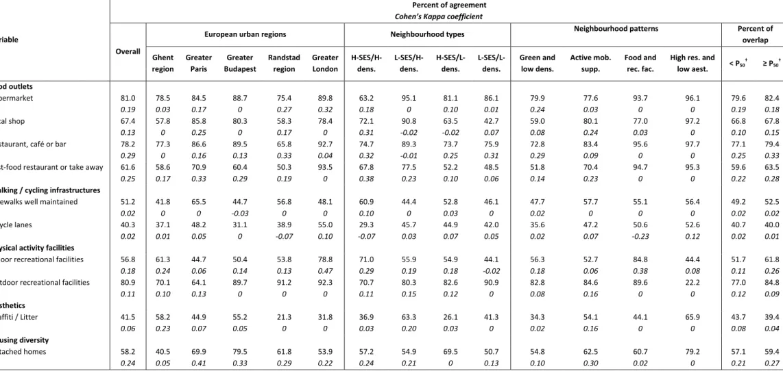
Table 2 presents agreement for the 10 item-pairs. Overall, the percent of agreement was relatively high for items related to formal facilities (food outlets: from 61.6% to 81.1%, and physical activity facilities: from 56.8% to 81.0%) compared with informal or more subjective qualities of the neighbourhood (housing diversity: 58.2%, walking/cycling infrastructures: from 40.3% to 51.2%, and aesthetics: 41.5%). However, kappa indicated poor or fair agreement (kappa<0.3).
Percent agreement differed across European regions. The highest levels of agreement for food outlets (except for local shops), physical activity facilities and bicycle lanes were observed in greater London. The highest level of agreement for well-maintained sidewalks was observed in greater Paris. For aesthetics and housing diversity, the highest percent was found in Ghent region and greater Budapest, respectively. Concerning neighbourhood types, for all food outlets, and graffiti/litter the percent of agreement was higher in low SES/high residential density neighbourhoods. With regard to physical activity facilities, highest agreement was observed in high SES/high residential density neighbourhoods for indoor recreational facilities, and in low SES/low density neighbourhoods for outdoor recreational facilities. The highest levels of agreement for well-maintained sidewalks and for detached homes were observed in high SES/high density neighbourhoods, and high SES/low density neighbourhoods, respectively. In regard to neighbourhood patterns, the highest levels of agreement were mainly observed in neighbourhoods labelled ‘food and recreational facilities’ or ‘high residential and low aesthetics’. The highest level of agreement for recreational facilities was obtained for ‘food and recreational facilities’ neighbourhoods. The agreement of food outlets, housing density and graffiti/litter was higher in ‘high residential and low aesthetics’ neighbourhoods compared to other neighbourhood patterns. Finally, except for bicycle lanes and graffiti/litter, a better agreement was observed when there was more overlap in the two definitions of neighbourhood.
Mismatch metric and environmental determinants
The geometric mean (geometric standard deviation) and median (P25-P75) of the mismatch metric were equal to 0.89 (1.72) and 0.88 (0.60-1.38) respectively (Table 3). In bivariate analyses (Table 3), the mismatch was similar in each European region. There was no difference with neighbourhood SES but the mismatch was significantly higher in low residential density neighbourhoods compared with
neighbourhoods was stronger using neighbourhood patterns (ANOVA, p-value<0.001). The distance between perceived and objectively measured data was significantly smaller in neighbourhoods labelled as ‘food and recreational facilities’ compared with neighbourhoods from the ‘green and low density’ cluster (Bonferroni test, p-value=0.001). Although slightly attenuated, these differences were also observed when percent of overlap was not taken into account in the aggregation of perceptions at neighbourhood level (Table S1). In multivariate analyses (Figure 1), the relation with residential density remained significant, and the mismatch was lower in greater London compared with the Ghent region (Model 1, R2=19.9%). The mismatch was significantly lower in neighbourhoods grouped into the clusters labelled ‘food and recreational facilities’ and ‘high residential and low aesthetics’ than in neighbourhoods from the ‘green and low density’ cluster (Model 2, R2=26.6%). The sensitivity analysis confirmed these relations (Figure S1).
DISCUSSION
This study investigated the agreement between residents’ perceptions (based on a survey among residents of the neighbourhoods) and objectively measured data (based on a virtual audit of residential neighbourhoods) of potentially obesogenic environmental features. The study went beyond the traditional focus on agreement at individual level to consider aggregate differences at neighbourhood level and how they varied across five European urban regions and in different types of neighbourhoods. Agreement varied by obesity-related features and neighbourhoods. A better match was observed in high residential density neighbourhoods characterized by a high density of food and recreational facilities compared with other types of neighbourhoods.
Our study is in line with previous studies showing low or moderate agreement between subjective and objective measures. However it is the first to assess concordance between residents’ perceptions collected by questionnaire and virtual audit data using GSV in different regions. Previously, residents’ ratings of neighbourhood features were usually compared with objective indicators obtained from observational field audits8, GIS or through publicly available information10,11,13,15,16,18–20. Lower agreement was documented when distance/access to amenities and subjective aspects were examined compared with self-reported presence/absence of a given facility. For instance, matching between perceived and objective proximity to the closest park was observed with only 18% of participants (kappa=0.01) in Ontario16. For distance to supermarkets the discordance amounted to 31.5% among low-income housing residents in greater Boston12. Concerning walkability (defined by dwelling density, street connectivity, land-use, and retail density), around a third of participants showed non-concordance between measures (i.e. perceiving more highly walkable areas as low; or
contrast, a high percent of agreement (from 50% to 91%) for non-residential destinations (e.g. parks, grocery stores, pools) was documented in Wisconsin7. Our results are consistent with these findings in that a higher percent of agreement was observed for formal facilities (i.e. destinations), and lower agreement was found for informal or more subjective qualities of the neighbourhood (i.e. items related to aesthetics). Higher agreement for destinations or facilities, such as recreational facilities and food outlets may be due to the fact that residents may be more familiar with such facilities because these are ‘used’ in everyday life, and their presence is thus more obvious. Conversely, environmental features related to aesthetics - such as the presence of litter or graffiti - are not used, but should be noted, and are possibly also more subjective. i.e. a food outlet is there or not, but the smallest amount of litter may be noted as such by some, while other will report on litter only if present in larger amounts. It is interesting to note that aesthetic items had already been found to have the lowest value of agreement in the SPOTLIGHT virtual audit tool validation24.
In contrast to previous studies in which agreement on environmental features was analysed separately, the mismatch was quantified here at the neighbourhood level by a distance metric obtained by factor analysis. With this approach the multifactorial aspects of the built environment were taken into account. Although the study was limited to environmental features of which the phrasing of questions/items in the virtual audit measures were close to the self-reported residents’ measures, the main aspects of the built environment were considered (food outlets, physical activity facilities, aesthetics, housing diversity). In addition, individual characteristics previously suggested to be associated with perceptions (e.g. gender, education level, age, length of residency) were taken into account in the multilevel models employed to aggregate residents’ perceptions at neighbourhood level. These models were also adjusted for the percent overlap. In previous studies, authors assessed objective measures within the nearest boundary and/or buffers (Euclidian and/or street network buffers) surrounding respondents’ residence, assuming that this predefined area is comparable with a participant’s perceived neighbourhood7,9–12,16. Nevertheless, Coulton et al.46,47 have documented discrepancies between researcher and resident defined neighbourhood boundaries. In our study, predefined neighbourhoods did not overlap completely with self-defined neighbourhoods: the median overlap was 21.2%. Since the mismatch between predefined and self-defined neighbourhood boundaries is potentially associated with discordance between perceived and objectively measured environmental features, the aggregated residents’ perceptions were adjusted for the percent overlap in our study. Nevertheless, the impact of the adjustment for percent overlap on results at neighbourhood level is limited because the results are mainly the same whether or not the overlap is taken into account.
Agreement was found to differ across European regions and neighbourhoods. International differences may reflect national differences in built environment characteristics48. The mismatch was significantly lower in high residential density neighbourhoods compared with low residential density neighbourhoods. Higher density generally results in more compact neighbourhoods and higher provision of local resources and destinations such as supermarkets and recreational amenities49. This relation was confirmed by the analysis of neighbourhood patterns35. Mismatch was smaller for clusters that exclusively grouped high residential density neighbourhoods, characterized by the presence of food and recreational facilities and low aesthetics. The higher mismatch observed in Ghent region compared with London region is in line with the previously described differences in environmental characteristics between these regions35.
A potential limitation of this study was that objectively measured data were not collected at participant level (i.e. using self-defined neighbourhoods) but at predefined neighbourhood level (i.e. using administrative neighbourhoods) in each country. Results found in aggregated data at neighbourhood level cannot be extrapolated to individual level because associations may or may not be the same, according to the “ecological fallacy”50. In a study of this scale it would be extremely time consuming to perform a virtual audit in each self-defined neighbourhood. In addition to the cross-sectional design, another limitation of this study was the slight difference in wording used to describe environmental features in the two measures (i.e. survey and virtual audit) limiting assessment of agreement to certain item-pairs only, but multiple dimensions of the obesogenic environment (food outlets, physical activity facilities, aesthetics, housing diversity) were covered. Despite the above mentioned limitations, this study also has a number of strengths. To our knowledge, this study quantified for the first time mismatch at neighbourhood level by comparing aggregated residents’ perceptions and objectively measured data from an innovative and comprehensive validated virtual audit tool24. Additionally, perceptions of environmental features were collected from a large population in the audited areas. The standardized data collection (survey and virtual audit and) across heterogeneous neighbourhoods led to a comparison of different measures of built environment across European regions and neighbourhoods.
In conclusion, this study shows moderate agreement between perceived (residents’ perceptions) and objectively measured (based on a virtual audit) obesogenic built environment features. Furthermore, we found evidence that concordance differed across neighbourhoods, with the highest concordance found in high residential density neighbourhoods characterized by food outlets and recreational facilities. Researchers examining the relations between the built environment and obesity-related
behaviours and health outcomes should be aware of the potential lack of concordance between assessment approaches. While objective measures provide a clear picture of the built environment, it is also important to assess people’s perceptions, especially in neighbourhoods with low residential density, because they may mediate the relations between the built environment and behaviours. Understanding a lack of concordance is critical to investigate with more accuracy the relations between the built environment and health in order to design more effective and comprehensive interventions.
REFERENCES
1 Papas MA, Alberg AJ, Ewing R et al. The built environment and obesity. Epidemiol Rev 2007; 29: 129–143.
2 Feng J, Glass TA, Curriero FC et al. The built environment and obesity: a systematic review of the epidemiologic evidence. Health Place 2010; 16: 175–190.
3 Mackenbach JD, Rutter H, Compernolle S et al. Obesogenic environments: a systematic review of the association between the physical environment and adult weight status, the SPOTLIGHT project. BMC Public Health 2014; 14: 233.
4 Brownson RC, Hoehner CM, Day K et al. Measuring the Built Environment for Physical Activity. Am J Prev Med 2009; 36: S99–123.e12.
5 Charreire H, Casey R, Salze P et al. Measuring the food environment using geographical information systems: a methodological review. Public Health Nutr 2010; 13: 1773–1785.
6 Lin L, Moudon AV. Objective versus subjective measures of the built environment, which are most effective in capturing associations with walking? Health Place 2010; 16: 339–348.
7 Bailey EJ, Malecki KC, Engelman CD et al. Predictors of discordance between perceived and objective neighborhood data. Ann Epidemiol 2014; 24: 214–221.
8 Boehmer TK, Hoehner CM, Deshpande AD et al. Perceived and observed neighborhood indicators of obesity among urban adults. Int J Obes 2005 2007; 31: 968–977.
9 Ma L, Dill J. Associations between the objective and perceived built environment and bicycling for transportation. J Transp Health 2015; 2: 248–255.
10 Ball K, Jeffery RW, Crawford DA et al. Mismatch between perceived and objective measures of physical activity environments. Prev Med 2008; 47: 294–298.
11 Barnes TL, Bell BA, Freedman DA et al. Do people really know what food retailers exist in their neighborhood? Examining GIS-based and perceived presence of retail food outlets in an eight-county region of South Carolina. Spat Spatio-Temporal Epidemiol 2015; 13: 31–40.
12 Caspi CE, Kawachi I, Subramanian SV et al. The relationship between diet and perceived and objective access to supermarkets among low-income housing residents. Soc Sci Med 1982 2012; 75: 1254–1262.
13 Gebel K, Bauman A, Owen N. Correlates of non-concordance between perceived and objective measures of walkability. Ann Behav Med Publ Soc Behav Med 2009; 37: 228–238.
14 Gebel K, Bauman AE, Sugiyama T et al. Mismatch between perceived and objectively assessed neighborhood walkability attributes: prospective relationships with walking and weight gain. Health Place 2011; 17: 519–524.
15 Kirtland KA, Porter DE, Addy CL et al. Environmental measures of physical activity supports: perception versus reality. Am J Prev Med 2003; 24: 323–331.
16 Lackey KJ, Kaczynski AT. Correspondence of perceived vs. objective proximity to parks and their relationship to park-based physical activity. Int J Behav Nutr Phys Act 2009; 6: 53.
17 Leslie E, Sugiyama T, Ierodiaconou D et al. Perceived and objectively measured greenness of neighbourhoods: Are they measuring the same thing? Landsc Urban Plan 2010; 95: 28–33.
18 Macintyre S, Macdonald L, Ellaway A. Lack of agreement between measured and self-reported distance from public green parks in Glasgow, Scotland. Int J Behav Nutr Phys Act 2008; 5: 26.
19 McCormack GR, Cerin E, Leslie E et al. Objective Versus Perceived Walking Distances to Destinations Correspondence and Predictive Validity. Environ Behav 2008; 40: 401–425.
20 McGinn AP, Evenson KR, Herring AH et al. Exploring associations between physical activity and perceived and objective measures of the built environment. J Urban Health Bull N Y Acad Med 2007; 84: 162–184.
21 Koohsari MJ, Badland H, Sugiyama T et al. Mismatch between perceived and objectively measured land use mix and street connectivity: associations with neighborhood walking. J Urban Health Bull N Y Acad Med 2015; 92: 242–252.
22 Kamphuis CBM, Mackenbach JP, Giskes K, Huisman M, Brug J, van Lenthe FJ. Why do poor people perceive poor neighbourhoods? The role of objective neighbourhood features and psychosocial factors. Health Place 2010; 16: 744–754.
23 Boehmer TK, Hoehner CM, Wyrwich KW et al. Correspondence between perceived and observed measures of neighborhood environmental supports for physical activity. J Phys Act Health 2006; 3: 22.
24 Bethlehem JR, Mackenbach JD, Ben-Rebah M et al. The SPOTLIGHT virtual audit tool: a valid and reliable tool to assess obesogenic characteristics of the built environment. Int J Health Geogr 2014; 13: 52.
25 Charreire H, Mackenbach JD, Ouasti M et al. Using remote sensing to define environmental characteristics related to physical activity and dietary behaviours: a systematic review (the SPOTLIGHT project). Health Place 2014; 25: 1–9.
26 Curtis JW, Curtis A, Mapes J et al. Using Google Street View for systematic observation of the built environment: analysis of spatio-temporal instability of imagery dates. Int J Health Geogr 2013; 12: 53.
27 Griew P, Hillsdon M, Foster C et al. Developing and testing a street audit tool using Google Street View to measure environmental supportiveness for physical activity. Int J Behav Nutr Phys Act 2013; 10: 103.
28 Kelly CM, Wilson JS, Baker EA et al. Using Google Street View to audit the built environment: inter-rater reliability results. Ann Behav Med Publ Soc Behav Med 2013; 45 Suppl 1: S108–112. 29 Odgers CL, Caspi A, Bates CJ et al. Systematic social observation of children’s neighborhoods
using Google Street View: a reliable and cost-effective method. J Child Psychol Psychiatry 2012; 53: 1009–1017.
30 Rundle AG, Bader MDM, Richards CA et al. Using Google Street View to audit neighborhood environments. Am J Prev Med 2011; 40: 94–100.
31 Lakerveld J, Brug J, Bot S et al. Sustainable prevention of obesity through integrated strategies: The SPOTLIGHT project’s conceptual framework and design. BMC Public Health 2012; 12: 793.
32 Lakerveld J, Ben-Rebah M, Mackenbach JD et al. Obesity-related behaviours and BMI in five urban regions across Europe: sampling design and results from the SPOTLIGHT cross-sectional survey. BMJ Open. 2015; 5:e008505.doi:10.1136/bmjopen-2015-008505.
33 Spittaels H, Foster C, Oppert J-M et al. Assessment of environmental correlates of physical activity: development of a European questionnaire. Int J Behav Nutr Phys Act 2009; 6: 39.
34 Curl CL, Beresford SAA, Hajat A et al. Associations of organic produce consumption with socioeconomic status and the local food environment: Multi-Ethnic Study of Atherosclerosis (MESA). PloS One 2013; 8: e69778.
35 Feuillet T, Charreire H, Roda C, Ben-Rebah M, Mackenbach JD, Compernolle S et al. Neighbourhood patterns based on virtual audit of environmental obesogenic characteristics (the SPOTLIGHT project). Obes Rev 2016; 17(Suppl. 1): 19–30.
36 Charreire H, Feuillet T, Roda C et al. Self-defined residential neighbourhoods: size variations and correlates across 5 European urban regions (The Spotlight project). Obes Rev 2016; 17(Suppl. 1): 9–18.
37 Environmental Systems Research Institute. ArcGIS 10.1. Redlands, CA, 2012.
38 Mohnen SM, Groenewegen PP, Völker B et al. Neighborhood social capital and individual health. Soc Sci Med 1982 2011; 72: 660–667.
39 de Jong K, Albin M, Skärbäck E et al. Area-aggregated assessments of perceived environmental attributes may overcome single-source bias in studies of green environments and health: results from a cross-sectional survey in southern Sweden. Environ Health Glob Access Sci Source 2011; 10: 4.
40 Mujahid MS, Diez Roux AV, Morenoff JD et al. Assessing the measurement properties of neighborhood scales: from psychometrics to ecometrics. Am J Epidemiol 2007; 165: 858–867. 41 Fleiss JL. Statistical Methods for Rates and Proportions. Wiley, 1981.
42 Landis JR, Koch GG. The measurement of observer agreement for categorical data. Biometrics 1977; 33: 159–174.
43 Husson F, Le S, Pages J. Exploratory Multivariate Analysis by Example Using R. CRC Press: Boca Raton, 2010.
44 Lê S, Rennes A, Josse J et al. FactoMineR: an R package for multivariate analysis. J Stat Softw 2008; : 1–18.
45 R Core Team. R: A language and environment for statistical computing. R Foundation for Statistical Computing, Vienna, Austria, 2015.
46 Coulton CJ, Korbin J, Chan T et al. Mapping residents’ perceptions of neighborhood boundaries: a methodological note. Am J Community Psychol 2001; 29: 371–383.
47 Coulton CJ, Jennings MZ, Chan T. How big is my neighborhood? Individual and contextual effects on perceptions of neighborhood scale. Am J Community Psychol 2013; 51: 140–150. 48 Adams MA, Frank LD, Schipperijn J et al. International variation in neighborhood walkability,
transit, and recreation environments using geographic information systems: the IPEN adult study. Int J Health Geogr 2014; 13: 43.
49 Giles-Corti B, Hooper P, Foster S et al. Evidence Review: Low density development: Impacts on physical activity and associated health outcomes. National Heart Foundation of Australia, 2014; 1–53.
50 Szklo M, Nieto J. Epidemiology: Beyond the Basics. Jones & Bartlett Publishers, Burlington 2012.
TABLES AND FIGURE
Table 1. Correspondence between perceived (survey) and objectively measured (virtual audit) environmental features and prevalence of the items
Table 2. Agreement* between perceived (survey) and objectively measured (virtual audit) environmental features according to European regions, neighbourhoods (types and patterns) and percent of overlap
Table 3. Mismatch metric levels and differences across European regions, neighbourhood types (based on socioeconomic level and residential density) and neighbourhood patterns
Figure 1. Associations between mismatch metric (log-transformed) and European urban regions, neighbourhood types (based on socioeconomic level and residential density - Model 1), and neighbourhood patterns (Model 2). Results from multivariate linear regression models
Determination coefficient of the linear regression models (R²) were 19.9% (model 1), and 26.6% (model 2) Intercepts (95% CI) were equal to 0.11 (-0.25 ; 0.46) in model 1, and equal to 0.09 (-0.08 ; 0.25) in model 2 β: estimated regression coefficient
95% CI: confidence interval at 95%
SUPPORTING INFORMATION
Table S1. Mismatch metric levels and differences across European regions, neighbourhood types (based on socioeconomic level and residential density) and neighbourhood patterns (perceptions not adjusted for the percent overlap between self- and predefined neighbourhood)
Figure S1. Associations between mismatch metric (log-transformed) and European urban regions, neighbourhood types (based on socioeconomic level and residential density - Model 1), and neighbourhood patterns (Model 2). Results from multivariate linear regression models (perceptions not adjusted for the percent overlap between self- and predefined neighbourhood)
Determination coefficient of the linear regression models (R²) were 20.4% (model 1), and 24.2% (model 2) Intercepts (95% CI) were equal to 0.05 (-0.31 ; 0.41) in model 1, and 0.06 (-0.11 ; 0.23) in model 2 β: estimated regression coefficient
Table 1. Correspondence between perceived (survey) and objectively measured (virtual audit) environmental features and prevalence of the items
Variable Survey Virtual audit
Question phrasing N=3914
†
n (%) Question phrasing
N=59 n (%)
Are any of the following local business or facilities present in your neighbourhood? % segments with the item in the neighbourhood
Food outlets Supermarket
Local shop (grocery shop, bakery, butcher, fruit/vegetable shop etc.) Restaurant, café or bar
Fast-food restaurant or take away
3308 (86.6) 3413 (89.5) 3144 (85.3) 2565 (71.5)
Supermarket
Local shop (bakery, fish-shop, butcher, greengrocer) Restaurant, café/bar*
Fast-food restaurant, take away*
51 (86.4) 41 (69.5) 46 (78.0) 31 (52.5) Walking, cycling infrastructures
Agreement with statement on characteristics of neighbourhood % segments with the item in the neighbourhood
“The pavements in my neighbourhood are well maintained”
“There are special lanes, routes or paths for cycling in my neighbourhood”
1852 (50.2) 2592 (68.2)
Sidewalk (presence and ‘good’ maintenance) Bicycle lane
56 (94.2) 13 (22.0)
Physical activity facilities
Are any of the following local business or facilities present in your neighbourhood? % segments with the item in the neighbourhood
Leisure facility such as gym, swimming pool Open recreation area (such as a park or playing field)
2388 (65.4) 3251 (87.7)
Indoor recreational facilities (e.g. gym, swimming pool, sports hall) Outdoor recreational facilities, public park*
22 (37.3) 52 (88.1)
Aesthetics Agreement with statement on characteristics of neighbourhood % segments with the item in the neighbourhood
“My neighbourhood is generally free from litter, rubbish or graffiti” 1285 (33.8) Graffiti, litter* 52 (88.1)
Housing diversity
Agreement with statement on characteristics of neighbourhood % segments with the item in the neighbourhood
“There are many detached houses in my neighbourhood” 1540 (40.5) Detached / semidetached homes 45 (76.3)
*initial items were aggregated to make wording similar to data collected in the survey
†
participants who provided data on self-defined neighbourhoods boundaries and for whom the overlap between administrative limits and self-defined neighbourhoods was determined N per variable may vary because of missing values
Table 2. Agreement* between perceived (survey) and objectively measured (virtual audit) environmental features according to European regions, neighbourhoods (types and patterns) and percent of overlap
Variable
Percent of agreement
Cohen’s Kappa coefficient
Overall
European urban regions Neighbourhood types Neighbourhood patterns Percent of
overlap Ghent region Greater Paris Greater Budapest Randstad region Greater London H-SES/H-dens. L-SES/H-dens. H-SES/L-dens. L-SES/L-dens. Green and low dens. Active mob. supp. Food and rec. fac.
High res. and low aest. < P50 † ≥ P50† Food outlets Supermarket 81.0 0.19 78.5 0.03 84.5 0.17 88.7 0 75.4 0.27 89.8 0.32 63.2 0.18 95.1 0 81.1 0.10 86.1 0.01 79.9 0.24 77.6 0.03 93.7 0 96.1 0 79.6 0.19 82.4 0.18 Local shop 67.4 0.13 57.8 0 85.8 0.25 80.3 0 58.3 0.17 78.4 0 72.1 0.31 90.8 -0.02 63.5 -0.02 42.7 0.07 59.0 0.08 80.1 0.24 77.0 0.03 97.2 0 66.8 0.10 67.8 0.15
Restaurant, café or bar 78.2
0.29 77.3 0 86.6 0.16 89.5 0.13 65.8 0.33 92.7 0.04 74.7 0.32 89.3 -0.01 73.7 0.25 75.9 0.31 72.8 0.29 83.4 0.09 95.6 0 97.7 0 77.1 0.25 79.4 0.33
Fast-food restaurant or take away 61.6
0.25 58.6 0.17 70.9 0.33 60.4 0.29 50.3 0.19 93.5 0 67.8 0.38 77.5 0.23 52.2 0.10 48.5 0.06 51.8 0.14 70.4 0.23 94.7 0 95.3 0 59.6 0.22 63.5 0.28
Walking / cycling infrastructures
Sidewalks well maintained 51.2
0.02 41.8 0 65.5 0 44.7 -0.03 56.8 0 48.1 0 60.9 0.10 44.4 0 52.8 0.03 46.1 0 47.7 0.02 57.7 0 55.1 0 56.4 0 49.2 0.02 52.5 0.02 Bicycle lanes 40.3 0.02 37.1 0.01 48.2 0.05 31.1 0 38.9 -0.07 55.0 0.10 29.3 -0.07 45.7 0.03 44.9 0.07 42.0 0.05 35.6 0.02 47.2 0.07 50.6 -0.23 52.6 0.12 40.7 0.02 40.0 0.01
Physical activity facilities
Indoor recreational facilities 56.8
0.18 61.3 0.24 44.7 0.06 50.4 0.14 53.8 0.13 78.8 0.47 71.0 0.29 55.9 0.19 54.9 0.18 44.1 -0.02 56.3 0.18 52.7 0.06 84.8 0.38 44.4 0.08 51.7 0.11 61.8 0.26
Outdoor recreational facilities 80.9
0.11 70.1 0.10 64.1 0.13 89.7 0 91.2 0 92.3 0 70.7 0.11 80.3 0.15 82.6 0.12 90.9 0 82.8 0.08 84.6 0.16 89.6 0 22.2 0 77.0 0.12 84.8 0.09 Aesthetics Graffiti / Litter 41.5 0.06 58.2 0.23 44.9 0.07 55.2 0.05 21.3 0 31.8 0 36.9 0.03 63.3 0.20 26.1 0.03 41.3 0 34.3 0.02 54.1 0.16 44.1 0 65.9 0 43.7 0.08 39.4 0.04 Housing diversity Detached homes 58.2 0.24 40.5 0.05 69.9 0.41 79.5 0.33 61.8 0.29 53.9 0.22 57.2 0.24 54.9 0.21 69.5 0 50.7 0.13 54.8 0.10 62.5 0.30 60.7 0.02 79.2 0 57.1 0.21 59.4 0.27
*assessed by the percent of agreement and the Cohen’s Kappa coefficient. The values in the first line are the percent of agreement between perceived (survey) and objectively measured (GSV) items of environmental features. The values in the second line (in italic) are the Cohen’s Kappa coefficients.
†
Table 3. Mismatch metric levels and differences across European regions, neighbourhood types (based on socioeconomic level and residential density) and neighbourhood patterns.
n GM (GSD) Median (P25-P75) p-value
All neighbourhoods 59 0.89 (1.72) 0.88 (0.60-1.38) -
European urban regions
Ghent region 12 1.00 (1.79) 0.96 (0.82-1.61) 0.215 Greater Paris 12 0.91 (1.59) 0.88 (0.73-1.32) Greater Budapest 11 0.90 (1.54) 0.88 (0.58-1.38) Ransdstad region 12 1.06 (1.78) 1.12 (0.81-1.63) Greater London 12 0.65 (1.80) 0.63 (0.52-0.93)
Neighbourhood residential density
Low 29 1.05 (1.54) 1.08 (0.86-1.51)
0.023
High 30 0.76 (1.82) 0.80 (0.56-1.03)
Neighbourhood socioeconomic level
Low 29 0.84 (1.75) 0.86 (0.58-1.16)
0.402
High 30 0.95 (1.69) 0.88 (0.68-1.51)
Neighbourhood patterns
Green and low density 33 1.09 (1.57) 1.08 (0.86-1.66)†
<0.001
Active mobility supportive 16 0.84 (1.69) 0.86 (0.70-1.25)
Food and recreational facilities 7 0.49 (1.63) 0.57 (0.30-0.58)†
High residential and low aesthetics 3 0.57 (1.66) 0.66 (0.33-0.87)
GM: geometric mean
GSD: geometric standard deviation Px: xth percentile
p-value of Student’s-test or ANOVA on log-transformed mismatch metric
†