HAL Id: halshs-01130403
https://halshs.archives-ouvertes.fr/halshs-01130403
Submitted on 11 Mar 2015
HAL is a multi-disciplinary open access archive for the deposit and dissemination of sci-entific research documents, whether they are pub-lished or not. The documents may come from teaching and research institutions in France or abroad, or from public or private research centers.
L’archive ouverte pluridisciplinaire HAL, est destinée au dépôt et à la diffusion de documents scientifiques de niveau recherche, publiés ou non, émanant des établissements d’enseignement et de recherche français ou étrangers, des laboratoires publics ou privés.
Paul Cahu, Falilou Fall, Roland Pongou
To cite this version:
Paul Cahu, Falilou Fall, Roland Pongou. Beauty, Polygyny and Fertility: Theory and Evidence. 2014. �halshs-01130403�
Documents de Travail du
Centre d’Economie de la Sorbonne
Beauty, Polygyny, and Fertility: Theory and Evidence
Paul CAHU, Falilou FALL, Roland PONGOU
2014.78
Beauty, Polygyny, and Fertility: Theory and Evidence
Paul Cahu, Falilou Fall, and Roland Pongou1
This Version: September 2014
Abstract: We propose a simple model of a mating economy in both monogamous and
polygynous cultures, and derive implications for how polygyny a¤ects individual and aggregate fertility. We …nd that an attractive woman is more likely to …nd a high-status husband. However, when polygyny is allowed, high-status husbands naturally attract other women; this implies that female beauty increases the likelihood of entering into a polygynous relationship. A woman in a polygynous relationship produces fewer children than a woman in a monogamous relationship as long as the preference for reproduction relative to consumption is not too strong. However, the societal practice of polygyny increases aggregate fertility through two distinct channels: (1) by increasing the number of marriages; and (2) by triggering fertility contagion: a woman, whether involved in a monogamous or polygynous relationship, produces more children as polygyny becomes more prevalent in her neighborhood. We empirically validate each of the model’s key predictions.
Keywords: Mating Economy, Monogamy, Polygyny, Beauty, Status, Fertility, Contagion, Networks
JEL Classi…cation: A13, C78, J12, J13, Z10
1Paul Cahu (p.cahu@eib.org) is at the European Investment Bank; Falilou Fall (falilou.fall@univ-paris1.fr)
is at Centre d’Economie de la Sorbonne, Université Paris 1; and Roland Pongou (roland.pongou@uottawa.ca) is at the Department of Economics of the University of Ottawa. Fairooz Reaz provided excellent research assistance. We thank Ingela Alger, Jakina Debnam, Marcel Fafchamps, James Fenske, Andrew Foster, Isaac Mbiti, Pierre Evariste Nguimkeu, Pauline Rossi, Paul Schultz, Michel Tenikue, Leonard Wantchekon, Joshua Wilde, and several participants at the Conference on the Economics of the Family in Paris and the CSAE conference at the University of Oxford for useful comments and suggestions. Falilou Fall acknowledges …nancial support from the H. d’Albis European Research Council (ERC Stg Grant DU 283953). Roland Pongou acknowledges research grant from the Social Sciences and Humanities Research Council of Canada.
1
Introduction
The maternal instinct leads a woman to prefer a tenth share in a …rst rate man to the exclusive possession of a third rate –George Bernard Shaw In Maxims for Revolutionists (1903)
The last …ve decades have witnessed an important growth of the literature on two-sided matching and its applications to the marriage market. Most studies, however, have focused on the formation of relationships in monogamous societies, with little attention paid to polygyny, a form of plural marriage involving one man and more than one woman, which has existed for millennia and continues to exist in many contemporary societies. Therefore, di¤erences in marriage patterns and outcomes across societies with di¤erent matrimonial cultures have not been su¢ ciently studied. In this paper, we propose a simple model of a mating economy to analyze and compare marriage in monogamous and polygynous societies. We subsequently derive implications for how polygyny a¤ects male and female fertility at both the individual and aggregate levels.
The focus on fertility as an outcome naturally comes from the fact that the desire for progeny is generally regarded as one of the strongest appeals of polygyny: a large number of children in a household constitutes an important workforce, ensures family continuity through reproduction, and brings prestige to parents. However, the question of how polygyny a¤ects fertility has not been resolved in the literature. Tertilt (2005) …nds that women living in polygynous countries have 2.2 more children than those in monogamous countries. In an earlier work, however, Muhsam (1956) found that the number of children was 32 percent lower for women married to polygynous men than for their counterparts married to monogamous men. Busia (1954), on the other hand, found no signi…cant di¤erence in the fertility of women in monogamous relationships and those married to polygynists.
These previous studies clearly show that the e¤ect of polygyny on fertility varies signi…-cantly, and may also depend on whether it is assessed at the individual level or at the aggregate level. There is therefore a need to understand the mechanism through which polygyny a¤ects fertility. Ideally, such a mechanism should also shed light on the characteristics of individ-uals who choose to be involved in a polygynous marriage, and elucidate the role that these individual characteristics play in the relationship between polygyny and fertility.
1.1
An overview of the model
The model proposed in this paper assumes a world in which agents marry in the …rst period and produce children in the second. First, we consider a two-sided mating economy involving men and women. These men and women are ranked according to objective criteria. Each
individual derives utility from having a marital relationship with an individual of the opposite sex, and a higher-ranked individual is more desired as a partner. We study the equilibrium matching of this economy in both the monogamous and the polygynous cultures, and derive implications for how polygyny a¤ects the marriage rate, and how individual characteristics determine the likelihood of entering a polygynous marriage. Building on this, the second component of the model analyses the relationship between polygyny and fertility.
In our two-sided mating economy model, the assumption that the social rank of an in-dividual determines his/her desirability as a partner is consistent with experimental studies that have found that women look for status and wealth in men, whereas men look for beauty in women (Todd et al. 2007). Similarly, Becker (1974) assumes an objective ranking of men and provides an argument for why a woman would want to marry a high-status man who
might attract other wives in a culture of polygyny.2 Following Becker’s work, many studies
assume partner selection to be based on one characteristic (e.g., wages, income, education, height, weight, body mass index) or a set of characteristics combined into a single objective variable (e.g., Becker 1981; Pencavel 1998; Choo and Siow 2006; Chiappori, Ore¢ ce, and Quintana-Domeque 2012). However, as we explain later, our models di¤er signi…cantly.
We show that there exists a unique equilibrium matching under each of the two matrimo-nial cultures considered in the analysis. For each of these cultures, we describe this equilibrium in terms of the number and quality of partners that each individual obtains. In a monogamous culture, men match with women of comparable rank, meaning that high-status men match with attractive women, whereas low-status men match with unattractive women. In a polygy-nous culture, women match with men whose status is comparatively higher than their beauty rank. Moreover, beautiful women are more likely to enter a polygynous relationship, with the number of co-wives increasing with the social status of their husband. Intuitively, this is driven by the fact that higher-ranked individuals are more desirable as partners, therefore a beautiful woman is more likely to marry a high status man, who also attracts other women.
Departing from the traditional literature on marriage, we further extend our mating econ-omy model to allow for the possibility of beauty being judged subjectively by men, that is, each man is allowed to have a di¤erent ranking of women. Remarkably, this extension preserves the existence and uniqueness of the equilibrium matching in each matrimonial culture.
Analyzing the implications of these results for marriage rate, we …nd that allowing polygyny increases all women’s chances of getting married. This implies that the aggregate number of marriages is higher in a polygynous culture than in a monogamous culture.
In the second component of the theory, we study the e¤ect of polygyny and polygyny prevalence on fertility at both the individual and aggregate levels. In the model, each
individ-2Becker (1974) supports the view expressed in our introductory quote, and argues that prohibiting
polyg-yny may be seen as an example of "discrimination" against women. Indeed, he writes that an "alternative interpretation of the religious and legislative strictures against polygyny is that they are an early and major example of discrimination against women, of a similar mold to the restrictions on their employment in certain occupations, such as the priesthood, or on their ownership of property."
ual derives utility from the number of children and from other consumption goods. It is also assumed that the number of children increases the prestige rank of their parents. We derive the following predictions.
First, a woman in a monogamous relationship has more children than a woman in a polyg-ynous relationship, unless the preference for children relative to other consumption goods is too strong, in which case, the opposite might hold. Indeed, a woman involved in a polygynous relationship competes with her co-wives for the man’s attention and resources, which, under certain natural assumptions, leads to a smaller number of children than she would have if she were the only wife. This negative e¤ect of polygyny on female fertility at the individual level holds as long as resources are allocated in …xed proportions between children and other goods, or if the marginal value of children is not too high. When the preference for children is su¢ ciently strong, polygyny positively a¤ects female fertility. These …ndings imply that the e¤ect of polygyny on fertility at the individual level might vary across cultures, following variation in the value attached to children. In contrast, polygyny unambiguously positively a¤ects male fertility, since the number of children that a man produces is the sum of children born to his wives.
Second, although the e¤ect of being involved in a polygynous relationship on female fertility is ambiguous, polygyny prevalence under natural assumptions increases aggregate fertility through two distinct channels: (1) by increasing the number of marriages as argued earlier; and (2) by triggering fertility contagion: any individual, whether involved in a monogamous or polygynous relationship, tends to produce more children as polygyny becomes more prevalent in his/her neighborhood.
To the best of our knowledge, this study is the …rst to document the contagious e¤ect of polygyny on fertility, even among monogamous women. We show that the contagious e¤ect of polygyny on individual fertility proceeds from fertility itself being contagious in the sense that the number of children that an individual produces is positively a¤ected by the number of children produced by other individuals in his/her neighborhood. This is because the number of children determines the "prestige rank" of parents. Therefore, as an individual’s neighbors produce more children, the rank of that individual decreases, inciting him/her to produce more children in order to maintain his/her social rank. This contagious e¤ect of fertility implies that in polygynous societies, exposure to polygynous men and their large number of children incites individuals to produce more children than they otherwise would if they had only monogamous neighbors.
By showing how polygyny might a¤ect individual and aggregate fertility di¤erently, our analysis o¤ers a simple framework that uni…es the mixed empirical …ndings on this topic. We also test our model empirically, mainly focusing on its most important and novel predictions.
1.2
An overview of the empirics
We test the empirical predictions of the model using nationally and sub-nationally represen-tative household data from Demographic and Health Surveys from 32 sub-Saharan African countries. These surveys contain information on a wide range of topics including health, fer-tility, and the socioeconomic and demographic characteristics of individuals, households and neighborhoods.
We …rst test the prediction that beautiful women are more likely to enter a polygynous relationship. The main challenge associated with this test stems from the fact that beauty is hard to measure, and in fact, several measures of physical attractiveness have been used in the literature. In general, the appreciation of female attractiveness varies across the world. Some components of external beauty such as low waist-to-hip ratio (Singh 1995) and clear complexion (Symons 1979) are agreed upon across most cultures. However, other attributes such as weight and skin tone vary across cultures and time. In renaissance art, most women depicted are large with pale skin. Both of those features were contemporary indicators of wealth and good health. In contrast, most of the women displayed in media as symbols of beauty today are thin and tall, with tanned skin. Models across the world are much taller than average and beauty pageants are dominated by tall, thin women. Consistent with these facts, we …nd that the average height of the winners of Miss Universe from 1980-2011 is 1.75 m, and that all the winners are taller than the average woman of their nationality.
It follows that several measures of beauty, including waist-to-hip ratio, skin complexion,
weight, height3, and body mass index (weight in kilograms divided by the square of height
in meters), have been used in the literature. Of these measures, weight, height, and the BMI are the most popular, perhaps because of their availability in most datasets (e.g., Nettle 2002; Smits 2012; Chiappori, Ore¢ ce, and Quintana-Domeque 2012). The DHS data have information on these anthropometric indicators. Therefore, we use all the three indicators to proxy beauty. However, only height appears to produce results that are consistent with the predictions of our model. The reason seems simple in our context. Owing to the cross-sectional nature of the DHS, height is more useful than weight and BMI as a predictor of a possibly past outcome such as marriage, because height is more stable over time after a certain age than the other measures. Indeed, "current" weight and BMI are not appropriate measures of "past" beauty because the weight and BMI of a married woman measured at the survey may be very di¤erent than when she got married, and will therefore fail to explain her "past" marriage outcome. But such a woman most likely has the same height as when she got married, and so, "current height" as a measure of beauty can explain her "past" marital success.
3Height has also been shown to predict social and economic attractiveness, as taller individuals select into
higher-status occupations and earn more than other workers (Case and Paxson 2008; Schultz 2002; Persico, Postlewaite and Silverman 2004).
We …nd that taller women are more likely to …nd a marital partner. They more often marry polygynous men than monogamous men. These results may have two apparently contradictory implications for how height a¤ects fertility. The fact that height increases the prospect of marriage implies that taller women are more likely to have "at least" one child, since marriage increases the probability of childbearing. However, the fact that taller women are more likely to enter a polygynous relationship than shorter women does not have a clear theoretical implication for how beauty a¤ects the number of children. We indeed …nd that taller women are more likely to have a child, but condional on being fecund and on marital status, height does not a¤ect the number of children. Consistent with theory, height therefore a¤ects female fertility at the extensive margin, but not at the intensive margin.
We also test the micro-level mechanism through which societal polygyny a¤ects aggregate fertility. As noted earlier, according to the theory, polygyny prevalence increases aggregate fertility: (1) by increasing the number of marriages; and (2) by triggering fertility contagion. We indeed …nd that a woman is more likely to get married when polygyny is more prevalent in her region of residence, validating the …rst channel. This …nding is robust to alternative measures of marital success. For instance, societal polygyny reduces the likelihood of divorce and increases the likelihood of remarriage.
We also validate the second channel, showing that a woman, whether involved in a monog-amous or a polygynous relationship, has more children as the prevalence of polygyny in her region of residence increases. Using average height as an instrument for polygyny prevalence, we …nd that a change from a regime of complete monogamy to a regime of complete polygyny increases the number of children produced by an average woman by about 3.6. Remarkably, we …nd the same estimate when testing the contagious e¤ect of polygyny prevalence over the sample of only monogamous women.
Our test of the contagious e¤ect of polygyny on individual fertility using the full sample of women controls for whether a woman is married to a polygynist or not, which allows us to test the prediction of the model regarding the e¤ect of polygyny on female fertility at the individual level as well. We …nd that a woman involved in a polygynous relationship has fewer children than a woman involved in a monogamous relationship. This e¤ect is robust to the inclusion of a range of controls.
It clearly follows from these analyses that, while polygyny prevalence positively a¤ects individual fertility (regardless of whether a woman is involved in a monogamous or polygynous relationship), being married to a polygynist negatively a¤ects fertility. However, in absolute value, the former e¤ect strongly dominates the latter e¤ect, so that the societal practice of polygyny positively a¤ects individual and aggregate fertility as predicted by the theory.
The paper is organized as follows. Section 2 highlights the contributions of our study to the closely related literature. Section 3 presents the theoretical model, and Section 4 presents its testable implications. The model is tested in Section 5. Section 6 concludes.
2
Closely related literature
Our paper is related to the theoretical and empirical literature on sexual matching and the formation of marital relationships. Like our study, most of work in this area assumes that the matching process is based on one characteristic of socioeconomic or physical attractiveness (e.g., wages, income, education, height, weight, body mass index) or a set of characteristics combined into a single objective variable, and so assumes individuals have identical preferences over the opposite sex (e.g., Becker 1981; Pencavel 1998; Choo and Siow 2006; Chiappori, Ore¢ ce, and Quintana-Domeque 2012). Our analyses however have signi…cant di¤erences. We assume a discrete framework and ordinal preferences such as in Gale and Shapley (1962), whereas most studies assume matching based on continuous characteristics. We therefore use di¤erent mathematical tools to identify equilibrium matchings. Also, whereas existing studies mainly analyze the monogamous marriage market, we also study marriage in a polygynous culture, uncovering new theoretical results. Moreover, we relax the assumption of homogeneity in male preferences, allowing female beauty to be judged subjectively by men. Remarkably, this more general model preserves the uniqueness of the equilibrium matching found in the more restrictive framework where preferences are de…ned objectively for both men and women. Our analysis of matching in a polygynous culture also relates to pioneering works by Becker (1974, 1981) and Grossbard (1978). These studies analyze the causes of polygyny and its consequences on economic productivity, household resource allocation, and welfare (see also Jacoby (1995) and Fenske (2013)). Bergstrom (1994) extends these earlier analyses by incor-porating the desire of individuals to maximize the number of their children and descendants when resources are limited.
Our theoretical framework also complements and reconciles apparently mixed empirical …ndings on the relationship between polygyny and fertility. Tertilt (2005) shows that polygyny a¤ects aggregate fertility by increasing bride price. She argues that competition for wives in a polygynous society raises bride price; parents therefore have a greater incentive to produce more children as they receive bride price on behalf of their daughters. At the individual level, other studies have found a negative relationship between polygyny and female fertility (e.g., Pebley and Mbugua 1989; Garenne and van de Walle 1989; Timaeus and Reynar 1998; Muhsam 1956), whereas others have found no relationship (e.g., Busia 1954). Our work reconciles these earlier studies by providing a uni…ed framework which allows us to analyze the e¤ect of polygyny and polygyny prevalence on individual and aggregate fertility. We …nd that although polygyny prevalence increases individual and aggregate fertility, being married to a polygynous man negatively a¤ects individual fertility as long as the preference for reproduction relative to consumption is not too strong. Further incorporating envy into our model shows that the societal practice of polygyny triggers fertility contagion, which positively a¤ects the fertility of even monogamous couples.
literature on the determinants of fertility. Fertility has been related to mortality (see, e.g., Nerlove 1974; Dyson 2010; Kalemli-Ozcan 2002; Doepke 2005; Fernández-Villaverde 2001), income (Becker 1960; Jones and Tertilt 2006), human capital, and female labor participation (e.g., Galor and Weil 1996 1999, 2000; Galor and Moav 2002; Murphy 2009; Becker, Murphy and Tamura 1990; Tamura 1996; De La Croix and Doepke 2003; Doepke 2004). Our estimated e¤ects of polygyny on fertility are robust to the inclusion of these other determinants of fertility.
We also view our study as contributing to the theory of endogenous network formation. The analysis shows an instance in which culture and institution shape the con…guration of networks. In this respect, the …ndings complement the study of (in)…delity networks (Pongou 2009a; Pongou and Serrano 2009, 2013), and highlight di¤erences in partner sorting across monogamous and polygynous cultures.
Several studies have examined the characteristics of polygynous men, showing, for instance, that these men are wealthier or have a higher social status than monogamous men (e.g., Becker 1974). The characteristics of women who enter a polygynous union, however, have not been widely studied. Our model predicts that more attractive women are more likely to be married to polygynous men. This mating pattern has implications for how beauty a¤ects fertility at both the extensive and intensive margins. In particular, the model implies that more beautiful women are more likely to have at least one child. However, it does not yield an unambiguous prediction on the relationship between beauty and number of children. We do not know of any theory with similar predictions. We validate these predictions empirically.
3
A model of polygyny and fertility
Our model assumes that people marry in the …rst period and produce children in the second period. Following this rationale, we develop our theory in two parts. The …rst part studies marriage outcomes in monogamous and polygynous cultures, and the second part studies the e¤ect of polygyny on individual and aggregate fertility.
3.1
A hierarchical mating economy
Our setting consists of a non-empty …nite set of individuals N = fi1; : : : ; ing divided into a
set of men M = fm1; : : : ; mkg and a set of women W = fw1; : : : ; wkg, each of equal size.
Men and women are ranked according to an objective criterion (the ranking criterion may be
wealth for men and education or beauty for women).4 Without loss of generality, we assume
the rank of mi to be higher than that of mi+1 and the rank of wi to be higher than that of
wi+1, i = 1; :::; k 1. Each individual derives utility from having marital relationships with
4The ranking criterion for each side of the economy may also be an objective variable that combines a set
the opposite sex, and higher-ranked individuals are more desired as partners. A woman can have at most one partner, whereas a man can have multiple partners depending on whether polygyny is allowed or not. Each man desires to match with a …nite number of partners. We further assume that there is a social rank threshold below which a man cannot get married (in other words, men falling below this threshold are unacceptable as partners, although they desire to have sex).5 Let M
1 represent the set of men who are above this threshold and M2
the set of men below the threshold (M2 may be empty).6 This setting de…nes what we call a
hierarchical mating economy. This de…nition is more formally summarized below:
De…nition 1 A hierarchical mating economy is a list E = (N = M1[ M2[ W; (sj)1 j n; m
; w) where:
sj represents the capacity (or number of partners that cannot be exceeded) of individual ij;
m and w are linear orderings on M and W representing the rankings of men and
women, respectively. m also represents women’s preferences over men’s ranks and w
represents men’s preferences over women’s ranks.
As we mentioned previously, we shall assume that sj = 1 if ij 2 W . Also, on the second
interpretation of mand w, we remark that m is not a ranking of the subsets of the set of
men by women as it is often the case in traditional matching problems; m is a ranking of
individual (or singleton) men by women; similarly, w is a ranking of individual women by
men. For our purpose, we do not need a ranking of the subsets of the set of agents on each side of the market.
Our goal is to study the equilibrium matching of this economy under two alternative cultures or institutions, namely a monogamous culture where a man can have at most one partner, and a polygynous culture where a man may have multiple partners. Equilibrium is captured by the notion of pairwise stability. According to this notion, a marriage network or matching g, understood as a collection of links between men and women, is pairwise stable if: "(i) no individual has an incentive to sever an existing link in which he/she is involved; and
(ii) no male-female pair has an incentive to form a new link while at the same time possibly
severing some of the existing links in which they are involved." We provide a more formal de…nition of pairwise stability below.
5This assumption implies that there are more women than men on the marriage market, which has been
oberved in most societies. In certain traditional societies, it is common for 18 year old girls to get married, whereas men of the same age may not (UNICEF 2005).
6If the set M
2 is empty, it means that there are as many men as women on the marriage market. But as
argued above, there are generally more women than men on the marriage market, meaning that M2 is not
De…nition 2 Let ( i)i2N be a pro…le of preferences on the set of all possible matchings, and
g a matching. We say that g is pairwise stable with respect to ( i)i2N if:
(i)8i 2 N, 8(i; j) 2 g, g i gn f(i; j)g.
(ii) 8(i; j) 2 (M W )n g, if network g0 is obtained from g by adding the link (i; j) and perhaps severing other links involving i or j, g0
i g =) g j g0 and g0 j g =) g i g0.
The following result says that there is a unique pairwise stable matching in this economy. It also provides a characterization of this matching in terms of the number of partners that each individual obtains.
Theorem 1 There exists a unique pairwise stable matching in this economy. More precisely:
Under a monogamous culture, each man mi is matched with woman wi if i k jM2j,
and all men mi and women wi such that i > k jM2j are unmatched.
Under a polygynous culture, m1is matched with the …rst s1 = min(s1;jW j) highest ranked
women, m2 is matched with the next s2 = min(s2;jW j s1) highest ranked women, and
so on. Iterating, mi is matched with the next si = min(si;jW j
i 1P
j=1
sj) highest ranked
women, i = 2; :::; k jM2j. And all men mi such that i > k jM2j and the remaining
women are unmatched.
Proof. The proof is constructive and follows the steps in Pongou (2009a). The unique
pairwise stable matching is constructed as follows. Suppose that men and women are lined up
according to their social rank. Under monogamy, the highest ranked man m1 …rst proposes
the highest ranked of his s1 most preferred women, who is w1. The latter accepts since m1
is her most preferred man. Afterwards, both leave the market. Now comes m2’s turn, who
proposes to the highest ranked of his s2 most preferred women remaining in the market, who
is w2; the latter accepts, given that m2 is her most preferred man remaining in the market,
both leaving the market afterwards; and so on, until mk jM2j last matches with wk jM2j and
leaves the market. By de…nition, all men mi such that i > k jM2j will not match, which
automatically implies that all women wi such that i > k jM2j will not match either. One
can easily prove that the described matching is the unique pairwise stable matching.
Under polygyny, m1 …rst proposes each of his s1 = min(s1;jW j) most preferred women.
The latter accept his proposal given that m1is their most preferred man. These newly matched
individuals then leave the market. Afterwards, m2 proposes each of his s2 = min(s2;jW j s1)
most preferred women remaining in the market. The latter accept his proposal given that m2
is their most preferred man remaining in the market, and these newly matched individuals leave the market afterwards. It follows by induction that man mi (i = 2; :::; k jM2j) matches
with the next si = min(si;jW j
i 1P
j=1
under monogamy, it is easy to prove that the resulting matching is the unique pairwise stable matching.
We provide below an illustration of this result.
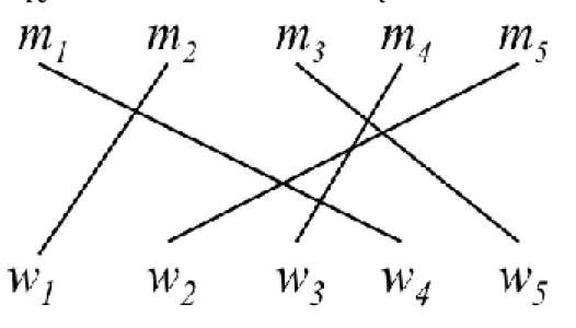
Example 1 Consider the following hierarchical mating economy with 5 men, m1, m2, m3,
m4 and m5, and 5 women, w1, w2, w3, w4 and w5, where the demand for wives by men is
(s1; s2; s3; s4; s5) = (2; 2; 1; 1; 1) and M1 = M (each man may marry). Under monogamy,
the unique equilibrium matching, represented by Figure 1, is the one in which each man mi
matches with woman wi. Under polygyny, in the unique equilibrium matching, represented by
Figure 2, m1 is matched with w1 and w2, m2 is matched with w3 and w4, m3 is matched with
w5, and m4 and m5 are unmatched.
Figure 1: Monogamy equilibrium Figure 2: Polygyny equilibrium
Now, suppose that the demand for wives by men is (s1; s2; s3; s4; s5) = (2; 2; 1; 1; 1) and
M1 = fm1, m2, m3, m4g ( m5 cannot marry). Under monogamy, each man mi will with
woman wi if 1 i 4, and m5 and w5 will be unmatched (Figure 3). Under Polygyny, the
unique equilibrium matching will still be the one represented by Figure 2.
We note that while the number of marriages is the same under monogamy and polygyny in the former economy, the situation is quite di¤erent in the latter economy, where the number of marriages is greater under polygyny than under monogamy. We shall later generalize this result. We also note that in both economies, the monopolizing power of highest-ranked men deprives their lowest-ranked counterparts of wives.
A testable implication of Theorem 1 stated in Corollary 1 below is that the aggregate number of marriages (or nuptiality rate) is higher under a polygynous culture than under a monogamous culture.
Corollary 1 1) The aggregate number of marriages is higher under a polygynous culture than
under a monogamous culture.
2) A woman’s probability of getting married is greater in a polygynous culture than in a monogamous culture.
Proof. 1) Under a monogamous culture, the aggregate number of marriages equals the number
of men who may get married, that is jM1j. Under a polygynous culture, each man mi 2 M1
may have at least one wife. So the aggregate demand for women by men who may get married is at least jM1j. But it follows from the construction of the unique pairwise stable matching
that arises in a polygynous culture in the proof of Theorem 1 that at least jM1j women get
married, which implies that the number of marriages under polygyny is weakly greater than under monogamy. The inequality is strict if si > 1 for some man mi 2 M1.
2) The proof follows from the proof of 1).
Another testable implication of Theorem 1 is that if the maximum number of partners that a man may have is increasing in his social rank, then higher-ranked women (or more beautiful women) have greater chance to enter a polygynous relationship, with the number of co-wives increasing with social rank. This result is summarized in Corollary 2 below.
Corollary 2 If si sj whenever i < j, and if wi and wj are married, then the number of
wives that wi’s husband has weakly exceeds the number of wives that wj’s husband has. The
last inequality may be strict.
Proof. The proof immediately follows from the construction of the pairwise stable matching
in the proof of Theorem 1.
We note that a situation where the number of women that a man may have increases with his social rank is when social rank is measured by wealth and wealth buys women (maybe in the form of bride price). Interestingly, Corollary 2 also implies that more beautiful women are more likely to be cheated upon by their husband. This is because more beautiful women marry wealthier men, who attract other women.
3.2
Beauty is subjective
We consider a variant of a hierarchical mating economy in which men are ranked the same way by the women, but each man has his own ranking of women. The motivation here is that if the desirability of a woman as a partner is based, for instance, on how beautiful she is, each man may have a di¤erent de…nition of beauty. For example, if beauty is determined by height, a man may not want his wife to be much taller than he is. Since men di¤er in height, they rank women di¤erently. We will call it a hierarchical mating economy when all the members of a group have identical preferences over the members of the opposite group. When di¤erentiated preference structures are allowed for members of one group, we will call it a hierarchical mating economy with one-sided subjective rankings.
De…nition 3 A hierarchical mating economy with one-sided subjective rankings is a list E =
(N = M1[ M2[ W; (sj)1 j n; m; ( mw)m2M) where:
sj represents the capacity of individual ij;
m is a linear ordering on M representing the ranking of men by all women, and mw is a
linear ordering on W representing the ranking of women by man m. m also represents
women’s preferences over men’s ranks and m
w represents man m’s preferences over
women’s ranks.
As for hierarchical mating economies, we …nd that a hierarchical mating economy with one-sided subjective rankings has a unique pairwise stable matching. We also give a description of this matching in terms of the number of partners that each individual obtains.
Theorem 2 There exists a unique pairwise stable matching in a hierarchical mating economy
with one-sided subjective rankings. More precisely:
Under a monogamous culture, m1 is matched with "his" highest ranked woman, each
man mi (i = 2; :::; k jM2j) is matched with "his" highest ranked woman (not matched
with mj, j = 1; :::; i 1) if i k jM2j, and all men mi such that i > k jM2j and the
remaining women not matched with any man in M1 are unmatched.
Under a polygynous culture, m1 is matched with "his" s1 = min(s1;jW j) highest ranked
women, m2 is matched with "his" s2 = min(s2;jW j s1) highest ranked women (not
matched with m1), and so on. Iterating, mi is matched with "his" si = min(si;jW j
i 1P
j=1
sj) highest ranked women (not matched with mj, j = 1; :::; i 1), i = 2; :::; k jM2j.
And all men mi such that i > k jM2j and the remaining women are unmatched.
Proof. The reasoning is similar to that of Theorem 1 and so, the proof is left to the reader.
Example 2 Consider the following hierarchical mating economy, analyzed in Example 1, with 5 men, m1, m2, m3, m4 and m5, and 5 women, w1, w2, w3, w4 and w5, where the demand for
wives by men is (s1; s2; s3; s4; s5) = (2; 2; 1; 1; 1) and M1 = M (each man may marry). The
di¤erence is that each man has his own ranking of women. Those rankings are the following: m1 : w4 w1 w2 w3 w5 (that is, m1 prefers w4 over w1, w1 over w2, w2 over w3,
and w3 over w5)
m2 : w1 w3 w2 w4 w5
m3 : w1 w4 w5 w3 w2
m4 : w3 w2 w4 w1 w5
m5 : w2 w1 w3 w4 w5
Under monogamy, the unique equilibrium matching, represented by Figure 4, is the one in which m1 matches with w4, m2 matches with w1, m3 matches with w5, m4 matches with
w3, and m5 matches with w2. Under polygyny, the unique equilibrium matching, represented
by Figure 5, is the one in which m1 matches with w4 and w1, m2 matches with w3 and w2
(his 2 highest ranked women not matched with m1), m3 matches with w5, and m4 and m5 are
Figure 4: Monogamy equilibrium with one-sided subjective rankings
Figure 5: Polygyny equilibrium with one-sided subjective rankings
We remark that the structure of the pairwise stable matching in terms of the distribution of links is the same for the …rst hierarchical mating economy analyzed in Example 1 and the hierarchical mating economy with one-sided subjective rankings being studied under either monogamy (Figure 1 has the same structure as Figure 4) or polygyny (Figure 2 and Figure 5 have the same structure), but the marriages are di¤erent.
As illustrated in Example 2, we note that the unique equilibrium matching which arises in a hierarchical mating economy with one-sided subjective rankings has the same structure as the unique equilibrium matching which arises in the corresponding hierarchical mating economy under either monogamy or polygyny. Both matchings are similar up to permutations of the women, with men having the exact same number of women. This implies that the …nding stated in Corollary 1, according to which the number of marriages is greater under a polygynous culture than under a monogamous culture, holds for hierarchical mating economies with one-sided subjective rankings as well.
3.3
The e¤ect of polygyny on individual-level fertility
In this section, we study the e¤ect of polygyny on fertility at the individual level. We conduct this analysis under two alternative preference structures. First, we assume that children are
the only consumption good in the household.7 Under the second structure, parents derive
utility not only from the number of children they have, but from other goods too. Another salient feature of the second model is that parents have "others’regarding preferences", owing to the fact that the number of children determines the "prestige rank" of parents, so that having more children than other parents generate greater utility.
3.3.1 Children as the only good
Assume that a man m has l wives w1; :::; wl. Each individual derives utility from having
children. A child is conceived out of the consent of his two parents, and is raised with resources contributed by both. For simplicity, we assume that they have identical preferences and endowment. Denote respectively by u and y each individual’s utility function and endowment (endowment includes all types of resources needed to raise a child such as …nancial resources, time, attention, etc.). We assume that u is twice-continuously di¤erentiable and strictly concave and increasing in the number of children. Let c be the price of a child, nm the total
number of children born to the man m and all his wives, and ni the number of children born
to wife wi (i = 1; :::; l). It follows that:
nm = n1+ ::: + nl and cnm = y + ly (1)
Given that a child is conceived out of the consent of his two parents, it makes sense to assume that a man who has several wives decides how many children to give each wife. In fact, a wife cannot have more children than her husband wants to give her. Conversely, a husband cannot give any of his wives more children than the number she desires. But within our framework, we have assumed that man m and each of his wives have identical preferences, so that no wife desires more children than m. We shall therefore consider a unitary household model in which all incomes are pooled together and the husband, acting as a social planner, decides how many children (ni) to give each wife wi. 8 We assume that he allocates children
7This is equivalent to assuming that each parent derives utility from children as well as from other
con-sumption goods, with resources being allocated in a "…xed" proportion between children and these other goods.
8Another way to model the fertility decision of each individual within our context is to assume that the
husband and his wives play a non-cooperative game in which the strategy set of each wife is the set of positive real numbers R+, and the strategy set of the husband is the l cartesian product of the set of positive real
numbers Rl
+ (each wife chooses the number of children she would like to have and the husband chooses the
number of children he would like to have with each wife; and assuming wife i wants to have xichildren and the
husband wants to have xi children with her, then i will have n
i= min(xi; xi) children as the consent of both
the husband and the wife is necessary for a child to be conceived). If we assume that the husband is equally altruistic to his wives in that he cares not only about his own payo¤, but also about the payo¤s of his wives, we can show that the solution of the social planner problem as we model it in this paper is a Nash equilibrium
across his wives so as to maximize a social welfare function such as the following:
U (nm; n1; :::; nl) = u(nm) + u(n1) + ::: + u(nl) 9 (2)
His maximization problem can be formulated as follows:
M aximize U (nm; n1; :::; nl) = u(nm) + u(n1) + ::: + u(nl)
subject to nm = n1+ ::: + nl; (3)
cnm = y + ly;
ni 0; i = 1; :::; l
It is easy to see that the solution of (3) is the egalitarian solution ni = nw = y
lc +
y
c for
all i = 1; :::; l and nm = y+lyc .10 Interestingly, we note that the functional form of n
w shows
that each woman receives the number of children corresponding to her own endowment plus her husband’s endowment shared equally across all wives. These results lead to the following testable implications, which say that the number of children that a man has increases with the number of wives he has, but the number of children that each wife has decreases with the number of co-wives.
Proposition 1 nm is strictly increasing in l and nw is strictly decreasing in l.
Proof. The proof comes from the expression of nm and nw above.
We note that Proposition 1 implies that a woman in a monogamous relationship has more children than a woman in a polygynous relationship. However, a man in a monogamous relationship has less children than a man in a polygynous relationship.
3.3.2 Envy or children as a signal of prestige
We now introduce envy or "others’regarding preferences" in the model. This may arise in a context in which the number of children is a source of prestige to their parents, so that having
of the fertility game we just de…ned. In addition, that Nash equilibrium can be shown to be e¢ cient. It follows that our social planner model is a realistic model of fertility decisions within our framework.
9Note that our social welfare function is slightly di¤erent from traditional social welfare functions which
do not incorporate the social planner’s utility. In this respect, our social planner is not entirely "benevolent".
10The egalitarian solution arises because we assume that the husband marries all his wives simultaneously,
or that the order in each he marries his wives is random. We could have assumed a sequential model in which the husband marries his wives in a …xed order as follows: he marries woman 1 in the …rst period, woman 2 in the second period, and so on, until he marries all his l wives. In each period t, the husband solves problem (3), maximizing the social welfare function U (nm; n1; :::; nt) = u(nm) + u(n1) + ::: + u(nt) under the assumption
that his endowment y is equally split across the l periods in which he marries. The number of children that each wife produces after the l periods is the sum of children produced since marrying the husband. Solving this problem shows that higher-order wives will have more children, but the number of children that the husband will have will not di¤er from the number of children produced under the assumption that he marries his wives simultaneously. It follows that the relationship between polygyny and the "average" number of children for each woman is the same whether we assume a simultaneous model or a sequential model.
more children than other parents in the society generates more utility. More formally, if we let nij be the number of children born to an individual ij 2 N, and n m be the total number
of children born to his/her neighbor, then the individual’s utility is increasing in nij n m
where > 0 is the degree to which he/she envies his/her neighbor. In particular, if tends
to 0, there is little envy, a situation similar to our assumption in Section 3.3.1. We shall also assume that each individual derives utility from other consumption goods that we summarize into a single variable x 2 R+. It follows that each individual’s utility function is de…ned
over the collection of bundles (nij n m; x). For simplicity, we shall assume such a utility
function to be additively separable, so that it can be written as:
u(nij n m) + v(x) (4)
where each of the functions u and v is twice-continuously di¤erentiable, strictly concave and increasing.
Following the same argument developed in the model without envy, we shall consider a unitary household model again where the husband, acting as a social planner, allocates children across his wives and the x good across his wives and himself. If we let p be the price of the x good, his maximization problem will now be:
M aximize U (nm; n1; :::; nl; xm; x1; :::; xl) = u(nm n m) + v(xm) + u(n1 n m)
+v(x1) + ::: + u(nl n m) + v(xl)
subject to nm = n1+ ::: + nl; (5)
cnm+ p(xm+ x1+ ::: + xl) = y + ly;
ni 0; i = 1; :::; l;
xm 0; xi 0; i = 1; :::; l
The following claims will be useful in the analysis of this maximization problem.
Claim 1 U attains a maximum in the constraint set.
Proof. It follows from the constraints that each ni 2 [0;y+lyc ] and each xi 2 [0;y+lyp ], i =
m; 1; 2; :::; l. The constraint set therefore is C = [0;y+lyc ]l+1 [0;y+ly
p ]
l+1, which is a closed and
bounded subset of R2(l+1). Hence, it follows from the Heine-Borel Theorem that C is compact.
Given that U is a real-valued continuous function de…ned on a compact set, we conclude by the Bolzano-Weierstrass Theorem on the existence of extreme value that U attains a maximum in C.
Claim 2 Let f be a real-valued continuous function de…ned on a bounded interval I R. If f
is strictly concave and increasing, then the function de…ned by g(x1; :::; xn) = f (x1)+:::+f (xn)
Proof. The proof is left to the reader.
Given that U is additively separable, following Bergstrom (2011), (4) can be split up into the following maximization problems:
M aximize u(nm n m)
subject to cnm = y1 (6)
and
M aximize u(n1 n m) + ::: + u(nl n m)
subject to nm = n1+ ::: + nl; (7) ni 0; i = 1; :::; l and M aximize v(xm) + v(x1) + ::: + v(xl) subject to p(xm+ x1+ ::: + xl) = y2; (8) xm 0; xi 0; i = 1; :::; l
where y1 + y2 = y + ly. Here, income is spent on children (y1) and other consumption
goods (y2). But unlike in Section 3.3.1, the allocation of income between these two types of
goods is not …xed.
The solution of (6) is nm = y1
c. It follows from Claim 2 that the solution of (7) is (n1; :::; nl)
such that n1 = n2 = ::: = nl = nm
l , and the solution of (8) is (xm; x1; :::; xl) such that
xm = x1 = ::: = xl
Since the egalitarian solution arises in equilibrium, suppose ni = nw (i = 1; :::; l), and
xi = x (i = m; 1; :::; l). Our maximization problem then becomes:
M aximize U (nw; x) = u(lnw n m) + lu(nw n m) + (l + 1)v(x)
subject to clnw+ p(l + 1)x = y + ly (9)
nw 0
x 0
Claim 1 and Claim 2 ensure that a unique equilibrium exists. We distinguish three cases: (a) nw = 0; (b) x = 0; (c) nw > 0 and x > 0.
If nw = 0, then x = p(l+1)y+ly . If x = 0, then nw = y+ly
cl , which corresponds to the previously
analyzed situation in which children were the only good.
implies that the social planner’s problem will simply consist of maximizing: U (nw) = u(lnw n m) + lu(nw n m) + (l + 1)v( y + ly clnw p(l + 1) ) (10) or equivalently U (nm) = u(nm n m) + lu( nm l n m) + (l + 1)v( y + ly cnm p(l + 1) ) (11)
Both functions will be useful for the comparative statics analysis. The …rst order conditions for these two functions are respectively:
U0(nw) = lu0(lnw n m) + lu0(nw n m) cl pv 0(y + ly clnw p(l + 1) ) = 0 (12) and U0(nm) = u0(nm n m) + u0( nm l n m) c pv 0(y + ly cnm p(l + 1) ) = 0 (13)
We derive testable implications. First, the number of children that a man has increases with the number of his wives, but the number of children that each wife has increases or decreases with the number of wives depending on the utility function.
Proposition 2 nm is strictly increasing in l. nw may be strictly increasing or decreasing in
l depending on the utility function.
Proof. 1) We want to show that at nm = nm, @n@lm > 0. First compute
@nm
@l by applying the
Implicit Function Theorem to (13). Write:
U0(nm) = u0(nm n m) + u0(nml n m) cpv0(y+ly cnp(l+1)m) = f (nm; l; n m). We have: @nm @l = @f (nm;l;n m) @l ( @f (nm;l;n m) @nm ) 1.
The reader can check that:
@f (nm;l;n m) @l = ( nm l2 u00( nm l n m) c 2n mv00((l+1)y cnp(l+1) m)). It follows that @f (nm;l;n m)
@l < 0 given that u00< 0 and v00< 0 by assumption.
Also, we have: @f (nm;l;n m) @nm = u 00(n m n m) + 1lu00(nlm n m) + c 2 p2(l+1)v00( (l+1)y cnm p(l+1) ) < 0.
This implies that (@f (nm;l;n m)
@nm )
1 < 0. Since @nm
@l is the product of two negative numbers,
it is positive.
2) Let us prove that at nw = nw, the sign of @n@lw is ambiguous. Compute
@nw
@l by applying
the Implicit Function Theorem to (12). Write: U0(n w) = lu0(lnw n m) + lu0(nw n m) clpv0(y+ly clnp(l+1)w) = g(nw; l; n m). We have: @nw @l = @g(nw;l;n m) @l ( @g(nw;l;n m) @nw ) 1.
The reader can check that: @g(nw;l;n m) @l = (lnwu00(lnw n m)+u0(lnw n m)+u0(nw n m) c pv0( (l+1)y clnw p(l+1) ) c2ln w p2(l+1)2v00( (l+1)y clnw p(l+1) )).
Given that u0 > 0 and u00 < 0, the sign of @g(nw;l;n m)
@l is clearly ambiguous. It could be
positive or negative. However, we have the following:
@g(nw;l;n m) @nw = (l 2u00(ln w n m) + lu00(nw n m) +p2(l+1)cl v00( (l+1)y clnw p(l+1) ) < 0. So if @g(nw;l;n m) @l > 0, then @nw @l < 0, and if @g(nw;l;n m) @l < 0, then @nw @l > 0.
We also analyze the impact of a neighbor’s fertility on an individual’s own fertility. We …nd that an individual’s number of children is positively a¤ected by the number of children his neighbor has, which is a contagion e¤ect of fertility.
Proposition 3 nm is strictly increasing in n m.
Proof. It su¢ ces to prove that @nm
@n m > 0. First write Equation (13) as:
U0(n
m) = u0(nm n m) + u0(nlm n m) pcv0(y+ly cnp(l+1)m) = f (nm; l; n m).
Apply to this equation the Implicit Function Theorem. We have:
@nm @n m = @f (nm;l;n m) @n m ( @f (nm;l;n m) @nm ) 1.
The reader can check that:
@f (nm;l;n m) @n m = [( u 00(n m n m) u00(nml n m)] < 0. Also, we have: @f (nm;l;n m) @nm = u 00(n m n m) +1lu00(nml n m) + c 2 p2(l+1)v00( (l+1)y cnm p(l+1) ) < 0. It follows that (@f (nm;l;n m) @nm ) 1 < 0. We conclude that @nm @n m > 0, which holds at nm = nm.
Not surprisingly, we note from the expression of @f (nm;l;n m)
@n m in the proof that as the
degree of envy ( ) tends to 0, the marginal e¤ect of an individual’s neighbor fertility on his own fertility tends to 0 as well. So fertility is only as contagious as envy is strong.
As a corollary of Proposition 3, a monogamous individual in a functioning polygynous culture has more children than a monogamous individual in a monogamous culture.
Corollary 3 Any individual, regardless of whether he/she is involved in a monogamous or a
polygynous relationship, has more children if he/she lives in a functioning polygynous culture than if he/she lives in a monogamous culture.
Proof. The proof follows from the fact that in a functioning polygynous culture, there is at
least one man who has several wives, and who by Proposition 2 has more children than he would have had in a monogamous culture. An individual in a polygynous culture is therefore exposed to the fertility behavior of such a polygynist, which by Proposition 3 has a positive e¤ect on his/her own fertility.
3.4
Aggregate fertility in a polygynous versus a monogamous
cul-ture
In this section, we investigate the e¤ect of matrimonial culture on the total number of children in a society. Our analysis draws on the …ndings of the previous sections. We will distinguish two situations, namely one in which the number of children that a woman has decreases with the number of wives her husband has, and one in which the opposite holds. From the analysis conducted in previous sections, we know that the …rst situation occurs when children are the only consumption good, or under certain conditions, when children bring prestige to their parents. We will see that in such a situation, the e¤ect of a polygynous culture on the aggregate number of children is ambiguous.
Let (si)i2M be the demand for women by the men in a hierarchical mating economy. We
know that M = M1[ M2 and si = 0 if i 2 M2. We have the following result.
Proposition 4 Assume that @nw
@l < 0.
1) If P
i2M1
si < jW j, then the total number of children is greater in a polygynous culture than in a monogamous culture. The inequality is strict if si > 1 for some man mi 2 M1.
2) If P
i2M1
si jW j, then the total number of children may be lower in a polygynous culture than in a monogamous culture.
Proof. 1) If P
i2M1
si <jW j, meaning that the aggregate demand for women by the men who
may get married is smaller than the total number of women, then obviously, each man in M1
will obtain his optimal number of women in the unique equilibrium that exists in the economy.
Since each man in M1 has at least one woman, by Propositions 1 and 2, each such man will
have at least the number of children he would have had in a monogamous culture, implying that the total number of children is greater in a polygynous than in a monogamous culture. Assume that si > 1 for some man mi 2 M1. By Propositions 1 and 2, given that mi has more
than one wife, he will have strictly more children than he would have had in a monogamous culture, which implies strict inequality when we compare the aggregate number of children under the two regimes.
2) If P
i2M1
si jW j, all women will get married in a polygynous culture, but some men in
M1may remain unmatched. Let us show by a simple example that the total number of children
may be lower in a polygynous culture than in a monogamous culture. Consider a hierarchical mating economy that has 4 men m1, m2, m3, and m4 and 4 women w1, w2, w3, and w4, where
(s1; s2; s3; s4) = (2; 2; 1; 1) and M1 = M (each man may marry). Suppose that preferences
for the number of children are such that a monogamous man gets 3 children and a man who has two wives gets 4 children, with each wife having 2 children (note that this assumption is consistent with @nm
@l < 0). Under monogamy, the unique equilibrium matching is the one in
thus the total number of children is 12. Under polygyny, the unique equilibrium matching is one in which m1 is matched with w1 and w2, m2 is matched with w3 and w4, and m3 and m4
are unmatched. In this case, m1 and m2 will have 4 children each, and m3 and m4 will have
no children, yielding a total of 8 children. We conclude that in this particular example, the total number of children is smaller under polygyny than under monogamy, despite the fact that a polygynist has strictly more children than a monogamist at the individual level. Note, however, that if (s1; s2; s3; s4) were (2; 1; 1; 0), the other assumptions remaining unchanged, the total number of children would have been 10 under polygyny and 9 under monogamy, and the conclusion therefore would have been di¤erent.
We note that the condition under which polygyny positively a¤ects aggregate fertility is more likely to be empirically valid, as there exist single women even when polygyny is allowed. In the second situation where the number of children that a woman has increases with the number of wives her husband has, we …nd that the total number of children is greater in a polygynous culture than in a monogamous culture.
Proposition 5 Assume that @nw
@l > 0. Then, the total number of children is greater in a
polygynous culture than in a monogamous culture. The inequality is strict if si > 1 for some
man mi 2 M1.
Proof. By Corollary 1, we know that the number of women who get married is greater in a
polygynous than in a monogamous culture. Since @nw
@l > 0 by assumption, under polygyny,
each such woman has at least the number of children she would have got under monogamy, which implies that the total number of children is greater in a polygynous than in a monoga-mous culture. If one such woman shares her husband with at least one woman (that is, si > 1 for some man mi 2 M1), by the assumption that @n@lw > 0, she will have strictly more children
than she would have had in a monogamous culture, which yields the strict inequality.
4
Testable and tested predictions
The model developed in the preceding sections has yielded a rich set of testable predictions that we summarize below:
1. Beautiful women are more likely to be married (this follows from Theorem 1).
2. Beautiful women are more likely to be married to polygynous men, or to be cheated if polygyny is not allowed (Corollary 2).
3. Beautiful women are more likely to have at least one child–the extensive margin–(this follows immediately from the fact that (a) female beauty increases marital success as implied by Theorem 1, and (b) the demand from children is greater within marriage).
4. Beauty has no clear e¤ect on the number of children produced by a woman–the intensive margin– as female beauty increases the likelihood of marrying a polygynist, but being married to a polygynist has an ambiguous e¤ect on the number of children produced (see prediction 8 below).
5. Higher-status men are more likely to be polygynous (Theorem 1, Theorem 2). 6. Polygyny prevalence increases the likelihood of marriage for women (Corollary 1). 7. A polygynous man has more children than a monogamous man (Proposition 1,
Propo-sition 2).
8. Being married to a polygynous man has an ambiguous e¤ect on the number of children produced by a woman: the e¤ect may be negative or positive, or there might be no e¤ect (Proposition 2).
9. Women, regardless of whether they are involved in a monogamous or polygynous rela-tionship, have more children as the prevalence of polygyny in their region of residence increases, which is the contagious e¤ect of polygyny on fertility (Corollary 3).
10. Polygyny prevalence has a positive e¤ect on aggregate fertility (Proposition 4, Proposi-tion 5). According to proposiProposi-tion 4, the e¤ect may be negative if the aggregate demand for women is greater than the supply of women, something that is usually not observed in reality.
Our testable predictions can be divided into two sets. The …rst set ((1)-(5)) reveals the e¤ect of female and male characteristics such as beauty and wealth on marital and reproductive outcomes. The second set ((6)-(10)) reveals the multi-faceted e¤ects of polygyny and polygyny prevalence on individual and aggregate fertility.
Clearly, these predictions are too many to be rigorously tested in only one paper. We therefore only focus our e¤orts on a limited number of predictions, which are those that have not been su¢ ciently tested in the literature. Also, because of data limitations, we will only be able to perform a descriptive analysis for most of the tested predictions, showing only cor-relations. In the …rst part of the empirical section, we will test the e¤ect of female beauty on marital and reproductive outcomes ((1)-(4)). The second part will test the micro-level mech-anism through which polygyny prevalence positively a¤ects aggregate fertility. According to the theory, polygyny prevalence increases aggregate fertility throught two main channels: (1) by increasing the number of marriages (prediction 6); and (2) by trigerring fertility contagion (prediction 9). Because our study is the …rst to theoretically document this second channel through which polygyny prevalence a¤ects fertility, we will also try to empirically establish its causality. All these tests will be carried out using household data from multiple sub-Saharan African countries.
5
Empirical test of the model
5.1
Data
The data is taken from the DHS surveys and covers 32 countries from sub-Saharan Africa.11
As marriage and fertility outcomes both vary with time and age, we use several waves of surveys for each country whenever possible (see Appendix Table A) to disentangle those two dimensions.12
Polygyny is only illegal in six countries13. But legal changes in polygyny regulations can
hardly be considered as exogenous events. They tend to follow the evolutions of customs rather than the contrary. Indeed several countries encountered severe di¢ culties in passing laws to
ban polygyny (for instance, Uganda) or in enforcing them (Senegal).14 Moreover, polygyny
is common, although less widespread, in countries where it is unlawful, such as Burundi or Madagascar.
Table 1 presents average statistics over countries in our sample. First, at around three children born per woman, ranging from 3.9 in Niger to 1.9 in South Africa, average fertility remains high throughout the continent.
The percentage of women involved in a relationship, either through a legal union or an informal cohabition, is also rather elevated, ranging from 38% in Namibia to 86% in Niger.
Polygyny appears to be very frequent, and is more widespread in western Africa than elsewhere on the continent. 43% and 45% of women in Senegal and Benin respectively, are married to polygynous men, versus less than 20% in Eastern Africa.
Interestingly, the desire for children is acknowledged to be very high, with many women still giving unrealistic answers to the question regarding the ideal number of children they would like to have. On average, women declare wanting more than seven children, but this number even exceeds ten in six countries. In spite of a declining fertility, preferences for children remain strong.
11The Demographic and Health Survey (DHS) used in this study were carried out by : the Statistical and
Health Services (Ghana), the Institut National de la Statistique (Cote d’Ivoire), the Institut National de la Statistique (Benin), the Ministère du Plan et de l’Aménagement du Territoire (Cameroon, 1991), the Bureau Central des Recensements et Etudes de Population (Cameroon, 1998), the Institut National de la Statistique (Cameroon, 2004), the Centre National de Recherches sur l’Environment (Madagascar, 1992), the Institut National de la Statistique (Madagscar, 1997, 2003, 2008), the National Statistical O¢ ce (Malawi), the Federal O¢ ce of Statistics (Nigeria, 1990), the National Population Commission (Nigeria, 1999, 2003, 2008), the O¢ ce National de la Population (Rwanda, 1992, 2000), the Ministry of Economics (Rwanda, 2005), the Ministère des Finances (Senegal, 1992, 1997), the SERDHA (Senegal, 1999), the Ministère de la Santé, CRDH (Senegal, 2005, 2006), the National Bureau of Statistics (Tanzania), the Bureau of Statistics (Uganda) and the Central Statistical O¢ ce (Zimbabwe).
12There are 25 countries with more than one survey available and 19 with at least three surveys. 13See annex A for details.
14In Senegal, as in many other countries, men are supposed to choose a “polygynous” or “monogamous”
status when they marry for the …rst time. However, it is common for men who opted for monogamy during their youth to later marry a second wife. This law is di¢ cult to enforce as the …rst spouse may have to choose between polygyny and a divorce.
Female education is low, as many women surveyed between the ages of 15 and 49 did not bene…t from the push toward universal primary education of the early 2000s. Average years of schooling exceeds six years in only six out of 32 countries. Finally, infant mortality rates are still very high, ranging from 37 per thousand in Zimbabwe to 85 per thousand in Mozambique.
[Table 1]
5.2
Beauty, marriage, polygyny, and fertility
We test the propositions that more beautiful women are more likely: (i) to be married (pre-diction 1); (ii) to be married to polygynists (pre(pre-diction 2); and (iii) to have at least to have at least one child (prediction 3). We also test the e¤ect of beauty on number of children conditional on fecundity (prediction 4). Prior to testing these relationships, it is appropriate to discuss how beauty is measured.
5.2.1 Measuring beauty
The physical attractiveness of women is an important factor in determining their desirability as partners. As explained by Pawlowski (2003), sexual selection is a well established evolutionary process based on preferences for speci…c traits in one sex by members of the other sex. It is important in the evolution of morphological traits, and several sexually dimorphic traits in humans, such as facial hair and facial shape. In general, however, the appreciation of beauty varies across the world. Some components of external beauty such as low waist-to-hip ratio (Singh, 1995) and clear complexion (Symons, 1979) are agreed upon across most cultures. However, other attributes such as weight and skin tone vary across cultures and time frames. In renaissance art, most women are depicted as large women with pale skin. Both of those features were indicators of wealth and good health. In contrast, most of the women displayed in media as symbols of beauty today are thin and have tanned skin.
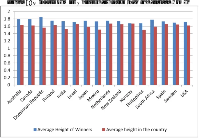
In present day "media", height and thinness are the standard for beauty. Models across the world are much taller than average. While walking the runway, heights are exaggerated even further with high heels. Most mannequins displaying women’s attire in stores tower over customers and beauty pageants are dominated by tall and thin women. One of the biggest international beauty contests is Miss Universe, where beauty contest winners from several countries compete for the international title. We calculate that the average height of the titleholders from 1980-2011 is 1.75 m, and …nd that all the winners are taller than the average women of their nationality (see Figure 6 for selected countries). As people are widely exposed to and in‡uenced by media today, taller women are regarded as more beautiful and in turn more desirable.
Figure 6: Winners of Miss Universe are taller than the average women
It follows that several measures of beauty, including waist-to-hip ratio, skin complexion, height, weight, body mass index (calculated as weight in kilograms divided by the square of height in meters), have been used in the literature.15 Of these measures, height, weight and the BMI are the most popular, perhaps because of their availability in most datasets (e.g., Chiappori, Ore¢ ce, and Quintana-Domeque 2012). The DHS data used for our analysis have information on these anthropometric indicators. Therefore, we use all the three indicators as proxies for beauty. However, only height appears to produce results that are consistent with our model. In fact, due to the cross-sectional nature of the DHS datasets, height is a more appropriate, although imperfect, measure of physical attractiveness because it is more stable over time than weight and BMI after a certain age. Indeed, since our goal is partly to study the e¤ect of beauty on marriage outcomes, weight and BMI measured at the survey are not appropriate measures of beauty because the weight and BMI of a woman who is married at the survey may be very di¤erent than when she got married, and will therefore fail to explain her "past" marriage outcome. But such a woman most likely has the same height as when she got married, and so, "current" height as a measure of beauty can explain her "past" marriage outcome. The other advantage of using height is that it is determined by genetic, feotal and early childhood conditions (Martorell and Habicht 1986; Schultz 2002; Eveleth and Tanner 1976), and so should largely be viewed as preceding or being exogenous to the marital and
15Importantly, the multiplicity of measures seems to indicate that there is no perfect measure for beauty.