HAL Id: halshs-00662513
https://halshs.archives-ouvertes.fr/halshs-00662513v3
Preprint submitted on 22 Jul 2016
HAL is a multi-disciplinary open access
archive for the deposit and dissemination of sci-entific research documents, whether they are pub-lished or not. The documents may come from teaching and research institutions in France or abroad, or from public or private research centers.
L’archive ouverte pluridisciplinaire HAL, est destinée au dépôt et à la diffusion de documents scientifiques de niveau recherche, publiés ou non, émanant des établissements d’enseignement et de recherche français ou étrangers, des laboratoires publics ou privés.
Contagion in financial networks: a threat index
Gabrielle Demange
To cite this version:
WORKING PAPER N° 2012 – 02
Contagion in financial networks: A threat index
Gabrielle Demange
JEL Codes: G01, G21, G28
Keywords: contagion of default, financial linkages, intervention policy
P
ARIS-
JOURDANS
CIENCESE
CONOMIQUES48, BD JOURDAN – E.N.S. – 75014 PARIS TÉL. : 33(0) 1 43 13 63 00 – FAX : 33 (0) 1 43 13 63 10
www.pse.ens.fr
CENTRE NATIONAL DE LA RECHERCHE SCIENTIFIQUE – ECOLE DES HAUTES ETUDES EN SCIENCES SOCIALES
Contagion in financial networks: A threat index
Gabrielle Demange*forthcoming in Management Science July 19, 2016
Abstract This paper proposes to measure the spill-over effects that cross-liabilities generate on
the magnitude of default in a system of financially linked institutions. Based on a simple model and an explicit criterion -the aggregate debt repayments- the measure is defined for each
institu-tion, affected by its characteristics and links to others. These measures -one for each institution-summarize relevant information on the interaction between the liabilities structure and the shocks
to resources and they can be useful to determine optimal intervention policies. The approach is illustrated to evaluate the consolidated foreign claims of 10 EU countries.
Keywords : contagion of default, financial linkages, intervention policy JEL G01, G21, G28
1
Introduction
An intricate web of claims and obligations ties together the balance sheets of a wide variety of insti-tutions, especially in the financial sector between banks, hedge funds, and various intermediaries.
Some argue that these ties have played a large role in the dissemination of the financial crisis of 2007-2008. As such, cross-liabilities are an important concern for both the financial institutions
and the regulators and there is a general call for addressing their role in the risk of the system, the so-called 'systemic' risk.1 This paper proposes to measure the spill-over effects that cross-liabilities
generate on the magnitude of default in a system of financially linked entities. Based on an explicit criterion -the aggregate debt repayments- the measure is defined for each institution, affected by its
characteristics and links to others. These measures -one for each institution- summarize relevant information on the interaction between the liabilities structure and the shocks to resources. They can be useful to a regulator to determine how to inject cash during a liquidity crisis, to the safe
1
The new framework proposed by the Basel committee (Basel III) identifies some 'systemically important financial institutions' (SIFI) from which higher standards are required. The SIFI are mainly determined by their size.
institutions to decide which debts they should write-off in priority, or to evaluate the impact of rais-ing capital before the occurrence of default. The approach is illustrated on the consolidated foreign claims of 10 EU countries.
The risk considered in this paper comes from the default of institutions on their cross-liabilities, as occurs during liquidity crises. The capacity of an institution to repay its liabilities depends not
only on its revenues from outside activities -its operating cash-flow- but also on the reimbursements on its claims, calling for a joint determination of the repayments that reflects the full extent of the
propagation of defaults. In this paper, repayments are endogenous, determined by the clearing mechanism due to Eisenberg and Noe (2001) (hereafter EN). At clearing repayment ratios, each
institution in default reimburses as much as it can given others' repayments and limited liability.2 The aggregate repayments are thus endogenously determined as a function of the cash-flows of all
institutions.
The impact of an institution on the system is measured by the variation in these aggregate
repayments following a decrease in the cash-flow of the institution. When the institution does not default, the variation is null. When it defaults, the variation includes not only the decrease in its
repayment following the decrease in its cash-flow but also the decrease caused by the propagation of defaults, the spill-over effects. The variation is simple to compute if the institution's cash-flow
decrease is moderate enough to leave unchanged the set of defaulting institutions. In that case, the variation is proportional to a term called hereafter threat index. The index of defaulting i counts
all the chains of successive defaulting creditors starting at i, discounted by liabilities' proportions.3 This implies that the threat indices of defaulting institutions depend on the financial health of their
(direct and indirect) creditors. Since repayment ratios depend on the health of their debtors, threat indices and repayment ratios may not be aligned.
The default of an institution is interpreted here as temporary, not as bankruptcy.4 For example, creditors agree to postpone unpaid debts, as within the network of firms described in Kiyotaki and
Moore (1997).5 In the financial sector, this situation corresponds to an illiquidity episode, in which all institutions are solvent (and it is commonly known) but possibly default due to liquidity
con-straints. The clearing mechanism organizes these delays in an orderly way, thereby avoiding costly liquidation of projects or run phenomena. Though temporary, defaults have an impact when
activ-2Limited liability can also interpreted as a liquidity constraint, see Section 3. 3
It is thus given by a centrality 'Katz-Bonacich' index on the network of defaulting banks (see the related literature).
4
Alternatively, if we assume as Elliott et al. (2013) that an institution is bankrupt when its ratio falls below a threshold, the analysis applies to the situations where the cash-flows are large enough so that each ratio is above the threshold.
5In their model, firms are symmetric and the shocks are macro-economic, affecting all cash-flows identically. The
ities are linked to the total reimbursed amounts (as developed in a two-period model in Section 3). In such a case, the intervention of a regulator or a change in the institutions' agreements to improve the reimbursement flows are justified.
The analysis has several policy implications. First, an injection of cash, by increasing institu-tions' cash-flows, results in an increase in the activity. To obtain the maximal improvement, the
injection must account for the spill-over effects across institutions. When the amount of cash is moderate, the optimal policy is characterized by the threat indices: Cash should be injected into the
defaulting institutions with the largest threat index, which are not necessarily those with the lowest repayment ratio. Similarly, the optimal policy of postponing or writing-off part of the claims of the
safe institutions on the defaulting ones is determined by the threat indices.
Second, the lack of information on the bilateral liabilities between financial institutions is a
concern to regulators. How valuable is this information? To address this question, I compare the optimal injection strategy, which assumes complete information, with the benchmark in which
the regulator knows the total liabilities and claims of each institution but not the bilateral ones. The value of information is defined as the improvement in the aggregate repayments reached by
the optimal policy under complete information over the benchmark. When the injected amount is moderate, the value is proportional to the difference between the maximal threat index and its
average over the defaulting institutions. This difference, hence the value of information, is driven by the asymmetry in the liabilities' proportions of the defaulting institutions to each other.
Third, the impact of increasing capital levels can be assessed by considering an ex ante stage before the cash-flows are realized and the clearing ratios are determined. The value of raising the
capital of an institution at the margin is the expectation of its threat index. The value is increasing in both the institution's default probability and the expected spill-over effects conditional on its default.
The latter are increasing in the (random) size of the defaulting set when the institution defaults. Even if cash-flows are independent, the cross-liabilities induce positive correlations between defaults,
which in turn increase the conditional spill-over effects hence the values of raising the capital. Also, the size of an institution has an ambiguous effect on the value of raising its capital, reflecting
the two roles a large institution may have: on one hand, its large reimbursements serve as a cushion to its defaulting creditors when it does not default, on the other, its default causes more defaults.
Finally, to illustrate the approach, I use consolidated foreign claims between 10 EU countries6 and compute expected ratios and threat indices. The results uncover interesting features that are not
6The data is available from the Bank of International Settlements. The same data on 6 EU countries is used by Elliott
easy to detect from the liabilities structure because of its asymmetry and heterogeneity.
The literature on financial contagion is growing very fast. It investigates various channels of contagion and spill-over effects in a financial system, through the cross-liabilities as here, or through
correlation in cash-flows, fire sales, panic phenomena amplified by asymmetric information and mis-coordination. I review the most related works to this paper.
Empirical studies have examined the potential for contagion in calibrated interbank markets, as reviewed by Upper (2011). Recent studies, often based on simulations, aim to assess the impact of
cross-holdings on contagion7(Nier et al. 2007, Gai and Kapadia 2010, Elliott et al. 2013, Glasser-man and Young 2015, Acemoglu et al. 2015) and to identify the strength of the risk-sharing versus
risk-spreading effects of the liabilities. These works measure the risk of the system by the expected contagion size (say, the expected number of defaulting banks) triggered by a bank picked at
ran-dom. Given the observed heterogeneity of financial institutions, both in their size and connections, it is important to assess the spill-over effects initiated by a given institution, as is performed by the
measure introduced in this paper.
Several approaches have been followed to measure the risk of a particular institution while
accounting for the interdependencies within the system. Most of the proposals consider the inter-dependencies induced by correlated portfolios and amplification phenomena due to fire sales and
neglect the impact of the cross-liabilities. One approach extends the standard banks' risk indicators -VaR, expected shortfall- by conditioning on systemic events, which are defined as those where a
stock index falls below a threshold (the CoVaR measure in Adrian and Brunnermeier 2011 and the Marginal Expected shortfall in Acharya et al. 2011 or Brownee and Engle 2010). These measures
are based on a reduced form and cannot distinguish between the initiation and contagion effects. An alternative approach takes the perspective of the management of the risk in a banking system.
Viewing a regulator as owning a portfolio (composed of short put options) on banks due to its role as a lender of last resort, Lehar (2005) assesses the risk of that portfolio and the contribution of
each bank to that risk. My approach is similar in the sense that the impact of an institution on the system is defined in reference to an aggregate indicator, the aggregate repayments. Greenwood
et al. (2015) assess the vulnerability of banks in a model where the channel of contagion comes from fire sales induced by active asset management. Incorporating the two channels of contagion,
cross-liabilities as here and fire sales, would give a threat index that would depend not only on the liabilities structure but also on the similarity in holdings and the sensitivity of prices to sales.
Gouriéroux et al. (2012), based on the equilibrium EN model, consider the impact of a shock, say in
7
stock prices, on the equilibrium and the number of defaults, thus with a different criteria than here. Finally, Cont et al. (2010) define the `contagion' index of a bank as the expected loss in all banks' tier 1 capital induced by the bankruptcy of that bank and estimate these indices on the Brazilian
interbank network. The default mechanism differs from here since defaulting banks are bankrupt and inflict losses to their creditors defined by an exogenous and small recovery rate; instead in this
paper, default is gradual and temporary.
The intervention policies considered here are adapted to liquidity crises encountered by solvent
institutions. Other policies have been investigated in the context of bankruptcy, when the default of an institution involves additional costs. An important issue is then to identify conditions under
which the institution should be bailed out. Rogers and Veraart (2013) consider the incentive for the stockholders of a pool of banks to rescue a failing bank. Building on that model, Alter et
al. (2014) estimate the impact of different rules of reallocation of capital on a measure of bankruptcy losses in the German interbank market. Though the externalities differ from here, they find that
capital rules based on Katz-Bonacich centrality indices perform better than other measures. Another intervention policy investigated recently is to help the strongest banks by providing them liquidity
under a financial crisis. Such a policy can been justified in order to limit fire sales from the solvent but illiquid ones (Diamond and Rajan 2011), to help them buy the assets of bankrupt banks (Acharya
and Yorulmazer 2008) or to limit panic phenomena (Choi 2014).
Finally, the paper relates to the large literature that studies the interactions and externalities
channeled through a network of connections. Firstly, the threat index provides an assessment of a position in a network, and, as such, is related to the power or centrality indices introduced in the
sociological literature by Katz (1953) or Bonacich (1987). These indices depend on an `attenuation' parameter that captures the importance of indirect links. The approach here differs in an important
way since it is based on an explicit criterion. As a result, both the relevant network (the sub-network of the defaulting institutions) and the importance of indirect links are endogenous. Secondly,
inter-vention policies have been investigated in games in which individual actions generate externalities channelled through a network. In a criminal network for example, the 'key player' to remove, the
one whose arrest triggers the largest decrease in global criminal activity, may not be the most ac-tive one (see Ballester et al. 2005). A similar result holds in our model since the most threatening
institutions are not necessarily those with the lowest repayment ratios.
The paper is organized as follows. Section 2 presents the model and the EN clearing mechanism,
analyzes how the aggregate repayments vary with the cash-flows, and defines the threat indices. Section 3 examines intervention policies -cash injection and writing-off of claims-, and computes
the value of the information on the cross-liabilities. Section 4 takes an ex ante point of view and introduces the value of raising capital. Section 5 illustrates the approach on the consolidated foreign claims for 10 EU countries and Section 6 concludes. Section 7 gathers the proofs.
2
A model with defaults
There are n institutions in a financially linked system, say banks, hedge funds, and various inter-mediaries in a financial system, or countries in an integrated market as considered in Section 5.
Denote N = {1, · · · , n}. Institutions hold claims on each other that arrive at maturity and have the same priority. The liability of i towards j is denoted by ℓij. Institutions are endowed with a
positive amount of resources to honor these debts, their operating cash-flow, denoted by zi for i.
The n-vector z = (zi) and the n× n matrix ℓ = (ℓij) where ℓiiis null for each i summarize the
relevant data.
No assumption is made on ℓ as the liabilities' pattern depends on the situation under
considera-tion. In payment systems, liabilities are often both ways, reflecting common clienteles for example. In long term arrangements, some patterns are more directed, such as the ones described in the
Aus-trian banking system, with almost a pyramidal structure (see for example Upper and Worms 2004). The next section describes the EN mechanism by which the claims are liquidated and Section 2.2
analyzes how the aggregate payments vary with the cash-flows.
2.1 The clearing mechanism
Claims are liquidated according to the clearing mechanism described by Eisenberg and Noe (2001).
The capacity for institutions to repay their debts depends on the cash-flow levels z, the mutual liabilities ℓ, and the repayments they effectively receive. The default of an institution is interpreted
here as temporary, not as bankruptcy. Default can be partial, meaning that an institution in difficulty pays a fraction of its liability, the same to each creditor since liabilities have the same priority. The
fraction is called repayment ratio or simply ratio.
Let us denote by ℓ∗i i's total liabilities: ℓ∗i =∑jℓij. Start by assuming that all institutions fully
repay their debts to i. In that case, the total cash-flow available to i is equal to zi +
∑
jℓji. Due
to the limited liability of stockholders, i will fully repay its debts only if this amount is larger than
ℓ∗i. Otherwise i defaults; i is said to initiate default, since it defaults even when its claims are fully reimbursed. Default possibly propagates due to the unpaid liabilities. The clearing mechanism
each i, based on two simple rules, limited liability and creditors' priority over stockholders. Given θ = (θi), i's total cash-flow, denoted by ai(θ), is the sum of its operating cash-flow plus
the claims repayments by other institutions:
ai(θ) = zi+
∑
j
θjℓji. (1)
Under limited liability, i's repayments θiℓ∗i are constrained to be less than ai(θ) since stockholders
cannot be forced to add cash. Equivalently, i's net-worth defined as
ei(θ) = zi+
∑
j
θjℓji− θiℓ∗i (2)
must be non-negative. The clearing mechanism basically requires institutions to reimburse their
debts as much as possible under limited liability.8 Formally
Definition 1 Given (z, ℓ), a vector θ = (θi) ∈ [0, 1]nis said to be a clearing ratio if it satisfies
for each i
(limited liability): ai(θ)≥ θiℓ∗i (equivalently ei(θ)≥ 0)
(priority of creditors over stockholders): either θi = 1 or ai(θ) = θiℓ∗i i.e. ei(θ) = 0.
If no institution initiates default, then 11 (the n-vector of 1) is a clearing ratio since ei(11) ≥ 0
for each i. Otherwise there is surely default. As shown by EN, the existence of a clearing ratio vector follows from the complementarities between the ratios, according to which the capacity of
an institution to repay its debts is increasing in others' repayment ratios. Complementarities imply that there is a greatest (in each component) ratio vector under which limited liability is satisfied for
each institution. It is easy to see that this ratio is a clearing ratio.9 Furthermore, it is the unique clearing vector.10 Creditors' priority can thus be seen as forcing the clearing ratio vector to maximize
the payment of each institution within the system under the limited liability condition. As a result, the clearing vector maximizes any function that is increasing in the ratios.
8According to the definition, an institution with no liabilities towards others has a ratio equal to 1. This convention
allows us to treat indebted and non-indebted institutions similarly.
9Due to complementarities, the set of θ in [0, 1]nfor which limited liability is satisfied, e
i(θ)≥ 0 for each i, has a greatest element. This element is a clearing ratio. By contradiction, if creditors' priority is not satisfied, then both θi< 1 and ei(θ) > 0 hold for some i. Under a small increase in θi, i's net-worth remains positive and others' net-worths can only improve: the desired contradiction.
10As shown by EN, uniqueness holds because the cash-flows are assumed to be all strictly positive. This weak
as-sumption simplifies the presentation and does not change substantially the results: In case of multiple clearing vectors, the greatest clearing vector is the solution to programP and net-worth levels are identical at all clearing vectors.
2.2 Aggregate repayments and threat indices
This section studies how aggregate repayments vary with the institutions' cash-flows and defines the threat indices. The results provide tools useful to the analysis on interventions on the system.
2.2.1 Aggregate repayments V
The clearing ratio maximizes the aggregate repayments, as we have just seen. Formally it solves
P(z) : max θ,0≤θ≤1 ∑ i∈N θiℓ∗i θiℓ∗i − ∑ j θjℓji≤ zifor each i. (3)
Let V (z) denote the value of the programP(z). The liabilities structure also influences repayments, as investigated in Section 3.3, but ℓ is omitted as an argument in V to simplify notation.
The remaining of the section analyzes how aggregate repayments V vary with the cash-flows.
These variations summarize relevant information on the interaction between the liabilities structure and shocks on the cash flows, as illustrated in Section 5 on European cross-claims. Furthermore,
in some contexts, a 'regulator' -a governmental regulator, the organizer of a payment system, or the pool of the institutions themselves- is concerned with these aggregate repayments and may
intervene to improve them, as studied in Section 3.
The approach extends to alternative criteria, provided they are increasing in the ratios. It does
not extend to an objective pertaining to stockholders' aggregate net worth due to the fact that default does not entail additional costs to them:11 Summing net-worth values (1) over i, ∑i∈Nei(θ) is
equal to the aggregate cash-flow,∑i∈Nzi because the repayments within N cancel out. In case
of default, the clearing mechanism performs transfers between the stockholders. The institutions
that initiate default, those for which the value ei(11) is negative, finally end up with a null net-worth
without the need for their stockholders to add cash. All the other institutions end up with a net-worth
that is smaller than ei(11), the level would be no default.12 Basically, partial default on liabilities
plays the role of a 'buffer' to stockholders.
11The analysis thus clearly differs from those that interpret default (whatever level) in EN model as bankruptcy and
consider stockholders' incentives to intervene as e.g. Rogers and Veraart (2013).
12This is obvious for those that do not default as they fully reimburse their debt but their total cash-flow is decreased.
2.2.2 Properties of V and threat indices
Let us fix the terminology. Institution i is said to be safe if its net-worth is positive at the clearing ratio. At least one institution is safe since the sum of net-worth levels is equal to the positive
aggregate cash-flow. i is said to be defaulting if its ratio is strictly lower than 1; since i is surely indebted, ℓ∗i > 0, i's liabilities shares are defined by πij = ℓℓij∗
i for each j. Finally, i is at the
boundary if its net-worth is null and its ratio is equal to 1: ei(θ) = 0 and θi = 1. Observe that
typically no institution is at the boundary: If there is, a small perturbation in z (or ℓ) makes either
net-worth strictly positive or its ratio strictly smaller than 1.
Next proposition analyzes how aggregate repayments V vary with the cash-flows and defines
the threat indices. Notation is standard: Given a n-vector x and D a subset of N , xD denotes
(xi)i∈D, x−idenotes xN−{i}and (xi, x−i) denotes x.
Proposition 1 The function V is piece-wise linear and concave. V is differentiable at each z for
which no institution is at the boundary. Given the set of defaulting institutions D, the derivative vector µ = (∂V∂z
i) is null outside D and µDis the unique solution to
µi = 1 +
∑
j∈D
πijµj for each i in D. (4)
µiis called i's threat index. The clearing ratio is non-decreasing and convex in z, the default set
and the threat indices are non-increasing in z. Furthermore V is sub-modular: For each i zi′ ≥ ziand z′−i ≥ z−iimply V (z′i, z′−i)− V (zi, z′−i)≤ V (z′i, z−i)− V (zi, z−i). (5)
The function V is thus well-behaved. Assuming no institution at the boundary, the generic situation,
its derivative (the threat index) depends on z through the set of defaulting institutions D only, as can be seen from (4). Therefore V is linear over the set of cash-flows z that lead to the same set D
and the kinks arise at cash-flows for which there is an institution at the boundary.
A marginal decrease of one unit in i's cash-flow decreases the repayments by µi, hence the
term 'threat' index for µi(considering an increase instead, the index can be interpreted as a credit
multiplier as well). Due to the envelope theorem, µi is the multiplier associated to the net-worth
constraint (3) at points where V is differentiable. Thus, the index of a safe institution is null. Indeed its repayments are maximal and unchanged by a small variation of its cash-flow, hence no
change in V occurs. For the defaulting institutions, the indices follow expression (4) by applying standard complementarity relationships between the repayment ratios (the solutions toP) and the threat indices (the solutions to its dual).13 The threat indices of defaulting institutions are jointly
13
Their uniqueness -equivalent to the differentiability of V - is not straightforward without further assumptions on ℓ. See Section 3.1 and Lemma 1 in Section 7.
determined: the index of defaulting i is the sum of 1 -one unit in i's cash-flow induces i to repay one unit of its debt- and a term that depends on the indices of i's creditors that are themselves defaulting. This additional term thus represents the spill-over effects due to liabilities. It will be investigated
more closely in Section 3.1, which also considers the case where an institution is at the boundary. The monotony properties for the ratios and the threat indices relate to the complementarity
between ratios: increasing the cash-flow of one institution not only (weakly) increases its ratio but also those of the other institutions. As a result, the set of defaulting institutions and the threat indices
decrease. Sub-modularity extends this to non-marginal variations of the cash-flows. Equation (5) compares the incremental values in V due to an increase in i's cash-flow (from zito zi′) when the
other institutions' cash-flows are either z−i (the right-hand side) or the larger z′−i (the left-hand side). When the defaulting set is the same set D for the cash-flows z and z′, V is linear for the cash-flows larger than z and smaller than z′: the two incremental values are equal to µi(zi′− zi)
where µi is the index of i given D. When the defaulting set changes, sub-modularity says that
the incremental value in V due to an increase in i's cash-flow is larger the lower other institutions' cash-flows are. As shown in the proof, this is due to the fact that the decreases in default and in
spill-over effects due to an increase in i's cash-flow are larger the weaker other institutions are.
Example 1 Consider a chain of intermediaries who collect funds for institution 1: Each i, 1 < i≤ n,
lends to i− 1. Clearing ratios are computed recursively starting from 1. Since 1 has no claims on other institutions, its repayment ratio is determined by its cash-flow as the minimum of 1 and z1/ℓ∗1.
Now, since 2 receives payments from 1 only, its total cash-flow is known; θ2is thus determined as
the minimum of 1 and (z2+ θ1ℓ∗1)/ℓ∗2. The computation proceeds until reaching institution n.
Once the default set is known, and assuming no boundary institution,14threat indices are com-puted recursively, starting from institution n. Since n has no creditors, its threat index is either null
(n does not default) or equal to 1 (n defaults). The computation proceeds: at step i, if i is safe, set µito zero; otherwise, since i + 1 is i's unique creditor, expression (4) yields µi= 1 + µi+1where
µi+1has been determined at the previous step and. It follows that the threat index of a defaulting
institution is simply equal to 1 plus the number of its consecutive (direct and indirect) defaulting
creditors. Clearly, the default ratios, 1− θi, and the threat indices may be in different orders.
Similar recursive computations can be performed in the reverse situation in which all the
liabili-ties point toward the top or in pyramidal structures (as for a 'conglomerate' in which each institution borrows funds from its direct subordinates). In a general network with cycles, a recursive
compu-14If there are boundary institutions, the computation can be performed by considering them either as defaulting or
tation is not possible. The clearing vector can be computed by solving the linear program P or by using the algorithm defined by EN, which exploits the complementarities structure (see Section 3.1). Once the set D is known, the threat indices are computed by solving the linear system (4).
Comparing clearing ratios and threat indices Let us write down the conditions satisfied by the
clearing ratio and threat index vectors, assuming no boundary institution. They are respectively of
the form (11N−D, θD) and (0N−D, µD) where D denotes the default set. The clearing ratio satisfies
the system of linear inequalities that says that each net-worth, zi− [ℓ∗i −
∑
j∈Dθjℓji−
∑
j∈Sℓji]
for i, is positive for those i not in D and is null for those in D. Considering these nullity conditions on D, and dividing them by ℓ∗i, one obtains that θD and µDrespectively solve the linear systems
for each i∈ D : θi = ∑ j /∈D πji+ ∑ j∈D θjπji zi
ℓ∗i, and for each i∈ D : µi = 1 + ∑
j∈D
πijµj.
The backward-forward relationships between clearing ratios and threat indices that arise in the case
of a debt chain are present in general in the form of dual relationships. Whereas the distress of i as measured by its repayment ratio depends on the distress of its debtors (through the πji), the threat
that i poses on the payment system depends on the threat of its creditors (through the πij). Also,
the repayment ratios are affected by the precise values taken by the cash-flows whereas the indices
depend on them only through the default set (see Section 3.1 for an explanation). This explains why the ratios and threat indices of the defaulting institutions are not necessarily aligned.
3
Interventions to increase aggregate payments
This section examines two types of intervention when the objective is to improve aggregate
repay-ments during a default episode. The first intervention is conducted by a regulator who injects cash into institutions, whereas the second one relies on the safe institutions, which either inject cash or
write-off part of their claims. In each case, the threat indices play a major role in determining the optimal policies. Additional results on the threat indices (their determinants and a comparison with
the order of defaults in EN algorithm) are given and the value of knowing the liabilities structure is assessed.
Let us first consider two settings in which the objective to improve aggregate repayments is justified. The first setting has financial institutions in a two-period model. At the current date
1, institutions are solvent but possibly default due to liquidity constraints. Defaults, though not costly to them, have a negative impact on their loans to the economy, which justifies intervention.
maturity. They also hold illiquid assets that will be realized in the future and long run debts, denoted respectively by Zi and Li for i. Each bank's total net worth is positive (solvency condition).
Though, because raising additional financing on top of their cash-flows or liquidating long run
projects would be costly, institutions are subject to liquidity constraints specified by their cash-flows.15 Interbank claims are cleared according to the EN mechanism. Default is temporary and
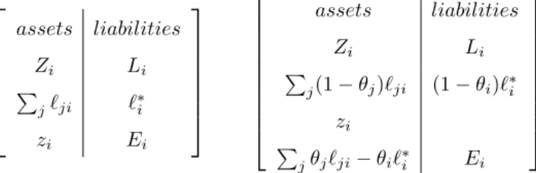
the unpaid obligations are not written off. The balance sheets before and after the clearing are given
assets liabilities Zi Li ∑ jℓji ℓ∗i zi Ei assets liabilities Zi Li ∑ j(1− θj)ℓji (1− θi)ℓ∗i zi ∑ jθjℓji− θiℓ∗i Ei Figure 1: i's balance sheet before and after the clearing
in Figure 1. Initially, i's initial total asset is Ai = Zi+
∑
jℓji+ ziand i's equity (total net worth),
Ei = Ai − (Li + ℓ∗i), is positive. The clearing has two effects on i's asset: First, the value of
i's interbank claims becomes equal to the non-reimbursed amounts (since they are not written off), second, the cash is modified by the payments made to i diminished of those made by i. The net
effect of the claims reimbursed to i is null so that i's total asset becomes equal to Ai− θiℓ∗i. The
liabilities, Li + ℓ∗i, are diminished by i's reimbursements and become equal to Li + (1− θi)ℓ∗i.
Equity is unchanged, still equal to positive Ei, due to the fact that the non-reimbursed debts are not
written off.
Default, though temporary, has nevertheless an impact if the loans to the economy are decreas-ing in the non-reimbursed claims. This arises for example if banks adjust their activity by targetdecreas-ing
a fixed leverage ratio16 λ, with λ > 1. Such a behavior may be induced by a regulatory upper-bound leverage ratio, when banks always choose the maximal activity compatible with that upper-bound.
According to the target rule, i offers new loans di defined by Ai− θiℓ∗i + di = λEi (i's equity
is not affected by di). Thus there is a substitution between i's loans to the economy and its
non-reimbursed debt. Aggregating over all banks, the substitution between the loans to the economy and the non-reimbursed interbank claims justifies to intervene so as to improve aggregate repayments.
15
Starting from Diamond and Dybvig (1983), the distinction between liquidity and solvency has been much studied in the banking literature, see e.g., Acharya et al. (2011). Even if banks' solvency is common knowledge, runs can arise as a rational phenomena. Here runs are excluded by the clearing mechanism, because it picks the maximal repayments across institutions (under equal priority) while avoiding costly premature liquidation.
16
If the cash is reimbursed at the next period, the injection is temporary, akin to lending.
The second setting is a production economy with a network of firms. The objective is justified by credit constraints as previously and the effect of time on production, drawing on Kiyotaki and
Moore (1997). At a previous date 0, firm i ordered forward some units to j to be delivered at date 1 against ℓij dollars. The gross return to production is ρ: if at date 1 i buys the units he ordered to
each supplier, the value of i's production at a future date will be ρ times the total cost, i.e., ρℓ∗i. At date 1, firms have available cash, zifor i, and receive payments for the units they deliver. They are
credit-constrained, unable to raise finance from outside investors. If i defaults against his suppliers, then he does so on a pro-rata basis and scales down his orders to θiℓij for each j, triggering possible
downsize for them. The clearing mechanism thus specifies the maximal scales of production, given the available resources and the credit constraints. The value of total production will be ρ∑iθiℓ∗i,
i.e., proportional to the realized orders' total. To improve production, one can consider for example a decrease in the price of the inputs paid at date 1 by defaulting i; such a decrease is similar to a
writing-off of part of i's debt as described in Section 3.3 and can be analyzed similarly.
3.1 Cash injection policies
Consider a regulator who is endowed with an amount of cash, denoted by m, to be injected into the institutions during a default episode. The regulator's objective is to maximize aggregate payments.
A feasible injection policy is described by a non-negative n-vector x = (xi) whose total
∑
ixiis
less than or equal to m (budget equation). xirepresents the amount received by i, which changes
ziinto zi+ xi. As a result, aggregate payments are changed from V (z) to V (z + x).
An injection policy x is said to be optimal if it maximizes V (z + x) over the set of feasible
strategies. i is said to be a 'target' if it receives a positive amount, xi > 0. The optimal injection
policies are characterized by the threat indices when m is small enough, using Proposition 1.
Proposition 2 A marginal injection of cash is optimal if it targets the institutions with the largest
threat index. The same strategy is optimal for a larger amount provided it is moderate enough to keep the defaulting set unchanged. The increase in V is equal to µmaxm where µmaxdenotes the maximal threat index.
The policy is especially simple when the injected amount is moderate since there is no need to
modify the targets. These targets may not be the institutions with the largest default ratios, since ratios and threat indices can be in different order. The targets may not be the institutions with a large
'size' either (the size can be measured in different ways, for instance by the liabilities total or the ratio of this total to the cash-flow). As clear from the expression (4), the threat index of defaulting
i is determined by its liabilities' shares (not by their levels) towards its defaulting creditors. Hence the defaulting institutions with the largest index are not necessarily those with the largest size.17 To understand better the determinants of the threat indices of defaulting institutions, let us write the
relationships (4) in matrix form18
(I − π)D×DµD = 11D. (6)
whereI denotes the identity matrix. As shown in Lemma 1 in Section 7, the matrix (I − π)D×Dis
invertible19with an inverse expressed as an infinite sum: (I−π)−1D×D =ID×D+πD×D+π(2)D×D+
... + π(p)D×D+ ... where π(p)denotes the product of π by itself p times. We thus obtain from (6) µD = 11D+ πD×D11D+ πD(2)×D11D+ ... + π(p)D×D11D+ ... (7)
which also writes for each i in D as
µi− 1 = ∑ j∈D πij + ∑ j∈D,k∈D πijπjk +· · · + ∑ jk∈D,k=1···p πij1πj1j2πj2j3..πjp−1jp+· · · (8)
Recall that µi− 1 measures the spill-over effects generated by a unit of cash injected in
default-ing i, provided there is no change in status (this is possible by scaldefault-ing the unit since no institution is at the boundary). These effects are decomposed into a sequence of reimbursements that
corre-spond to the terms on the right hand side of (8). Since defaulting i must use the received unit to reimburse its creditors, each i's creditor j receives the share πij of this unit, entirely used for
re-imbursement by those in default. This generates a first additional payment equal to i's cumulated liabilities share toward D,∑j∈Dπij, the first term on the right hand side of (8). By the same
argu-ment, each of the πij units received by defaulting i's creditor j generates
∑
k∈Dπjk extra units of
payments. Summing over all defaulting creditors of i, the second additional reimbursement equals ∑
j∈Dπij(
∑
k∈Dπjk), or
∑
k∈D(∑j∈Dπijπjk). Iterating, the additional indirect impact along a
17
This property is true at the liquidation stage given the realized default set. One may suspect that a large institution, more precisely one with large liabilities, induces important losses and defaults among its creditors when it defaults. If true, its index is likely to be large when its default. This issue is addressed in Section 4 and the illustration of Section 5.
18
There is a slight abuse of notation if some institutions are not indebted since then the matrix π is not defined on
N× N; it suffices then to consider the relative liabilities shares within indebted institutions. 19For a complete liability structure (ℓ
ij > 0 for each distinct i and j) the property follows from well known results on diagonally dominant matrices since then the total of each row of πD×Dis strictly smaller than 1 (D is a strict subset of N ). For an incomplete liability structure, the proof relies on the fact that any subset of D has necessarily creditors outside the subset: Since the zis are positive and the net worth of each defaulting institution is null, some payments must go out from the subset. This implies that, for some integer p, the total of each row of π(p)D×Dis strictly less than 1, hence the dominant eigenvalue of πD×Dis smaller than 1. Without an outside creditor for each subset, invertibility may fail,
path of p institutions, each one defaulting and indebted to its successor, is given by the p-th term in (8). This process explains why the indices are determined by the liability shares (not the absolute liabilities) within the set D and furthermore do not depend upon cash-flows' levels: The priority
of creditors triggers automatic payments that are entirely determined by the liability shares of the recipient defaulting institutions.20
The cumulated liability shares to D, the first term in (8), are a primary determinant of the indices but they are not the only ones. The 'long-run' effects of injection are measured by the additional
terms in (8) for p large, as made precise in Lemma 3 in Section 7. These terms converge to a dominant eigenvector v of πD×D, with a null vi if i is not involved in cycles. The dominant
eigenvalue ρDmeasures the persistence of the flow of repayments in D. The larger ρDis, the more
important the long-run effects are, i.e., the closer the threat index to a dominant eigenvector. This
is illustrated in the following example, where the order of the cumulated shares and indices differ.
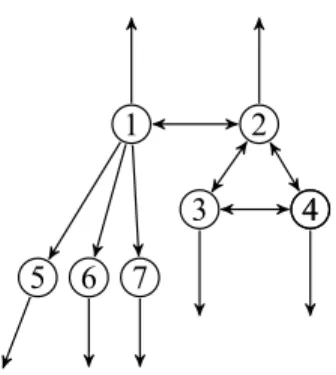
Example 2 There are 7 defaulting institutions, 1 to 7. Figure 2 represents the liabilities of D =
{1, .., 7}, in which an arrow from i to j represents a liability from i to j. Each i in D has thus a creditor outside D. The liabilities of an institution are all equal so that the shares within D are:
π1i = 1/5 for i = 2, 5, 6, 7, π2i = 1/4 for i = 1, 3, 4, π3i = 1/3 for i = 2, 4, π4i = 1/3 for
i = 2, 3 and all others are null. Consider the indices in D. Since 5, 6 and 7 are not indebted to defaulting institutions, their indices are equal to 1. The other indices are approximately µ1 =
2.2, µ2 = 3.09, µ3 = µ4 = 3.03; observe that they are not ordered as the cumulated shares to
D:1 has the largest share, 4/5, but the smallest index. This is explained by the role of the the indirect liabilities in the process following an injection of one unit into an institution. Though
1 transfers the largest amount to the defaulting institutions, 4/5, only 3/5 is transferred to 5,6,7, which transfer the received amount entirely outside D. Thus, after two 'rounds', only the liabilities
between 1, 2, 3, 4 matter with a network depicted on the right of Figure 2. This is reflected by the fact that dominant eigenvectors of πD×D, proportional to (0.1672, 0.5298, 0.5879, 0.5879, 0, 0, 0),
have null components for i = 5, 6, 7. Furthermore, others are in a different order than the shares to D. The value ρDis equal to 0.634.
The process following cash injection can be used to understand the case where some institutions are at the boundary. When an institution, say i, is at the boundary, an increase in i's cash flow has to
20An alternative interpretation of expression (6) is in stochastic term. Using that π is a transition matrix since the sum
∑
jπijis equal to 1, interpret πijas the probability of reaching j from i. Start with i in D and stop the process as soon as a safe institution is reached. Since ρD < 1, the process stops for sure. In that interpretation, the element i, j of the matrix π(p)D×Dis the probability of reaching j from i in p steps while staying all along in D and µiis the average number of times where the process stays in D when it starts at i. Probability techniques can thus be useful.
1 5 6 7 2 3 44 1 2 3 44
Figure 2: Index versus cumulated shares
be distinguished from that of a decrease: An increase has no impact on payments because i already repays its debt: ∂V
∂z+i = 0, whereas a decrease triggers i's default; thus the left derivative ∂V ∂z−i is at
least equal to 1. (Using the same argument as above, it can be computed by taking for D the set of institutions that are defaulting or at the boundary.) This explains why the value function V is not
differentiable.21
Relationships with centrality indices Threat indices have a flavor of the Katz-Bonacich (KB)
centrality indices. Given a network with incidence matrix g, the vector of KB indices is defined as (I − ag)−1g11 where a is an `attenuation' parameter, which captures the importance of indirect links. In the next example, threat indices coincide, up to a linear transformation, with KB indices on the sub-network linking defaulting institutions. Despite this similarity, our approach differs in
an important way: The threat index is based on an objective. This explains why both the subset of relevant nodes and the attenuation parameter are endogenous, respectively determined by the
subset of defaulting institutions and the number of creditors per institution.
Example 3 Let each positive liability have an identical level and each institution have the same
number of creditors, say p, hence the same total liabilities. The matrix π is thus proportional to the incidence matrix of the liabilities network: π = 1pg where gij = 1 has 1 if ℓij is positive
and 0 otherwise. Given defaulting set D, µD is equal to (
(I −1 pg)D×D
)−1
11D, which is a linear
transformation22of the KB index associated to the network gD×Dand attenuation parameter 1/p. Therefore, the more numerous creditors each institution has, the smaller the attenuation factor and the more dissipated the impact of default is along a chain of creditors.
Threat indices and the order of default in EN algorithm Let us compare the order given by
21
By the same argument, V is not differentiable with respect to the cash-flow of a defaulting j if there is a chain of defaulting creditors from j to a boundary institution.
22
1
1 2
1 3
Figure 3: Index versus order of default in EN algorithm
the threat indices with the order suggested by EN using an algorithm to compute the ratios. The
algorithm starts by setting all ratios equal to 1 and computes net-worth levels. If all net-worths are non-negative, 11 is the clearing ratio. Otherwise, ei(11) < 0 for at least one i. In that case, the
algorithm adjusts sequentially the ratios downward. Several adjustments may be necessary for a
given institution when there are cycles, contrary to the case of a chain. EN suggest that the first step at which an institution fails in the algorithm indicates its fragility. These levels are not necessarily
in the same order as the threat indices, as illustrated by the following example.
Example 4 There are three defaulting institutions, 1, 2, 3, with liabilities of equal size represented
in Figure 3. Assume that 1 is the only one to initiate default (this is possible for some values of the cash-flows). In EN algorithm, 1 defaults first, 2 second and 3 third. Since 3 is indebted outside the
defaulting set, µ3 = 1. Thus µ2 = 2 and µ1 = 4/3 (because 2/3 of it liabilities are toward
non-defaulting institutions) and it is more beneficial to inject a moderate amount of cash into 2 rather
than 1. This is due to the fact that 2/3 of the cash injected in 1 ends up outside the defaulting set.
3.2 The value of information
The optimal injection strategy uses information on the liabilities structure. In the absence of such
information, a natural strategy is a uniform strategy, which injects the same amount in each default-ing institution: xi = m/d for i in D where d is the number of elements in D and 0 otherwise. As
shown at the end of this section, a uniform strategy is indeed optimal when there is a lack of data on bilateral exposures. When there is complete information and the optimal policy can be
imple-mented, the value of information can be defined as the improvement in the aggregate repayments over the uniform policy. This value is computed in the following proposition.
Proposition 3 Let the injected amount m be allocated uniformly to the d defaulting institutions. If
D does not change, the increase in V is equal to (1d∑i∈Dµi)m. Thus, the loss with respect to the
optimal strategy is proportional to the difference (µmax−d1∑i∈Dµi).
The proof follows straightforwardly from Proposition 1 using thatthe marginal increase in V due
to the difference between the maximal index and the average index over the defaulting set. In Example 2, the maximal index is equal to 3.09 and the average one to 2.05, so that the value is quite large, roughly equal to m.
When the cumulative liability shares differ, the indices differ as well23 and the value of in-formation is positive. Note that the indices may be in a different order than the cumulated shares
because of chain effects (see e.g. Example 4) so that the information on the cumulated shares is not enough to implement the optimal policy. When the cumulative liability shares within D are equal,
the value of information is null was shown in the next example.
Example 5 Let the cumulative liability shares within D be equal: The sum∑j∈Dπij is equal to
σDfor each i in D. In that case, the indices in D are all equal: µi = 1−σ1
D for i in D. The value of
information is null and any moderate injection into D is optimal. The injection benefit itself may be
large if σDis close to 1, that is, if defaulting institutions are mainly indebted between themselves.
When there is a lack of data on bilateral exposures, the log-fitting method is used to estimate the
missing data given the available information (see for example Upper and Worms 2004 and Elsinger, Lehar, and Summer 2004). Let us consider the situation in which the total amount of liabilities and
total amount of loans are known but there is no specific information on bilateral exposures. In that case, the estimated i's liabilities shares are independent of i, equal to the overall proportions of the
loans, pj = ∑
i∈Nℓij
∑
i,k∈Nℓik for j. This implies that the cumulated shares within a default set D are
estimated all equal to σD =
∑
j∈Dpj. Hence the threat indices are equal as well (see example 5),
equal to 1−σ1
D: A uniform strategy is optimal and the information on bilateral liabilities is null.
Therefore, the log-fitting model surely underestimates the value of information.24
3.3 Alternative policies: Transfers across institutions
This section examines alternative policies based on transfers within institutions, without external intervention. A first policy is similar to the injection policy considered previously but the cash is
injected by the safe institutions instead of a regulator. An alternative policy asks the creditors to an institution in difficulty to write-off part of their claims on that institution. A writing-off of part of
the claim from safe j to defaulting i amounts to a decrease in ℓij.
For each policy, the precise contribution on each safe institution does not matter as long as
the safe institutions remain safe: For the injection policy, only the total injected amount matters.
23
The indices are equal when µDis equal to µ max
11D. From (6), this is equivalent to µmax(I − π)D×D11D = 11D, which writes as (µmax− 1)11D= µmaxπD×D11D; hence the cumulated shares within D are equal.
24
It also underestimates the benefit of an injection if µmax, the maximal index of the 'true' matrix, is larger than1−σ1
D,
For the writing-off policy, the impact on the repayments of a writing-off of part of i's liabilities only depends on the total reduction in i's debt, not on the precise amount written off by each safe creditor. As a result, the optimal policies described in the following proposition do not specify the
contributions. (Of course, these contributions could be made precise ex ante, so as to satisfy some fairness or participation constraints.)
Proposition 4 A transfer of one unit from the safe institutions to the defaulting ones is optimal if it
targets those with the largest index.
A marginal writing-off by safe institutions of one unit of their claims on defaulting i leads to increase V by θi(µi − 1). It is thus optimal first to write-off part of the claims of the institutions
with the largest θi(µi− 1).
According to the proposition, writing-off part of the claims of the safe creditors of a defaulting
institution i results in an increase in the overall payments if i is also indebted to another defaulting institution (µi > 1), and leaves them unchanged otherwise. That repayments never decrease is not
obvious because i reimburses less to safe institutions due to the writing-off of their claims. How-ever, i's total reimbursements are unchanged since i defaults; thus a larger proportion is allocated
towards defaulting creditors, which triggers further repayments. The larger µi, the more
benefi-cial the impact on subsequent creditors, as in the case of a cash injection; the larger θi, the more
important the amount redistributed towards defaulting institutions.
4
Ex ante value of raising capital
So far, the analysis has taken place at the liquidation of the liabilities. This section evaluates the impact of an increase in the requirement on capital at an ex ante stage. Specifically, it considers
the situation in which the increase in capital has to be invested in a risk-free asset, keeping risky investments and liabilities unchanged.
Initially, institutions expect possibly random cash-flows from their investments,ezifor i, where
eindicates the random variable before its realization. Let V be the payment value associated to the cross-liabilities. The aggregate repayments will be V (z) if the realized value for the cash-flows is z, hence the expected repayments are equal to E[V (ez)]. Consider an increase in capital, kifor
i, invested in a risk-free asset with null net return (to simplify notation); i's cash-flow is changed into ezi+ ki and the expected repayments into E[V (ez + k)]. It follows that raising i's capital by
1 (marginal) unit raises expected repayment by E[µi(ez)]. This defines the marginal value of i's
denotes the set of defaulting institutions given z. P denotes the probability distribution of ez and P[i ∈ D(z)] the probability of the set {z s.t. i ∈ D(z)}.
Proposition 5 The marginal value of i's capital, vi = E[µi(ez)], is equal to P[i ∈ D(z)](1 + αi),
where αiequals the expectation of the spill-over effects conditional on i defaulting:
αi = ∑ j πijP[j ∈ D(z)|i ∈ D(z)] + ∑ j,k πijπjkP[j and k ∈ D(z)|i ∈ D(z)] + + ∑ j,k,l πijπjkπklP[j, k and l ∈ D(z)|i ∈ D(z)]...
The marginal value of i's capital is thus (not surprisingly) increasing in its probability of default.25It
is also increasing in the expectation of the spill-over effects conditional on i defaulting, αi, hence in
the weakness and default of i's creditors, direct or indirect, when i is defaulting. The spill-over term
is thus increasing in the correlation in defaults between i and its creditors. A positive correlation in defaults is induced by a positive correlation in the cash-flows, as results from similar investment
portfolios, as studied in papers referred in the introduction. It is also induced by the cross-liabilities themselves, even if the cash-flows are independent, as shown in the next corollary.
Corollary 1 Letbπij = πijP[i ∈ D(z)] for each i and j, and26 bµ = (I − bπ)−111.
If the defaults are independent, then vi=P[i ∈ D(z)]bµi.
If the cash-flows ˜zi are independent, then the defaults are positively correlated, i.e., for each
subset S of N P[S ⊂ D(z)] ≥ Πi∈SP(i ∈ D(z)), and vi≥ P[j ∈ D(z)]bµi for each i.
bµ is a threat index computed as if the default set is the whole set N and each share πijis multiplied
by the creditor's default probabilityP[j ∈ D(z)]. Under independent defaults, the marginal value of i's capital is equal to its probability of default multiplied by bµi.27 Though, defaults are not
independent but positively correlated when cash-flows are independent, due to the liabilities which
'propagate' default. The effect is to increase the marginal value.
Impact of the size There is a debate about the impact of the size of the institutions on systemic risk
(for a recent analysis and the references therein, see De Jonghe, Diepstraten, Schepens 2015). To investigate this issue, I compute here the marginal values of capital for institutions that differ only in their size, meaning that they are 'proportional': the distribution of their cash-flows are equal up
25
Note that an institution that never initiates default may nevertheless defaults due to default on its loans. This is reminiscent of the distinction put forward by Tarashev, Borio, and Tsatsaronis (2010) as the 'participation' to default.
26
The matrixπ is positive with a dominant eigenvalue strictly smaller than 1 since the probabilities of default are notb
all equal to 1. ThusI − bπ is invertible with a positive inverse.
to a scale factor and their liabilities and loans are proportional with the same scale factor. Formally institution 1 is proportional to institution 2 with scale factor λ if the distribution of 1's cash-flowez1
is the same as that of λez2, and 1's liabilities and loans toward institutions other than 2 are λ times
those of 2, and 1's liability toward 2 is λ times 2's liability toward 1. Thus 1's and 2's liabilities' shares towards other institutions are equal, π1,i = π2,ifor i > 2 and π1,2 = π2,1.
Furthermore, to isolate the size effect, let us assume that 1 and 2 cash-flows are 'conditionally proportional ', i.e., that a low realization of 1's cash-flow relative to 2 's (or the reverse) is
inde-pendent of others' cash flows. Formally, given (z1, z2), denote (zσ1, zσ2) = (λz2, z1/λ): 1 and 2
cash-flows are exchanged and adjusted to the size. Thus,ez1σ is distributed as λez2, hence asez1 by
assumption; similarlyezσ2 andez2are identically distributed. The cash-flows of institutions 1 and 2
are said to be conditionally proportional if the distributions of (ez1,ez2) and (ezσ1,ez2σ) conditionally
on z−12are identical. Of course, 1 and 2 cash-flows are conditionally proportional if all cash flows are independent.
Proposition 6 Let institutions 1 and 2 differ in size, with 1's size λ times 2's size for λ > 1. Assume
their cash-flows to be conditionally proportional. Then
E[µ1(ez)|z1 ≤ λz2]≥ E[µ2(ez)|z1 ≥ λz2] and E[µ2(ez)|z1≤ λz2]≥ E[µ1(ez)|z1 ≥ λz2]. (9)
The marginal value of capital is equal to the mean of the two conditional expected values (vi = 1
2(E[µi(ez)|z1 ≤ λz2] + E[µi(ez)|z1 ≥ λz2]) for each i) so the values differ but cannot a priori
ordered. The reason is that the default set depend on whether (z1, z2) or (z1σ, z2σ) is realized. Thus,
though the distributions of (z1, z2) and (zσ1, z2σ) are identical conditional on others' cash flows, the
expected threat indices depend on which institution is relatively weaker. Specifically, the larger institution has a larger impact on default and this works in two directions. The impact is harmful
when 1 is relatively weaker than 2: For (z1, z2) with z1 ≤ λz2, the default set can only be larger
than in the symmetric situation (zσ1, zσ2) where 2 is weaker than 1 (see the proof): This explains the left-hand-side inequality of (9). Conversely, the impact of the size is beneficial when 1 is relatively
stronger than 2: For (z1, z2) with z1 ≥ λz2the default set can only be smaller than in the symmetric
situation (zσ
1, z2σ): This gives the right-hand-side inequality of (9). Though the marginal values of
capital cannot be compared, that of institution 1 is larger if 1 and 2 have few chances to default together: In that case, 1 defaults only if z1 < λz2and 2 only if z1 > λz2. The marginal values are
thus equal to half the expressions on the left-hand side inequality of (9). In that case, the institution with the larger size should have a relatively larger capital.
5
European cross-liabilities
This section illustrates the method on the consolidated foreign claims for 10 EU countries: Austria, Belgium, France, Germany, Greece, Ireland, Italy, the Netherlands, Portugal, Spain. These claims
are those of reporting banks in one country on debt obligations of another country. The data is available from the Bank of International Settlements. The exercise can be viewed as a thought
experiment in which all these claims are liquidated. How much will a country reimburse assuming that each country allocates a fraction of its GDP to the liquidation of its foreign claims? (Since
the claims are consolidated, the default of a country, in particular the default on its governmental bonds, is internalized among its residents. This suppresses the corresponding spill-over effects.)
Liquidation is based on a fraction of the GDPs at the time of liquidation. Specifically, given the level of GDPiin country i at the year of reference, i's 'cash-flow' available allocated to liquidation
is given by
ezi = ekiGDPi
Ex ante, the factor ki is perceived as random, reflecting the uncertainty on growth rate and the
future GDP level or on political factors such as the resistance to reimburse within the country. In the reported simulations, the reference year is 2008 and the simplest assumptions on eki are taken:
they are log-normally and independently distributed, with the same mean m and standard error v with m = 1/2 and v = 1/8. Simulations with 1000 draws are run for three years, 2009, 2010 and
2011. To concentrate on the impact of cross-liabilities only, the same reference year is used for the three years so thatezifollows the same distribution: The changes linked to default are only due to
changes in the cross-liabilities.
Let us first consider the situation in which all the zis are equal to their expected value, here
half of GDPi. Belgium and Ireland initiate default, since their 'net-worths' are negative as can be
seen from Table 1. Their default does not propagate, i.e., no other country defaults at the clearing
ratios, so Table 2 only reports the ratios and threat indices for Belgium and Ireland. Their indices only depend on the liabilities' shares between them. Belgium's index is much smaller than Ireland's
one due to the asymmetry in their liabilities: Belgium's liabilities share to Ireland is much smaller than that of Ireland to Belgium. More generally, liabilities are very asymmetric, and this plays an
Table 1: Net-worths at the mean values. Unit: 100 millions of dollars
Aust Belg F rance Germany Greece Ireland Italy N etherlands P ort Spain
2009 335 −905 23278 18028 153 −1346 6001 5727 142 3424 2010 543 −43 19257 16733 668 −417 7776 4956 526 4838 2011 598 −318 18043 16764 866 −1150 8751 4847 594 5842
Table 2: The clearing ratio and threat index at the mean values for Belgium and Ireland
Belg Ireland Belg Ireland
θ θ µ µ 2009 0.776 0.664 1.014 1.162 2010 0.97 0.845 1.015 1.171 2011 0.868 0.494 1.001 1.155
Let us consider now the effect of the shocks on ki. A country initiates default when its
cash-flow, kiGDPi, is smaller than its net liabilities (the difference between total liabilities and loans)
ℓ∗i−∑jℓji, or equivalently when ki< ρiwhere ρiis equal to the ratio of i's net liabilities to GDP.
The ρis are reported in Table 3.
Table 3: Net liabilities to GDP ratio ρi
Aust Belg F ra Germ Greece Ireland Italy N eth P ort Spain
2009 0.3989 0.7282 −0.5623 −0.0915 0.4541 1.2104 0.1995 −0.3114 0.4465 0.2733 2010 0.3363 0.5110 −0.3788 −0.0490 0.2991 0.7200 0.1106 −0.2022 0.3015 0.1797 2011 0.3198 0.5803 −0.3234 −0.0500 0.2397 1.1071 0.0617 −0.1867 0.2757 0.1132 A country with a negative ratio never initiates default. This is the case for France, Germany, and the Netherlands. We will see that they never default through contagion as well. A country with a
positive ratio initiates default with the probability that the lognormal distribution with mean 1/2 and standard error 1/8 is less than ρi. They are reported in Table 4. The decrease in the probabilities
in 2010 is due to the general decrease in the net liabilities and the ρis for the vulnerable countries
between 2009 and 2010.
Table 4: Probability to initiate default
Aust Belg Greece Ireland Italy P ort Spain
2009 0.4856 0.8183 0.5663 0.9561 0.1303 0.5559 0.2643 2010 0.3805 0.6378 0.3126 0.8135 0.0201 0.3170 0.0988 2011 0.3507 0.7096 0.2016 0.9414 0.0015 0.2688 0.0220
Table 5 gives the expectation of the clearing ratios, unconditional and conditional on the default of the country, threat indices, the spill-over index αi defined in Proposition 5 and the number of