Investigating the Role of Real Divisia Money in Persistence-Robust Econometric Models

(1)

HAL Id: hal-00984827

https://hal-paris1.archives-ouvertes.fr/hal-00984827

Preprint submitted on 28 Apr 2014

HAL is a multi-disciplinary open access

archive for the deposit and dissemination of

sci-entific research documents, whether they are

pub-lished or not. The documents may come from

teaching and research institutions in France or

L’archive ouverte pluridisciplinaire HAL, est

destinée au dépôt et à la diffusion de documents

scientifiques de niveau recherche, publiés ou non,

émanant des établissements d’enseignement et de

recherche français ou étrangers, des laboratoires

Investigating the Role of Real Divisia Money in

Persistence-Robust Econometric Models

Ryan S. Mattson, Philippe de Peretti

To cite this version:

Ryan S. Mattson, Philippe de Peretti. Investigating the Role of Real Divisia Money in

Persistence-Robust Econometric Models. 2014. �hal-00984827�

(2)

Investigating the Role of Real Divisia Money in

Persistence-Robust Econometric Models

Ryan S. Mattson

1

_{Philippe de Peretti}

23

March 4, 2014

1_{Department of Economics, Rhodes College, 320 Buckman Hall 2000 N Parkway, Memphis, TN. tel.}

901-843-3122, mail mattsonr@rhodes.edu

2_{Contact Author. Centre d’Economie de la Sorbonne, Université Paris1 Panthéon-Sorbonne, Maison}

des Sciences Economiques, 106-112 Boulverd de l’Hôpital, 75013 paris, France. tel. 0033144078746, mail philippe.de-peretti@univ-paris1.fr

3_{This project has received funding from the European Union’s Seventh Framework Programme}

(FP7-SSH/2007-2013) for research, technological development and demonstration under grant agreement no grant agreement 320270 - SYRTO

(3)

Abstract

This paper investigates the causal relationships between real money and real activity. Whereas previous literature has mainly focused on simple-sum aggregates, we instead use Divisia ones, thus avoiding the so-called Barnett Critique. Standard Granger non-causality tests are implemented in two di¤erent frameworks: Fully Modi…ed VAR’s (Phillips, 1995) and surplus-lag VARX models (Bauer and Maynard, 2012). These two environments allow modeling mixtures of I(0)/I(1) variables with possible cointegration without pretesting for integration nor for the dimension of the cointegration space. Moreover the latter method is also robust to various other forms of persistence such as local-to-unity processes, long memory/fractional integration, or unmodeled breaks-in-mean in the causal variables. By implementing the tests on di¤erent sub-samples identi…ed by standard structural break tests, and using three di¤erent measures of money (DM4, DM4- and DM3), the tests suggest a unidirectional causality from activity to money. Moreover, from one period to another, the whole causal structure of the systems seem to change, as well as the stationarity of the series. At last, the two methodologies return similar results.

(4)

1 Introduction

Economists have long been interested in the role of money in the economy, especially regarding its role as a leading indicator for future activity. Following the early works of Sims (1972, 1980), most researchers have focused on non-causality tests à la Granger (1969) in Vector Auto-Regressions (VAR). Among many others, Hayo (1999) and Walsh (2003) survey this vast literature, both emphasizing the contradictory results found by many researchers, showing that it is not possible to draw clear conclusions about the role of money in the economy. A similar conclusion was previously reached by Stock and Watson (1989), noticing that “Researchers using only slightly di¤erent speci…cations have reached disconcertingly di¤erent conclusions”.

In this paper, we argue that such instability of results may have at least two distinct sources: i) Measurement errors in monetary aggregates due to inappropriate aggregation methods and, ii) Two-stage inference in econometric models.

Concerning the former point, as suggested in a number of seminal publications (Barnett, 1980; Barnett, O¤enbacher and Spindt, 1981, 1984; Barnett and Serletis, 2000), there exists an internal inconsistency between the microeconomics used to model the private sector, and the aggregator functions used to compute monetary aggregates by central banks. As a corollary, simple-sum ag-gregates, computed by central banks, are likely to return ‡awed measures of money, being based on the unrealistic assumption of perfect substitutability of assets. This critique, known as the Barnett Critique, de…ned by Chrystal and MacDonald (1994), strongly a¤ects the results given by macroeconomic models, implying that outcomes of studies using simple-sum aggregates are mis-leading. Belongia (1996) has investigated the empirical validity of this Critique by reexamining several studies on money, replacing the ‡awed simple-sum measures with theoretically-consistent ones. He shows that the original conclusions are then deeply altered. Theoretically-consistent measures of money have been used in a number of studies such as Barnett, Fisher and Serletis (1992), Chrystal and MacDonald (1994) who study the relationship between money and GDP, Schunk (2001) focusing on the predictive content of money, Serletis (1991) and Serletis and King (1993) or Yue and Fluri (1991). Other recent works also include Darrata et al. (2005), Bar-nett, Chauvet and Tierney (2009), Belongia and Ireland (2012a, 2012b) or Rahman and Serletis (2012).

Concerning the latter point, classical tests of non-causality rely on pre-tests (…rst-stage in-ference) on the persistence of the series. For instance, if all series are stationary, a simple VAR in levels is estimated, whereas if the series are integrated but not cointegrated, a VAR in …rst

(5)

di¤erences is used. If additionally, cointegration is present, then a Vector Error Correcting Model (VECM) is estimated (Toda and Phillips 1993, 1994). This simple example emphasizes a general method consisting of: i) Trying to identify the correct underlying Data Generating Process (DGP) according to pre-tests for stationarity/cointegration (…rst-stage inference), and ii) Testing for non-causality in the estimated DGP (second-stage inference). Nevertheless, in empirical work, due to lack of power of stationarity tests, estimating the “true” DGP may be di¢cult, as well as di¤erentiating between the di¤erent kind of persistence as local-to unity processes, (Phillips, 1987; Chan, 1988), or long memory/fractional integration; a problem that deeply worsens if structural breaks are present (Diebold and Inoue, 2001). Hence, inappropriate persistence modelling, and thus inaccurate DGP identi…cation may lead to incorrect inference and cascading errors in non-causality tests.

The goal of the paper is to study the causal relationships between real money and activity by taking into account the two above points. To avoid the Barnett Critique, we use theoretically-consistent measures of money, i.e. Divisia indices. Concerning the econometric models, we follow Bauer and Maynard (2012), suggesting agnostic approaches to the form of persistence, that is suggesting tests that are robust to the various forms of persistence, without any pre-testing. In causality testing, to our knowledge, two approaches can be used, i) The Fully-Modi…ed VAR (FM-VAR) of Phillips (1995), extending the Fully Modi…ed ordinary least square of Phillips and Hansen (1990), ii) The surplus-lag VARX model of Bauer and Maynard (2012), based on Toda and Yamamoto (1995), Dolado and Lütkepohl (1996) or Saikkonen and Lütkepohl (1996). Whereas the FM-VAR is designed to model a mixture of I(0)/I(1) variables with possible but unde…ned cointegration, the Bauer and Maynard (2012) surplus-lag VARX approach possesses basically the same features, but goes further. Indeed, the causality test remains robust, when the causal variable has long memory/fractional integration, can be modeled as a local-to-unity process, or contains a certain amount of unmodeled breaks in mean. In this latter case, the noncausality test is interpreted as a co-breaking test.

The main results of the paper are twofold: i) Using three di¤erent Divisia monetary aggre-gates, tests support an unilateral causality from real activity to real money, ii) Over the di¤erent sub-periods, the whole causal structure of the systems, as well as the long term relationships seem to change.

This paper is organized as follows. Section two focuses on monetary aggregation and presents the theoretically consistent Divisia aggregates. Section three introduces the econometric method-ologies. In Section 4, we …rst test for structural breaks on the growth rates of the series, and

(6)

then implement non-causality tests on di¤erent sub-periods. At last Section 5 concludes and discusses the results.

2 The theoretical approach to monetary aggregation

In this section, we brie‡y recall the theoretical approach to monetary aggregation. Let xt =

(x1t; :::; xkt)0 and mt= (m1t; :::; mpt)0 be respectively two vectors of real consumption goods and

real monetary assets in period t; t = 1; :::; T: Let ltbe leisure. Assume that data are rationalized

by a well-behaved utility function:

Ut= U (xt; mt; lt) (1)

i.e. each bundle (x1t; :::; xkt; m1t; :::; mpt; lt)0is the solution of the utility maximization program1,

where the nominal price of money, for an asset mitis de…ned according to Barnett (1978):

pnit= pt Rt rit 1 + Rt ; i = 1; :::; k (2) Where: Rt is a benchmark rate,

ritis the asset’s own rate,

pt is a consumer price index.

To allow for aggregation, further assume that the utility function (1) is weakly separable over the monetary assets, and thus admits a rewriting:

Ut= U (xt; mt; lt) = V (xt; U1(mt); lt) (3)

Where:

V (:) is a strictly increasing function, known as the macro-function,

U1(:) is the monetary sub-utility function, known as the micro-function, which, if homothetic, is

also the aggregator function.

The above weakly separable utility structure ensures that an aggregate exists over money2. Following Diewert (1976, 1978), if the preferences over the monetary assets are homothetic, then

1_{For theoretical justi…cations of money in the utility function, see Feenstra (1986) and Poterba and Rotemberg}

(1987).

2_{Notice that here weak separability is assumed but not tested. For more formal testing procedures, see for}

example Varian (1983), Swo¤ord and Withney (1987, 1988), de Peretti (2007), Barnett and de Peretti (2009), or Fleissig and Whitney (2003, 2005).

(7)

U1(:) is interpreted as the aggregator function. An index number Q(mt+1; mt; pnt+1; pnt), must therefore satisfy: Q(mt+1; mt; pnt+1; pnt) = U1(mt+1) U1(mt) (4) If preferences are non-homothetic, the aggregator function is no longer the sub-utility function, but the distance function. The distance function D(U1; mt) = maxlfl : U (mt=l) U1g returns

by what proportion one has to in‡ate or de‡ate the vector mtin order to reach the utility level

U1. A consistent aggregate is given by:

Q(mt+1; mt; pnt+1; pnt) =

D(U1; mt+1)

D(U1; mt)

(5) Diewert (1976, 1978, 1980) proved that in both case cases Q(mt+1; mt; pnt+1; pnt) can be

nonpara-metrically and consistently estimated as: Q(mt+1; mt; pnt+1; pnt) = p Y i=1 mit+1 mit (sit+1+sit)=2 (6) Where:

sit is the budget share for the monetary asset i in period t,

U1=

p

U1(mt+1)U1(mt).

Clearly, (6) is a discrete approximation of the continuous Divisia index.

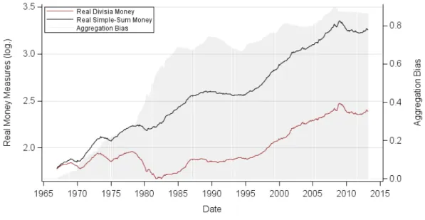
In their seminal paper, Barnett, O¤enbacher and Spindt (1984) present a very comprehensive survey of the so-called Divisia aggregation. They show that very di¤erent conclusions are drawn when one considers Divisia aggregation, rather than simple-sum aggregates, the latter being valid only if the assets are substitutes, which is an unrealistic assumption. As an illustration, Figure (1) plots two monetary aggregates: The DM4 (see below), and the simple-sum built by adding the component levels of the DM4 assets. Both aggregates are divided by a consumer price index and are in log-form. On the same …gure, we plot (right scale) the aggregation bias, which is computed as the di¤erence between the two indices. Clearly, the error is not constant over time and dramatically increases up to the early 90’s, according to the explosion of …nancial innovations. After the early 90’s, the bias decreases, and then constantly increases at a lower growth rate. Notice that the bias re‡ects di¤erent trends in the two series. The time-varying nature of the bias implies that simple-sum aggregates can not be used as proxies of Divisia aggregates.*

(8)

Figure 1: Real DM4, simple-sum over the same components as the DM4, aggregation bias. (shaded area, right sclale).

3 Non-causality tests in persistence-robust econometric

mod-els

To analyze the role of Divisia money in the economy, we use standard Granger non-causality tests in VAR models. Two frameworks are considered that do not impose pre-testing for persistence nor for cointegration: The FM-VAR approach of Phillips (1995), and the surplus-lag VARX model of Bauer and Maynard (2012). The former approach allows modeling a mixture of I(0)/I(1) variables without specifying the order of integration of each component, nor the dimension of the cointegration space. The latter framework is more general since it also takes into account other forms of persistence in the causal variable as local-to-unity processes, fractional integration/ long memory and unmodeled structural breaks-in-mean in the causal variable. We …rst describe the FM-VAR method.

3.1 The Fully-Modi…ed approach to VAR modeling

Let ytbe a k-vector time series generated by the …nite-order VAR of order p, VAR(p):

(9)

Table 1: SupFT(l + 1jl) sequential tests for structural breaks, monetary components div4rt, Lag = 2, h = 0:1 l + 1 l SupFT(l + 1jl) Cut of f (5%) 1 0 23.22 14.60 2 1 14.37 16.53 3 2 08.57 17.43 Final (global) Estimates of the Single Break: Sep1981 div4mrt, Lag = 2, h = 0:1 l + 1 l SupFT(l + 1jl) Cut of f (5%) 1 0 31.11 14.60 2 1 22.98 16.53 3 2 16.46 17.43 Final (global) Estimates of the Two Breaks: Feb1996, Mar2008 div3rt, Lag = 2, h = 0:1 l + 1 l SupFT(l + 1jl) Cut of f (5%) 1 0 44.99 14.60 2 1 19.90 16.53 3 2 15.81 17.43 Final (global) Estimates of the Two Breaks: Apr1995, Mar2008 where: J(L) = p P i=1 JiLi 1; "t Niid(0; "").

(7) can be equivalently re-written as:

yt= B(L) yt 1+ Ayt 1+ "t (8) where: B(L) = p 1_P i=1 BiLi 1with Bi= p P j=i+1 Jj, and A = J(1): or as: yt= B(L) yt 1+ yt 1+ "t (9) where: = A Ik

(10)

This latter representation is the Vector Error Correction form representation of a VAR process. The A matrix or ( ) contains all relevant information about the long-term relationships. Now, re-write model (8) as:

yt = Bzt+ Ayt 1+ "t (10) = F xt+ "t (11) Where: zt= ( y0t 1; :::; y0t p+1)0: xt= ( yt 10 ; :::; yt p+10 ; yt 10 )0; B = [B1; B2; ::; Bp 1]:

Or in matrix form as:

Y0 _{= BZ}0_{+ AY}0

1+ E0 (12)

= F X0_{+ E}0 ₍₁₃₎

Where:

F = [B1; :::; Bp 1; A]:

Since the above model can not be e¢ciently estimated by Ordinary Least Square (OLS) due to a second order (endogeneity) bias, Phillips (1995) suggest applying the Fully Modi…ed estimator (Phillips and Hansen, 1990) to the system. De…ne b"y and byy as estimates of the two-sided

long-run covariance matrices of respectively t = (b"t = yt F xt; yt 1) and yt 1; where b"t

are the OLS residuals of model (8). Also de…ne b" y and b y y as estimates of the one-sided

long-run covariances matrices of respectively t = (b"t = yt F xt; yt 1) and yt 1. Notice

that both types of matrices are kernel estimates. For instance b"y and b" yare computed as:

b"y= T_P1 j= T +1 w(j=k1)b(j) (14) b" y= T_P1 j=0 w(j=k1)b(j) (15) Where:

w(j=k1) is a kernel smoothing function, k1 is the bandwidth or truncation parameter, b(j) is the standard covariance estimator, T 1PT

t=1 t 0 t+j

The FM-VAR estimator is then de…ned as: b

F+_{= [Y}0_ZjjY0_Y

(11)

Where:

jj is the horizontal stacking operator, Y0

1= Y01 Y02:

Compared to the standard FM estimator for OLS, no correction for autocorrelation is made. Thus, the only correction is for endogeneity.

De…ning bF = [Y0_ZjjY0_Y

1](X0X) 1 as the simple OLS estimator, (16) can be re-written in

order to make apparent the correction for endogeneity: b

F+= bF [b"ybyy1( Y01Y 1 T b y y)](X0X) 1 (17)

A non-causality test from variable j in equation i, amounts to testing: B1[ij] = ::: = Bp 1[ij] = A[ij] = 0

which can be stated as:

H0: Rvec( bF+) = 0 (18)

where R is a (q 1) suitable selection matrix, with here q = p. Then the corresponding Wald test is given by:

W+ = T (Rvec( bF+))0_[R(b

" T (X0X) 1)R0] 1(Rvec( bF+)) (19)

Phillips (1995) proved that under the null, W+ _{is asymptotically bounded by a Chi-squared}

distribution with q degrees of freedom, q being the rank of R.

3.2 The surplus-lag VARX model

Alternatively, one may also consider surplus-lag models to test for non-causality between two variables, y1tthe dependent one and y2t the exogenously modeled forcing (causal) variable, given

a set zt= (y3t; ::; ykt)0 of control variables. We here follow Bauer and Maynard (2012), extending

and simplifying Toda and Yamamoto (1995). In our framework, i.e. the causality between two series, write down and estimate the single equation of interest of a surplus-lag VARX(p; p1), here

a Auto-Regressive ARX(p; p1) process:

y1t= p X j=1 1 jy1t j+ 2jzt j + p1+1_P j=1 3 jy2t j+ "t (20)

and jointly test for 31= 3

2= ::: = 3

p1= 0 using a standard Wald tests3.

(12)

The two models are clearly complimentary. On the one hand, if series are I(0)/I(1) and cointegration is present, the FM-VAR is e¢cient, unlike the VARX which forces an extra lag. Nevertheless, as shown by Bauer and Maynard (2012) based on Monte Carlo simulations, e¢-ciency losses have a very limited impact on the power of causality tests. On the other hand, for local-to-unity processes, the causality tests in FM-VAR’s may not behave well, as shown by Yamada and Toda (1997), which is a case for which the VARX is designed for. Hence, di¤erent informations between the two tests may indicate di¤erent kinds of persistence. For other kinds of persistence, such as long memory, nothing is known for the FM-VAR.

We next turn to implementations4_.

4 Implementing the tests

The role of real money balance e¤ects has recently been reconsidered by Favara and Giordani (2009), using a structural VAR, imposing restrictions consistent with the New Keynesian frame-work. They suggest that real money balances shocks may have a signi…cant e¤ect on output and prices. Dorich (2009) reaches a very similar conclusion using a money-in-the-utility model. Interestingly, he concludes that such e¤ects may be based on a non-separable utility function, a fundamentally di¤erent framework from ours. Those conclusions are in sharp contrast with Woodford (2003) and Ireland (2004), who show the negligible impact of real money. All these articles used inconsistent measures of money. Here, we reconsider their conclusions using three di¤erent theoretically-consistent measures of broad money. We …rst describe the data and ana-lyze their statistical properties in terms of structural breaks, and the implement the described non-causality tests.

4.1 Data

Let y1

t = (div4rt; indprot; irstt; irltt; 12pt)0, yt2 = (div4mrt; indprot; irstt; irltt; 12pt)0 and

yt3= (div3rt; indprot; irstt; irltt; 12pt)0be k-vectors of variables being integrated of order 1 or 0,

where: div4rt, div4mrtand div3rtare respectively the logarithms of the real Divisia DM4,

DM4-and DM3 indices; indprotis the logarithm of the Industrial Production Index, used as a proxy

of the real activity; irsttand irlttare respectively short (three-month) and long-term (one year)

interest rates and 12ptis the Consumer Price Index in‡ation rate. All data are on a monthly

basis, and span, for the United States, the period covering January 1968 to December 2012. Data

4_{All the routines, i.e the FM-VAR model, the surplus-lag VARX as well as the Bai and Perron (1998) tests}

(see below) are programmed using SAS/IML and are available under request at the corresponding author email adress: philippe.de-peretti@univ-paris1.fr

(13)

Table 2: SupFT(l + 1jl) sequential tests for structural breaks, Other components ( 12pt), Lag = 3, h = 0:1 l + 1 l SupFT(l + 1jl) Cut of f (5%) 1 0 43.40 16.76 2 1 21.92 18.56 3 2 19.40 19.53 4 3 10.75 20.24 Final (global) Estimates of the Three Breaks: Nov1982, Oct1991, Oct2007

indprot, Lag = 3, h = 0:1

l + 1 l SupFT(l + 1jl) Cut of f (5%)

1 0 34.96 16.76 2 1 09.42 18.56 3 2 07.96 19.53 Final (Global) Estimates of the Single Break: Dec1981 irstt, Lag = 1, h = 0:1 l + 1 l SupFT(l + 1jl) Cut of f (5%) 1 0 07.39 12.25 2 1 04.25 13.83 3 2 04.01 14.73 irltt, Lag = 2, h = 0:1 l + 1 l SupFT(l + 1jl) Cut of f (5%) 1 0 12.09 14.06 2 1 08.38 13.83 3 2 06.50 14.73

are collected from the Federal Reserve of St Louis5_{, except the Divisia indices computed by the}

Center for Financial Stability6 _{(CFS). The CFS monthly reports statistics for Divisia indices as}

the broad DM4, DM4-, which is DM4 without short term treasury bills, and DM3, which does not include treasuries nor commercial paper, corresponding to the discontinued M3 aggregate. Barnett et al. (2012) describe the construction of those monetary aggregates. The nominal price of money for each asset is computed using a corresponding interest rate and a benchmark rate; interest bearing checking accounts are paired with the national average interest rate on those accounts, for example. The benchmark rate is chosen as a maximum rate among the ‘basket’ of component rates along with other comparable loan rates. Included in this basket is a short

5_{http://research.stlouisfed.org/fred2/} 6_{www.centerfor…nancialstability.org}

(14)

Table 3: SupFT(l + 1jl) sequential tests for structural breaks in variances for the two interest rates irstt, Lag = 0, h = 0:1 l + 1 l SupFT(l + 1jl) Cut of f (5%) 1 0 78.12 12.25 2 1 13.25 13.83 3 2 12.66 14.73 Global Estimates of the Two Breaks: Sep1982, Nov2007 irltt, Lag = 1, h = 0:1 l + 1 l SupFT(l + 1jl) Cut of f (5%) 1 0 22.13 12.25 2 1 13.35 13.83 3 2 12.71 14.73 Global Estimates of the Two Breaks: Jul1979, Nov2007

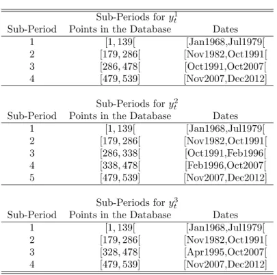
Table 4: Sub-Periods for the non-causality tests Sub-Periods for y1

t

Sub-Period Points in the Database Dates 1 [1; 139[ [Jan1968,Jul1979[ 2 [179; 286[ [Nov1982,Oct1991[ 3 [286; 478[ [Oct1991,Oct2007[ 4 [479; 539] [Nov2007,Dec2012] Sub-Periods for y2 t

Sub-Period Points in the Database Dates 1 [1; 139[ [Jan1968,Jul1979[ 2 [179; 286[ [Nov1982,Oct1991[ 3 [286; 338[ [Oct1991,Feb1996[ 4 [338; 478[ [Feb1996,Oct2007[ 5 [479; 539] [Nov2007,Dec2012] Sub-Periods for y3 t

Sub-Period Points in the Database Dates 1 [1; 139[ [Jan1968,Jul1979[ 2 [179; 286[ [Nov1982,Oct1991[ 3 [328; 478[ [Apr1995,Oct2007[ 4 [479; 539] [Nov2007,Dec2012]

(15)

term lending rate to commercial and industrial …rms, a suggested in O¤enbacher and Shachar (2011), who use the loan rate as the maximum hypothetical interest sacri…ced for the liquidity service of the real assets. The loan rate is commonly the highest and therefore the benchmark rate compared. Depending on the period there are between fourteen and seventeen component asset and interest rate pairs included in the broadest possible aggregate, Divisia M4 (DM4) to account for entry and exit of assets, changes in survey methodology, and innovation in the …nancial markets. Money market demand accounts (MMDA) do not enter into the survey until the early 1980s, and then exit the survey in 1991 as they are folded into the more general savings accounts survey that exists throughout the entire period. Given the above discrete approximation methodology a consistent Divisia aggregate is then produced for econometric analysis.

Over such a long period, one can expect structural breaks to occur in either the mean or the variance (or in both) of the series, especially in their growth rates. Such breaks have been reported by a number of authors as Guégan and de Peretti (2013). Moreover, testing for structural breaks in …rst di¤erences is of particular importance when dealing with FM-VAR models. Indeed, recall that such a methodology requires computing long-run covariances matrices, using both residuals and …rst di¤erences of series.

To test for structural breaks, we proceed in two steps. We …rst use the procedure suggested in Bai and Perron (1998) to …nd the optimal number of breaks, by sequentially computing the SupFT(l + 1jl) statistics, where l is the number of breaks under the null. For a given series,

we begin by computing SupFT(1j0), to test for no break against a single break. If the null is

rejected, we then add an additonal break for one of the two segments, compute SupFT(2j1), and

so on, until we fail to reject the null of no additional break. Then, taking l as the number of breaks, in a second step, we compute the breaking dates using a global minimizer. Tables (1, 2) report the results for a pure structural change model for a window h = 0:1. At the 5% threshold, all series, except the two interest rates, exhibit one or several breaks. The broadest monetary aggregate exhibit a clear single break in September 1981, coinciding with a contraction in broad money growth. The sub-aggregates DM3 and DM4- di¤er from the broader DM4 in that they experience a break in early 2008. This speci…c break does not coincide with any major revision in the monetary data collection methodology of the Federal Reserve7_{, but does coincide with}

the rate cuts enacted by the Federal Reserve in September and October of 2007 as well as a

7_{The closest major revision to the data methodology as described in Barnett et al (2013) is the discontinuation}

of M3 components including overnight repurchase agreements, requiring a new data source for such components. The discontinuation occurs in March of 2006, a little more than a year before the identi…ed break in October 2007.

(16)

Federal Reserve program to conduct a large ($100 billion) series of repurchase agreements over the course of twenty eight days in March of 2008. The monetary sub aggregates show an added break in April 1995 and February 1996, close to the beginning of the inclusion of retail sweeps in calculation of the Divisia8_{. A retail sweep occurs when banks reclassify checking deposits as}

savings deposits to skirt legal reserve requirements. Checking accounts are then underreported while savings accounts are over reported by a signi…cantly large amount. Given the di¤ering weights associated with each monetary component, the entrance of sweeps into the calculation and its subsequent take-o¤ after 19969_{, it is interesting that the break occurs during the period}

sweeps become relatively large (1995-1996) in the sub aggregates, but not the broadest: DM4. For the in‡ation rate two breaks are found at the 5 % level and 3 at the 10% one. We thus adopt a 3-break model for the in‡ation rate model, which is line with Benati and Kapetanios (2003) using a slightly di¤erent methodology. For the growth rates of real activity, tests support a one-break model. Interestingly, activity and broad money exhibit a break close to the same time in late 1981.

For the two interest rates, no breaks in growth rates are observed. For these two series, we also tests for breaks in variance. As a rough analysis, we implement structural break tests on the square residuals of the two models de…ned in Table (2). Results are reported in Table (3). At the 5% threshold, both series exhibit a clear break, and at the 10% two breaks. In both cases, we conclude here in favor of a two-break model for the two series. Notice that both series exhibit a break in the late 2007, at nearly the same date.

Grouping the results of structural break tests suggests testing for non-causality on di¤erent sub-periods, presented in Table (4).

4.2 Non-causality in FM-VAR models

To estimate the various FM-VAR models10, we have to jointly choose two parameters: i) The lag p of the VAR model, ii) The bandwidth parameter k1, knowing that for k1 several intervals are given by Phillips (1995) that rule out automatic bandwidth selection procedures (see Andrews, 1991). To tackle this problem, we adopt a two-step data-driven procedure. First, using a double loop over p and k1, we estimate various FM-VAR models (8) on p = 2; :::; 10, and for k1 2]1=4; 2=3[ (see assumption BW p. 12 and theorem p 37), and keep the models having

8_{Unfortunately the retail sweep program for the St. Louis Fed has been discontinued. The data has not been}

available since March 2012, and those wishing to incorporate sweeps are left to estimate them as needed.

9_{See Anderson and Rasche (2001) for a more detailed description of sweeps programs.} 1 0_{Following Andrews and Monahan (1992), a pre-whitened method is used in all models.}

(17)

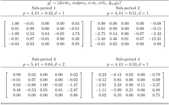
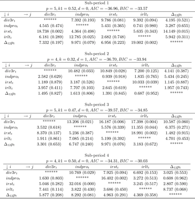
spherical disturbances. On a second run, among all these models, we select the one with the minimal AIC criterion (Akaike, 1974), and implement non-causality tests in this model. We report two kinds information: i) The estimates of the various long-term matrices A in Tables 5, 8 and 11, where the d variable signals if deterministic terms are added, where d = 1 means that an intercept is added, and d = 2 that an intercept plus a linear trend are included, and ii) The whole causal structure of the model. This allows analyzing if the long-term relations appear stable over time, as well as the stationarity of the variables, even if not formally tested. Speci…cations of the models are also presented. Tables (6), (9) and (12) present the results of non-causality tests for the di¤erent de…nitions of money.

Non-causality tests for DM4 Looking …rst at Table (5), it appears that the long term relationships change from a period to another, as the stationarity of the series. For instance, the long-term interest rate appears to be non-stationary in period 1 but stationary in sub-periods 2 and 3. Picking an other example, Divisia money is also integrated of order one in sub-periods 1, 2 and 3. The sub-periods 4 being hard to interpret due to the non-nullity of the cross-coe¤cicients. Turning to causality tests, Table (6), we fail to reject the null of non-causality from to money to activity in all sub-periods, whereas activity clearly granger-causes money in the last three periods. For sub-period 1, causality is found only at the 10 % threshold. Concerning the other causal relationships, unexpectedly, the short-term interest rate seems to play no driving role concerning activity, but appears to be a causal variable for money. At last, note that, except for few exceptions, the whole causal structure of the systems change from one period to another.

Non-causality tests for DM4- As previously noticed, here again, the …rst striking point is that the long-term matrices are period-dependent, Table (8). Turning to non-causality tests, Table (9), in all sub-periods, the null of non-causality from money to real activity is not rejected. In the same time, real activity Granger-causes money, but the results depend on the time-period considered. The null is accepted for sub-periods 1 and 3, and deeply rejected over periods 2, 4 and 5. Over these two latter periods, the short-term interest rate is the driving force of real activity. The relation between the interest rate and money is also not constant over time, and we reach a very similar conclusion as for DM4: the causal structures of the systems change over time.

(18)

Non-causality tests for DM3 Focusing now on DM3, and only on causality tests as presented in Table (12), we have the same patterns: On sub-period 1, we have no causal relationships between money and activity On sub-periods 2, 3 and 4, we reject non-causality from activity to money, while we fail to reject the null from money to activity.

Hence, whatever the de…nition of money used, the causal relationship for all models is clearly from activity to money, and not the converse.

4.3 Non-causality in surplus-lag VARX models

We next turn to results of non-causality tests in surplus-lag VARX models. Similarly to what we did for the FM-VAR lag selection, we use a double loop over p and p1, for p; p1 = 1; :::; 10, estimate the various ARX(p,p1) models, and keep those with spherical disturbances. In a second trial, among these models, we choose the one with the minimal AIC. Results are given by Tables (7), (10) and (13). We report the kind of model used, as well as the Wald statistic and the associated p-value, only for money and real activity.

Non-causality tests for DM4 Results using the broad monetary aggregate DM4, are similar with those obtained using the FM-VAR methodology. In sub-periods 2, 3 and 4 real activity is a causal variable of money. Results are less clear for sub-period 1 where causality is found only at the 10 % threshold. Interestingly, only in sub-period 2, the causal relation is bilateral, a result which is also suggested in Table (6).

Non-causality tests for DM4- Results are presented in Table (10). Concerning the null of non-causality from money to activity, it is accepted in all sup-periods. Focusing now on the causal relationship from activity to money it is clearly period-dependent, as within the FM-VAR framework: The null is rejected for sub-periods 2 and 5 (here at 10%), but accepted for other samples. Clearly, compared with DM4, the relationship is much more unstable.

Non-causality tests for DM3 At last, focusing on non-causality tests for DM3 returns ex-actly the same information as for tests implemented in FM-VAR models. For sub-period 1, no causal relationships are found between money and activity, whereas over other periods, the causal relationship is from activity to money. Hence, DM3 seems to behave as DM4.

(19)

5 Conclusion and discussion

In this paper, we have used Granger non-causality tests to investigate the empirical relationships between real money and activity. Three di¤erent broad measures of money as de…ned by the CFS have been used, DM4, DM4- and DM3. Tests have been implemented within two distinct frameworks: FM-VAR and surplus-lag VARX models. Results return important features: i) For all three aggregates, and for di¤erent sub-periods, tests suggest that if causality is found, it is from activity to real money, ii) In all models, there is no causal links between money and activity during the period January 1968 to July 1979, iii) For DM4-, the results are period-dependent, and the two aggregates showing a stable relationship with activity are the DM4 and DM3 ones, iv) From one sub-period to another, the whole causal structure of the systems, as well as the stationarity of some series seems to change, maybe also explaining the instability found previously by researchers, v) At last, the two methodologies return very similar information.

References

[1] Akaike, H. (1974) A New Look at the Statistical Model Identi…cation, IEEE Transactions on Automatic Control, AC-19, pp716-723.

[2] Anderson, R. and Rashce, R. (2001) Retail Sweep Programs and Bank Reserves, 1994-1999, Review, Federal Reserve Bank of St. Louis, January, pp 51-72.

[3] Andrews, D.W.K. (1991) Heteroskedasticity and Autocorrelation Consistent Covariance Ma-trix Estimation, Econonetrica 59, pp 817-858.

[4] Andrews, D.W.K. & J.C. Monahan (1992) An Improved Heteroskedasticity and Autocorre-lation Consistent Covariance Matrix Estimator, Econornetrica 60, pp 953-966.

[5] Bai, J. and P. Perron (1998) Estimating and Testing Linear Models with Multiple Structural Changes, Econometrica 66, pp 47–78

[6] Barnett, W. A.(1978). "The User Cost of Money." Economics Letter 1 145-149. Reprinted in William A. Barnett and Apostolos Serletis (eds.), 2000, The Theory of Monetary Aggre-gation, North Holland, Amsterdam, chapter 1, pp. 6-10.

[7] Barnett, W.A., 1980. Economic Monetary Aggregates: An Application of Aggregation and Index Number Theory, Journal of Econometrics 14, 11-48. Reprinted in William A. Barnett

(20)

and Apostolos Serletis (eds.), 2000, The Theory of Monetary Aggregation, North Holland, Amsterdam, chapter 1, pp. 6-10.

[8] Barnett, W.A., O¤enbacher, E. and P. Spindt (1981) New concepts of aggregated money, The Journal of Finance 36 pp. 497-505.

[9] Barnett, W.A., O¤enbacher, E. and P Spindt (1984) The New Divisia Monetary Aggre-gates, Journal of Political Economy 92, pp. 1049-1085. Reprinted in William A. Barnett and Apostolos Serletis (eds.), 2000, The Theory of Monetary Aggregation, North Holland, Amsterdam, chapter 17, pp. 360-388.

[10] Barnett, W.A., D. Fisher and A. Serletis (1992) Consumer Theory and The Demand for Money, Journal of Economic Literature 30, pp. 2086-2119.

[11] Barnett, W.A. and A. Serletis (2000) The Theory of Monetary Aggregation, Barnett, W.A. and A. Serletis eds. Elsevier, North Holland.

[12] Barnett, W.A., Chauvet, M. and H. Tierney (2009) Measurement Error In Monetary Ag-gregates: A Markov Switching Factor Approach, Macroeconomic Dynamics 13, pp 381-412. [13] Barnett, W.A. and P. de Peretti (2009): Admissible Clustering Of Aggregator Compo-nents: A Necessary And Su¢cient Stochastic Seminonparametric Test For Weak Separabil-ity Macroeconomic Dynamics 13, 317-334.

[14] Barnett, W.A., Liu, J., R. S. Mattson, and J. van den Noort (2012) The New CFS Divisia Monetary Aggregates: Design, Construction, and Data Sources, Manuscript. New York: Center for Financial Stability.

[15] Bauer, D. and A. Maynard (2012) Persistence-Robust Surplus-Lag Granger Causality Test-ing, Journal of Econometrics 169, pp 293–300

[16] Belongia, M.T. (1996) Measurement Matters: Recent Results From Monetary Economics Reexamined, Journal of Political Economy 104, 1065-1083.

[17] Belongia, M.T and J.M. Binner (2001) Divisia Monetary Aggregates Right in Theory, Useful in Practice: Theory and Practice, Michael T. Belongia and Jane M. Binner eds., London: Macmillan Press Ltd.

[18] Belongia, M.T. and P.N Ireland (2012a) The Barnett Critique After Three Decades: A New Keynesian Analysis, NBER Working Papers 17885.

(21)

[19] Belongia, M.T. and P.N Ireland (2012b) Quantitative Easing: Interest Rates and Money in the Measurement of Monetary Policy, working paper.

[20] Benati, L. and G. Kapetanios (2003) Structural Breaks in In‡ation Dynamics, ,Computing in Economics and Finance 169.

[21] Chan, N.H. (1988) The Parameter Inference for Nearly Nonstationary Time Series, Journal of the American Statistical Association 83, pp857-862.

[22] Chang, Y. (2000) Vector Autoregression With Unknown Mixtures of I(0); I(1) and I(2) components. Econometric Theory 16, 905-926.

[23] Chrystal, A. and MacDonald, R. 1994. Empirical evidence on the recent behaviour and usefulness of simple-sum and weighted measures of the money stock. Federal Reserve Bank of St. Louis Review 76, 73–109.

[24] Darrata, A.F., Chopinc, M.C. and Bento J. Lobo (2005) Money and Macroeconomic Per-formance: Revisiting Divisia Money, Review of Financial Economics 14, 93-101.

[25] de Peretti, P. (2007): Testing the signi…cance of the departures from weak separability. In Barnett, W.A. and A. Serletis (eds.), International Symposia in Economic Theory and Econometrics: Function Structure Inference, pp. 3-22. Amsterdam, Elsevier.

[26] Diebold, F.X. and A. Inoue (2001) Long Memory and Regime Switching, Journal of Econo-metrics 105, pp131-159.

[27] Diewert, W.E. (1976) Exact and Superlative Index Numbers, Journal of Econometrics 4, pp 115-145.

[28] Diewert, W.E. (1978) Superlative Index Numbers and Consistency in Aggregation, Econo-metrica46, pp. 883-900.

[29] Diewert, W.E. (1980) : Aggregation Problems in the Measurement of Capital, in The Mesurement of Capital, Dan Usher (ed.), University of Chicago Press.

[30] Dolado, J. and H. Lütkepohl (1996) Making Wald Tests Work for Cointegrated VAR Sys-tems, Econometric Reviews 15, pp 369-386.

[31] Dorich, J. (2009) Resurrecting the Role of Real Money Balance E¤ects, Bank of Canada Working Paper 2009-24

(22)

[32] Favara, G. and P.Giordani (2009), Reconsidering the Role of money for Output, Prices and Interest rates, Journal of Monetary Economics 56, pp 419-430.

[33] Feenstra, R. C. (1986): Functional Equivalence Between Liquidity Costs and the Utility of Money. Journal of Monetary Economics 22, 271-291.

[34] Fleissig, A. R. and G.A. Whitney (2003): New PC-Based test for varian’s weak separability conditions, Journal of Business and Economic Statistics 21, 133–144.

[35] Fleissig, A.R. and G.A. Whitney (2005): Testing the signi…cance of violations of Afriat’s inequalities, Journal of Business and Economic Statistics 23, 355-362.

[36] Granger, C.W.J. (1969) Investigating Causal Relations by Econometric Models and Cross-Spectral Methods, Econometrica 37, pp 424-438.

[37] Hayo, B. (1999) Money-Output Granger Causality Revisited: An Empirical Analysis of EU Countries, Applied Economics 31, 1489-1501.

[38] Ireland, P.N.(2004). Money’s Role in the Monetary Business Cycle Model, Journal of Money, Credit and Banking 36, pp 969-984.

[39] Muller, U.K. and M.W. Watson (2007) Low-frequency robust cointegration testing. NBER Working Papers 15292.

[40] O¤enbacher, A., and Shachar, S. (2011). Divisia Monetary Aggregates for Israel: Back-ground Note and Metadata. Bank of Israel, Research Department: Monetary/Finance Di-vision.

[41] Phillips, P.C.B. (1987) Towards a Uni…ed Asymptotic Theory for Autoregression, Biometrika 74, pp 535-547.

[42] Phillips, P.C.B (1995) Fully Modi…ed Least Squares and Vector Autoregression, Economet-rica63, 1023-1078.

[43] Phillips, P.C.B. (2005) Challenges of trending time series econometrics. Mathematics and Computer in Simulations 86, pp 401-416.

[44] Phillips, P.C.B, and B. Hansen (1990) Statistical Inference in Instrumental Variables Re-gression with I(1) Processes, Review of Economic Studies 57, pp 99-125.

(23)

[45] Poterba, J.M. and J.J. Rotemberg (1987): Money in the utility function: An empirical implementation. In New Approaches to Monetary Economics, eds. W. Barnett and K. Sin-gleton, Cambridge University Press, 219-240.

[46] Rahman, S. and A. Serletis (2012) The Case for Divisia Money Targeting, Macroeconomic Dynamics 16,pp 1-21.

[47] Saikkonen, P. and H. Lütkepohl (1996) In…nite-Order Cointegrated Vector Autoregressive Processes, Econometric Theory 12, pp 814-844.

[48] Schunk, D. (2001) The Relative Forecasting Performance of the Divisia and Simple Sum Monetary Aggregates, Journal of Money, Credit and Banking 33, pp. 272-283.

[49] Serletis, A. (1991) The Demand for Divisia Money in the United States : A Dynamic Flexible Demand System, Journal of Money, Credit and Banking 23, pp 35-52.

[50] Serletis, A. and M. King (1993).The Role of Money in Canada, Journal of Macroeconomics 15, pp 91-107.

[51] Sims, C.A. (1972) Money, Income and Causality, The American Economic Review 62, pp 540-552.

[52] Sims, C.A. (1980) Macroconomics and Reality, Econometrica 48, pp 1-48.

[53] Sims, C.A., Stock, J.H. and M.W. Watson (1990) Inference in Linear Time Series with Some Unit Roots, Econometrica 58, 113-144.

[54] Stock, H.J. and M.W. Watson (1989) Interpreting the evidence on Money-Income Causality, Journal of Econometrics 40, pp161-189.

[55] Swo¤ord, J.L. and G.A. Whitney (1987): Non-Parametric tests of utility maximization and weak separability for consumption, leisure, and money, Review of Economic Studies 69, 458–464.

[56] Swo¤ord, J.L. and G.A. Whitney (1988): A comparison of nonparametric tests of weak separability for annual and quarterly data on consumption, leisure, and money, Journal of Business & Economic Statistics 6, 241-246

[57] Toda, H.Y. and P.C.B. Phillips (1993) Vector Autoregression and Causality, Econometrica 61, pp 1367-1393.

(24)

[58] Toda, H.Y. and P.C.B. Phillips (1994) Vector Autoregression and Causality: A Theoretical Overview and Simulation Study, Econometric Reviews 13, pp 259-285.

[59] Toda, H.Y. and T. Yamamoto (1995) Statistical Inference in Vector Autoregressions with Possibly Integrated Processes, Journal of Econometrics 66, pp 225-250.

[60] Varian, H. (1983): Nonparametric Tests of Consumer Behavior, Review of Economic Studies 50, 99–110.

[61] Yamada, H. and H.Y. Toda (1997) A Note on Hypothesis Testing Based on the Fully Mod-i…ed Vector Autoregression, Economics Letters 56, pp 55-95.

[62] Yue, P. and R. Fluri (1991) Divisia Monetary Services Indexes for Switzerland : Are They Useful for Monetary Targeting?, Federal Reserve Bank of St Louis Review 73, pp 19-33. [63] Walsh, C.E. (2003) Monetary Theory and Policy 2nd edition, MIT press.

[64] Woodford, M.D.(2003). Interest and Prices. Princeton, New Jersey: Princeton University Press.

(25)

(26)

Table 5: Long-term matrices A for the four sub-periods. Money de…ned as div4rt

y1

t = (div4rt; indprot; irstt; irltt; 12pt)0

Sub-period 1 Sub-period 2 p = 4; k1 = 0:42; d = 1 p = 4; k1 = 0:51; d = 1 2 6 6 6 6 4 1:00 0:01 0:00 0:00 0:05 0:01 0:99 0:00 0:00 0:01 1:09 0:53 0:84 0:05 4:73 0:91 0:97 0:01 0:90 0:38 0:03 0:03 0:00 0:00 0:95 3 7 7 7 7 5 2 6 6 6 6 4 0:98 0:00 0:00 0:00 0:08 0:01 0:99 0:00 0:00 0:15 2:75 0:54 0:96 0:07 2:42 5:48 3:46 0:01 0:87 12:31 0:01 0:02 0:00 0:00 0:88 3 7 7 7 7 5 Sub-period 3 Sub-period 4 p = 5; k1 = 0:64; d = 2 p = 4; k1 = 0:53; d = 1 2 6 6 6 6 4 0:99 0:02 0:00 0:00 0:02 0:01 0:97 0:00 0:00 0:02 0:03 0:86 1:00 0:02 1:47 0:48 0:53 0:05 0:81 2:87 0:00 0:00 0:00 0:00 0:86 3 7 7 7 7 5 2 6 6 6 6 4 0:23 0:12 0:02 0:00 0:79 0:12 0:85 0:00 0:00 0:09 2:91 2:33 0:90 0:11 3:37 1:11 5:99 0:21 0:66 6:88 0:02 0:10 0:00 0:00 0:75 3 7 7 7 7 5

(27)

Table 6: FM-VAR causal structure. Non-causality from variable j in equation i. Main entries are the Wald statistics and the p-values (between parentheses)

Sub-period 1

p= 4; k1 = 0:42; d = 0; AIC = 37:41; BIC = 34:76

#i !j div4rt indprot irstt irltt 12pt

divrt ****** 9:339 (0:053) 2:667 (0:615) 8:001 (0:091) 4:243 (0:374) indprot 2:947 (0:566) ****** 5:742 (0:219) 0:456 (0:977) 1:840 (0:765) irstt 15:712 (0:003) 3:420 (0:490) ****** 1:425 (0:839) 5:222 (0:265) irltt 3:851 (0:426) 4:570 (0:334) 2:595 (0:628) ****** 3:239 (0:519) 12pt 3:643 (0:456) 14:311 (0:006) 8:770 (0:067) 18:793 (0:000) ****** Sub-period 2 p= 4; k = 0:51; d = 0; AIC = 34:57; BIC = 30:59

#i !j div4rt indprot irstt irltt ₁₂pt

divrt ****** 10:150 (0:038) 9:497 (0:049) 5:347 (0:235) 3:853 (0:426) indprot 9:143 (0:057) ****** 1:084 (0:896) 1:857 (0:762) 7:823 (0:098) irstt 4:672 (0:322) 0:935 (0:919) ****** 13:708 (0:008) 1:201 (0:878) irltt 6:879 (0:142) 7:296 (0:121) 1:106 (0:893) ****** 3:534 (0:473) 12pt 1:820 (0:768) 1:358 (0:851) 1:737 (0:783) 0:682 (0:953) ****** Sub-period 3 p= 5; k1 = 0:64; d = 1; AIC = 39:98; BIC = 36:84

divrt ****** 17:434 (0:004) 12:893 (0:024) 8:559 (0:128) 2:642 (0:754) indprot 8:647 (0:124) ****** 9:444 (0:093) 4:147 (0:528) 3:362 (0:644) irstt 1:803 (0:875) 17:691 (0:003) ****** 13:947 (0:016) 2:431 (0:787) irltt 3:103 (0:684) 3:613 (0:606) 17:441 (0:004) ****** 3:821 (0:575) 12pt 2:419 (0:788) 7:862 (0:164) 15:322 (0:009) 0:756 (0:981) ****** Sub-period 4 p= 4; k1 = 0:53; d = 0; AIC = 34:57; BIC = 30:59

divrt ****** 33:852 (0:000) 23:921 (0:000) 7:430 (0:115) 17:023 (0:002)

indprot 0:810 (0:937) ****** 6:864 (0:143) 4:300 (0:366) 0:511 (0:972)

irstt 9:664 (0:046) 32:042 (0:000) ****** 7:938 (0:094) 1:932 (0:748)

irltt 1:572 (0:813) 9:187 (0:056) 7:265 (0:122) ****** 5:035 (0:284) 12pt 11:601 (0:021) 6:851 (0:144) 2:047 (0:727) 4:748 (0:314) ******

(28)

Table 7: Non-causality tests in surplus-lag VARX models. Money de…ned as DM4 Sub-period 1

Model Dependent Variable Forcing Variable (Causal) Exogenous Control Variables Wald ARX(3,3) div4rt indprot irstt,irltt, 12pt 7.294 (0.063)

ARX(3,2) indprot div4rt irstt,irltt, ₁₂pt 0.128 (0.937)

Sub-period 2

ARX(3,3) div4rt indprot irstt,irltt, ₁₂pt 9.083 (0.028)

Sub-period 3

Sub-period 4

(29)

Table 8: Long-term matrices A for the …ve sub-periods. Money de…ned as div4mrt

y2

t = (div4rmt; indprot; irstt; irltt; 12pt)0

Sub-period 1 Sub-period 2 p = 5; k1 = 0:53; d = 0 p = 4; k1 = 0:56; d = 1 2 6 6 6 6 4 1:00 0:01 0:00 0:00 0:04 0:05 1:00 0:00 0:00 0:07 6:15 3:84 0:66 0:32 14:73 2:61 2:51 0:01 0:78 1:00 0:03 0:03 0:00 0:00 0:95 3 7 7 7 7 5 2 6 6 6 6 4 0:89 0:12 0:00 0:00 0:01 0:03 0:94 0:00 0:00 0:16 5:74 5:31 0:89 0:21 1:35 13:76 13:51 0:13 0:55 3:80 0:08 0:08 0:00 0:00 0:88 3 7 7 7 7 5 Sub-period 3 Sub-period 4 p = 4; k1 = 0:66; d = 1 p = 6; k1 = 0:38; d = 2 2 6 6 6 6 4 0:73 0:07 0:00 0:00 0:13 0:08 0:14 0:00 0:00 0:31 14:51 5:40 0:63 0:38 38:19 52:18 11:07 0:03 1:01 1:63 0:20 0:09 0:00 0:00 0:28 3 7 7 7 7 5 2 6 6 6 6 4 0:88 0:01 0:00 0:00 0:17 0:01 0:91 0:00 0:00 0:15 1:84 3:86 1:06 0:01 7:19 0:85 1:32 0:00 0:85 8:52 0:04 0:09 0:00 0:00 1:00 3 7 7 7 7 5 Sub-period 5 p = 4; k1 = 0:49; d = 1 2 6 6 6 6 4 0:99 0:02 0:00 0:00 0:02 0:01 0:97 0:00 0:00 0:02 0:03 0:86 1:00 0:02 1:47 0:48 0:53 0:05 0:81 2:87 0:00 0:00 0:00 0:00 0:86 3 7 7 7 7 5

(30)

Sub-period 1

p= 5; k1 = 0:53; d = 0; AIC = 36:85; BIC = 33:46

#i !j div4mrt indprot irstt irltt ₁₂pt

div4mrt ****** 8:094 (0:151) 8:413 (0:135) 9:763 (0:082) 3:085 (0:686) indprot 3:864 (0:569) ****** 5:722 (0:334) 0:756 (0:979) 2:832 (0:725) irstt 18:791 (0:002) 4:852 (0:434) ****** 6:055 (0:301) 13:697 (0:0176) irltt 7:205 (0:205) 14:268 (0:014) 2:721 (0:742) ****** 6:636 (0:249) 12pt 7:812 (0:166) 10:993 (0:051) 6:764 (0:238) 19:267 (0:001) ****** Sub-period 2 p= 4; k = 0:56; d = 1; AIC = 36:93; BIC = 33:79

#i !j div4mrt indprot irstt irltt 12pt

div4mrt ****** 32:972 (0:000) 29:359 (0:000) 23:865 (0:000) 7:307 (0:120) indprot 4:628 (0:327) ****** 1:395 (0:845) 0:880 (0:927) 6:607 (0:158) irstt 5:233 (0:264) 3:645 (0:456) ****** 14:925 (0:005) 1:230 (0:873) irltt 19:627 (0:000) 20:532 (0:000) 5:616 (0:229) ****** 0:802 (0:938) 12pt 10:521 (0:032) 8:931 (0:062) 11:699 (0:019) 9:021 (0:061) ****** Sub-period 3 p= 4; k1 = 0:66; d = 1; AIC = 39:29; BIC = 35:08

#i !j div4mrt indprot irstt irltt 12pt

div4mrt ****** 10:887 (0:027) 7:746 (0:101) 8:240 (0:083) 4:410 (0:353)

indprot 1:816 (0:769) ****** 15:805 (0:003) 2:134 (0:711) 0:344 (0:986)

irstt 6:384 (0:172) 41:646 (0:000) ****** 5:067 (0:280) 2:339 (0:373)

irltt 7:803 (0:099) 4:577 (0:333) 3:495 (0:478) ****** 8:925 (0:063) 12pt 6:085 (0:192) 9:969 (0:041) 3:243 (0:518) 4:143 (0:387) ******

(31)

Table 10: Non-causality tests in surplus-lag VARX models. Money de…ned as

DM4-Model Dependent Variable Forcing Variable (Causal) Exogenous Control Variables Wald Sub-period 1

ARX(2,2) div4mrt indprot irstt,irltt, ₁₂pt 4.389 (0.111)

ARX(6,2) indprot div4mrt irstt,irltt, ₁₂pt 0.238 (0.887)

Sub-period 2

Sub-period 3

Sub-period 4

Sub-period 5

Table 11: Long-term matrices A for the four sub-periods, money de…ned as div3rt

y3

t = (div3rt; indprot; irstt; irltt; 12pt)0

Sub-period 1 Sub-period 2 p = 5; k1 = 0:52; d = 0 p = 4; k1 = 0:32; d = 1 2 6 6 6 6 4 1:01 0:00 0:00 0:00 0:05 0:05 1:00 0:00 0:00 0:07 5:71 3:49 0:68 0:32 14:87 2:16 2:19 0:00 0:79 0:91 0:03 0:03 0:00 0:00 0:95 3 7 7 7 7 5 2 6 6 6 6 4 0:96 0:04 0:00 0:00 0:00 0:04 0:94 0:00 0:00 0:12 1:28 1:81 1:01 0:01 1:86 1:14 1:13 0:02 0:97 7:11 0:02 0:02 0:00 0:00 0:99 3 7 7 7 7 5 Sub-period 3 Sub-period 4 p = 5; k1 = 0:47; d = 0 p = 4; k1 = 0:50; d = 1 2 6 6 6 6 4 0:98 0:01 0:00 0:00 0:05 0:00 0:99 0:00 0:00 0:05 0:11 0:32 0:99 0:06 0:46 0:62 0:43 0:01 0:84 3:67 0:00 0:01 0:00 0:00 0:88 3 7 7 7 7 5 2 6 6 6 6 4 0:70 0:13 0:01 0:00 0:26 0:15 0:49 0:02 0:00 0:14 4:76 7:98 0:40 0:08 1:27 1:59 4:18 0:00 0:53 6:07 0:05 0:04 0:00 0:00 0:90 3 7 7 7 7 5

(32)

Sub-period 1

p= 5; k1 = 0:52; d = 0; AIC = 36:96; BIC = 33:57

div3rt ****** 7:392 (0:193) 9:786 (0:081) 9:392 (0:094) 4:195 (0:521) indprot 4:545 (0:474) ****** 5:431 (0:365) 0:741 (0:980) 3:287 (0:655) irstt 18:738 (0:002) 4:364 (0:498) ****** 5:635 (0:343) 14:149 (0:015) irltt 6:181 (0:289) 12:785 (0:025) 2:682 (0:748) ****** 5:942 (0:311) 12pt 7:332 (0:197) 9:971 (0:079) 6:956 (0:223) 19:002 (0:002) ****** Sub-period 2 p= 4; k = 0:32; d = 1; AIC = 36:70; BIC = 33:94

div3rt ****** 10:482 (0:033) 10:849 (0:028) 7:200 (0:125) 4:141 (0:387) indprot 2:582 (0:629) ****** 0:939 (0:918) 1:835 (0:765) 5:434 (0:245) irstt 1:189 (0:879) 3:187 (0:526) ****** 10:033 (0:039) 1:145 (0:887) irltt 3:957 (0:411) 7:707 (0:103) 2:645 (0:619) ****** 1:957 (0:743) 12pt 1:495 (0:827) 1:613 (0:806) 1:391 (0:845) 0:687 (0:952) ****** Sub-period 3 p= 5; k1 = 0:47; d = 0; AIC = 39:57; BIC = 34:85

div3rt ****** 13:206 (0:021) 16:187 (0:006) 17:398 (0:004) 10:587 (0:060) indprot 3:532 (0:618) ****** 5:576 (0:339) 11:355 (0:044) 6:375 (0:271) irstt 8:370 (0:137) 5:236 (0:387) ****** 18:991 (0:002) 1:482 (0:915) irltt 1:911 (0:861) 7:085 (0:214) 5:199 (0:392) ****** 4:701 (0:453) 12pt 3:301 (0:653) 6:747 (0:240) 9:971 (0:076) 3:183 (0:672) ****** Sub-period 4 p= 4; k1 = 0:50; d = 0; AIC = 34:31; BIC = 30:03

div3rt ****** 10:769 (0:029) 7:925 (0:094) 6:692 (0:153) 3:025 (0:553)

indprot 1:630 (0:803) ****** 16:402 (0:002) 3:272 (0:513) 0:608 (0:962)

irstt 5:046 (0:282) 32:016 (0:000) ****** 3:245 (0:517) 2:807 (0:590)

irltt 7:441 (0:114) 3:822 (0:430) 3:686 (0:450) ****** 8:737 (0:068) 12pt 5:877 (0:208) 8:292 (0:081) 4:963 (0:291) 4:369 (0:358) ******

(33)

Table 13: Non-causality tests in surplus-lag VARX models. Money de…ned as DM3 Sub-period 1

Model Dependent Variable Forcing Variable (Causal) Exogenous Control Variables Wald ARX(2,2) div3rt indprot irstt,irltt, 12pt 3.998 (0.135)

Sub-period 2

Sub-period 3

Sub-period 4