HAL Id: halshs-00335025
https://halshs.archives-ouvertes.fr/halshs-00335025
Submitted on 28 Oct 2008HAL is a multi-disciplinary open access archive for the deposit and dissemination of sci-entific research documents, whether they are pub-lished or not. The documents may come from teaching and research institutions in France or abroad, or from public or private research centers.
L’archive ouverte pluridisciplinaire HAL, est destinée au dépôt et à la diffusion de documents scientifiques de niveau recherche, publiés ou non, émanant des établissements d’enseignement et de recherche français ou étrangers, des laboratoires publics ou privés.
Prices and output co-movements : an empirical
investigation for the CEECs
Iuliana Matei
To cite this version:
Iuliana Matei. Prices and output co-movements : an empirical investigation for the CEECs. 2008. �halshs-00335025�
Documents de Travail du
Centre d’Economie de la Sorbonne
Maison des Sciences Économiques, 106-112 boulevard de L'Hôpital, 75647 Paris Cedex 13 http://ces.univ-paris1.fr/cesdp/CES-docs.htm
ISSN : 1955-611X
Prices and output co-movements : an empirical investigation for the CEECs
Iuliana MATEI
Prices and output co-movements: an empirical investigation for the CEECs
Iuliana Mateiϯ
October 21, 2008
Abstract: This article studies the features of co-movements of prices and production between six CEECs recently joined the EU and the euro zone. More precisely, based partially on the methodology suggested by Alesina, Barro and Tenreyro [2002], we evaluate the size and the persistence of prices and outputs shocks between each CEECs and euro zone. Results will contribute to the debate around the participation of the new members to the EMU.
Key-words: European monetary integration, co-movements, AR models, CEECs
Résumé: Cet article étudie les particularités des co-mouvements des prix et production entre d’une part, six PECO récemment intégrés dans l’UE et d’autre part, la zone euro. Plus précisément, à l’aide d’une méthodologie suggérée par les travaux d’Alesina, Barro et Tenreyro (2002), nous évaluons la taille et la persistance des chocs des prix et production entre les PECO et la zone euro. Nos résultats tentent de contribuer aux débats sur la participation des nouveaux entrants dans l’union monétaire européenne.
Mots-clés: Integration monétaire européenne, co-mouvements, modèles AR, PECO JEL Classification : C22, E30, F33, F42, F47.
We are grateful for suggestions from Peter Howitt, Mathilde Maurel and Sandra Poncet as well as seminar participants at University of Paris 1 comming from TEAM and ROSES, conference organizers and participants of the Jerusalem Summer School in Economic Growth, 5th EUROFRAME Conference on Economic Policy Issues in the European Union, Monetary and Financial Transformations in the CEECs, Journées de l’AFSE: Développement récents en Economie Financière, aspects microéconomiques et macroéconomiques, Reaserch in International Economics and Finance, Vth International Seminar of the Young Phd Students in Economic Integration and Exchange rate econometrics. The errors and omissions which could remain are of course of our only responsability.
ϯChercheur Associé au Centre d’Economie de la Sorbonne, Université Paris 1 Panthéon-Sorbonne, 106-112, Bd. de l'Hôpital, Paris 75013, France. Email:iuliana.matei@malix.univ-paris1.fr.
1 Introduction
From 1st January 2007, the European Union counts 27 member states. Ten CEECs (Bulgaria, Czech Republic, Estonia, Hungary, Latvia, Lithuania, Poland, Romania, Slovak Republic and Slovenia) along with Cyprus and Malta have joined the 15 older EU members. Following the
largest expansion in its history, 27 countries must now strive to respect the acquis communautaire1
especially in terms of single currency project and to integrate their national structures and their citizens on a scale never seen before.
This recent enlargement of EU raises essential questions particularly around the participation of the new members to the EMU. Due to their progress during a still unfinished transition and convergence process, the new EU states have as objective to join euro zone for some reasons: this entry could guarantee them lower interest rate, a certain monetary stability and a more easily access to foreign founds. Contrary to the case of Denmark and the United Kingdom in 1999, they can not beneficiate of the opt-out clause. Consequently, they have to prepare their accession to Euroland as soon as possible in agreement principally with the Maastricht criteria. The accession to euro zone and its effects became consequently a crucial key issue for their future. The entry into a monetary union involves both costs and benefits for member countries. The costs of the adoption of a common currency are generally established according to two criterions: (i) institutional criterion (Maastricht convergence criteria) and (ii) criteria derived from the theory of optimal currency areas (OCA) initiated by Mundell (1961), McKinnon (1963) and Kenen (1969). If the Maastricht treaty privileges criterions of nominal convergence to evaluate the practical feasibility of the euro area and the risks weighing on the independence of the European Central Bank, the OCA criterions emphasize structural criterions such as those related to the benefits of a monetary union: two countries or areas will profit from a monetary union if they are characterized by a great similarity of the business cycles, have strong commercial linkages and a mechanism to mitigate the negative effects of the asymmetrical shocks. It is worth noting that the most commonly identified cost in the theoretical and empirical literature is the loss of monetary policy as national stabilization tool and the most cited benefit of a monetary union is the increase in trade and foreign investments. Beyond these various structural criteria of OCA theory which can guide in the choice of the exchange rate regimes, an important role plays the
1
nature of the shocks affecting a monetary area. In the case of the symmetrical shocks affecting the economies, the fixed exchange rate regimes are preferable compared to their flexibility. In the case of asymmetrical shocks, the opposite situation has to be taken into account: a more flexibility of the exchange rate regimes. But, perfectly symmetrical shocks don’t exist. Because of this raison, the most part of the literature focuses on the degree of shocks symmetries rather than the nature of the shocks. Hence, the principal idea of this approach is that costs of a monetary union decrease proportionally with the degree of symmetry of the shocks (i.e, the business cycles should be synchronized when the currencies are anchored to the euro because of the existence of a common monetary policy).
The empirical literature on the nature and the degree of the shock’s symmetries exploit usually descriptive statistics, econometric estimates or stochastic simulations. The descriptive statistics focuses on the correlations between the representatives economic variables such as the GDP growth, variability of cyclical components of industrial production etc. and consider that a strongly positive correlation of the cyclical components implies the existence of the shocks mainly symmetrical. These methods ignore the structural changes and don’t distinguish between the shocks and the answer to the shocks. Concerning the econometric estimates, the majority of studies uses as econometric method a structural VAR model developed by Blanchard and Quah (1989) and Bayoumi and Eichengreen (1993, 1996) to study both the supply and demand shocks affecting the EU members and their degree of (a)symmetry. Finally, the stochastic simulations are based on an econometric model in which the residuals are compared to macroeconomic shocks. These studies estimate a model drawing randomly from the shocks in the estimated distributions and compute then the variance of the different representative variables (production, prices) entering in these functions (Masson and Symansky, 1992). Other methods could be used to analyze the nature of shocks and the degree of shocks asymmetries such as the co-movements features for representative economic variables (Alesina, Barro and Tenreyro, 2002).
The focus of this paper is to analyze the characteristics of production and prices co-movements between each new EU member states and euro zone using partially the methodology developed by Alesina, Barro and Tenreyro [2002]. To our best knowledge, it was never tempted to provide an investigation of the co-movements in the case of the new EU member’s states. According to Alesina, Barro and Tenreyro [2002] approach, a positive response of the co-movements to the monetary union would lead to a higher degree of consensus around a common monetary policy without involving imbalances between participants and to lower costs generated by the loss of the monetary autonomy. A negative response of the co-movements would have the opposite
effect: it would generate divergent fluctuations and in this case, the exchange rate policies will be crucial to support the economic activity. Remarkably little attention has been paid to methods for measuring the co-movements, principally, in the case of new member states. In this sense, Alesina, Barro and Tenreyro [2002] approach exploit one of the various sensitivity indices – the conditional variance - to measure the co-movements. From the methodological point of view, the purpose of this paper is to examine the co-movements by exploiting recently new class of so-called variance-based sensitivity indices: the conditional variance and, respectively, the unconditional variance. The two concepts are very different, as illustrated for example in studies of inflation, in which the unconditional variance simply measures inflation variability, while the conditional forecast error variance measures inflation uncertainty (see, for example, Ball and Cecchetti, 1990). In its basic form, the link between these two concepts is highlighted by the law of total variance and can be expressed by " varY – E[varY|X] " as sensitivity index which is the "unconditional variance minus expected conditional variance of Y given parameter X" and may be interpreted as the "amount of the variance of Y that is expected to be eliminated if the true value of parameter X will become known". These methodological contributions lead to results suggesting that price co-movements are higher than production co-movements and that, generally, they are closed to those of the former EU member states. Our contribution is twofold. Firstly, we concentrate our attention on the recent experience of the new EU member states which are interesting examples to evaluate the prices and outputs co-movements in the ex-ante conditions (i.e., before entering into EU): countries characterized by the heterogeneity of the exchange rate regimes, recently integrated into EU and candidates for the adoption of the euro. Secondly, from the methodological point of view, we provide an additional test of the Alesina, Barro and Tenreyro [2002] approach to study the co-movements. More precisely, in the general framework of the autoregressive models, we carried out this analysis using both sensitivity indices: the conditional variance and the unconditional variance to point out business cycles synchronization.
The remainder of the paper is as follows. The next section reviews the literature on the costs and the benefits of a monetary union focusing on the new EU member’s case. Section 3 present some stylized facts related to the shocks symmetries. Section 4 details the empirical methodology and data sources. Section 5 reports the main results of our empirical model and discuss them. Section 6 offers the conclusions.
2 Literature review
The empirical literature around the costs and the benefits of a monetary union is relatively recent. We can distinguish two large approaches: the first investigating the occurrence of the asymmetric shocks between the old and the new members of EU and the second, focusing on the effects of a monetary union on the trade linkages. To have a coherent outline, we propose to present briefly a review of the empirical literature on the costs and the benefits of a monetary union in the CEECs context with a particular focus on the research about the shocks (a)symmetries.
Concerning the first approach, the recent studies on the shocks (a)symmetries between the old and the new EU member states become numerous after the adoption of the Maastricht treaty which maked credible the idea of the European Monetary Integration. The most part of these studies use as econometric method a structural vector autoregressive model (VAR model) developped initially by Blanchard and Quah (1989) and Bayoumi and Eichengreen (1993, 1996) in order to analyse the supply and demand shocks affecting the EU countries and their degree of asymmetry. Frenkel, Nickel and Schmidt (1999) and Horvath and Ratfai (2004) show that neither the correlation of the supply shocks or demand shocks make it possible to conclude in favor of the convergence for European countries. Fidrmuc and Korhonen (2001) highlight a certain heterogeneity concerning the correlation of the supply shocks between the EU and CEECs. The correlation of the demand shocks appears significant for Estonia and Hungary, while for the other CEECs, the results of the estimates seem to be non-significant. Babetski, Boone and Maurel (2002, 2004) widen the analysis of the supply and demand shocks by measuring the correlation in time starting from the methodology of Boone (1997). Their results show a process in course of convergence of the demande shocks between the EU and its new members while the supply shocks tend to diverge because of the transition process and the Balassa-Samuelson effect. In the general framework of the structural VAR, Frenkel and Nickel (2002) identify and compare demand and supply shocks between euro area countries and CEECs. Compared to Babetski, Boone and Maurel (2002, 2004) which use data since 1990 (corresponding to falls of the productions during the transition process to market economy), Frenkel and Nickel (2002) use more recent data (1993-2001) and thus, less affected by the structural shocks. Their analysis shows that there are still differences in the shocks and in the process of adjustment to shocks between the euro area and CEECs. But, they find also some similarities with euro area countries for several individual CEECs. Boone and Maurel (1999) study the date for which it would be optimal for CEECs to form a monetary union with Germany or with EU. Using the methodology of Reichlin and Forni (1997) and Fuss (1997) and using data over the period
1991-1997 for four CEECs, they find that the correlations of industrial production and unemployment cycles in the CEECs and the EU, point towards a deeper integration of the CEECs with Germany than with the EU. They also emphasise that pegging the currencies is a good policy option for CEECs. Alesina, Barro and Tenreyro (2002) study the comouvements of prices and outputs for various countries compared to the euro, the dollar and the yen and identify the „natural” OCA for these three monetary anchors. They use data on inflation, trade and prices and output co-movements over the period 1960 - 1997. Their results show that there exist monetary areas well defined by the dollar and the euro - as potential monetary anchors, but not defined by the yen. They highlight that pegging the currencies to euro and dollar increases the bilateral commercial linkages and the price co-movements and note that both prices and output co-movements don’t appear systematically corelated. In the same vain with Frankel and Rose (1998) approach, they argue that co-movements in „ex-ante” conditions could under-estimate the potential benefits of integration into a monetary union.
Another group of papers focus on the links between exhange rate regimes and the performances in terms of inflation in the case of EU countries. Borghijs and Kuijs (2004) analyze the costs and the benefit generated by the loss of the monetary autonomy which depends on the nature of the asymmetrical shocks striking an economy and on the capacity of the exchange rate regimes to absorb these shocks. Using a structural VAR model for five CEECs (Czech Republic, Hungary, Poland, Slovakia and Slovenia), their results suggest that the exchange rate chanel seems to be more important as propagator of the monetary and financial shocks than as an effective absorber of the real shocks. Coricelli, Jazbec and Masten (2003) analyze the link between the exchange rate regimes and the performances in terms of inflation for four CEECs: Czech Republic, Hungary, Poland and Slovenia and find that a fast adoption of the euro could provide a more effective framework to reduce inflation. In the same line, Goldfajn and Werlang (2000) analyze the relation between the depreciation of the exchange rate and the inflation for 71 countries between 1980-1998 while Darvas (2001) analyze the same problematic over the period 1993 -2000, but, in the case of four CEECs (Czech Republic, Hungary, Poland and Slovenia).
The second approach focus on the effects of the monetary union on the trade. Recent papers have questioned on this problematic such as: Artis and Zhang (1995), Frankel and Rose (2002, 1996), Rose (2000), Engel and Rose (2001), Alesina, Barro and Tenreyro (2002), Glick and Rose (2001), Flandrau and Maurel (2001) etc.. Artis and Zhang (1995) show that during the 80s and 90s, parallel to a better integration in Europe, the degree of correlation of the business cycles economies increased. Frankel and Rose (2000) estimate the effects of the monetary unions on the
trade and the production by using economic and geographical data for 200 countries. Their results reveal that the positive effects of the monetary unions on the macroeconomic performances of each country are rather due to the trade likages than to an adoption of a common monetary policy or to other types of macroeconomic influence. Frankel and Rose (1996) also analyze the impact of the intensity of the commercial links on the bilateral economic activity and conclude that a more intense commercial link is strongly associated with a high correlation of the economic activities. These authors highlight a negative correlation between the degree of (a) symmetry of the shocks and the trade integration.
Finally, a large empirical literature has investigated the shocks persistence in macroeconomics. This analysis becomes popular in macroeconomics with Nelson and Plosser [1982] insights about the stochastic trends. More precisely, they demonstrate that the real gross domestic product follows a unit root model. Other developments have succeeded around this problematic: Cochrane [1988], Rudebusch [1993], Macaro [2007] which argue that the presence of a unit root in the real gross domestic product is uncertain. A much smaller literature (Babetski, Boone and Maurel (2002, 2004), Boone and Maurel (1999)) led to a long and fruitful interlude in the development of ideas about economic fluctuations and about methods to be used for the analysis of these fluctuations in the CEECs context.
3 Some stylized facts
A manner to study the degree of (a) symmetry of the shocks is to compare the business cycles between CEECs and euro zone or EU. Our purpose in this section is to analyze some properties of the business cycles for two important macroeconomic variables. The variables considered are the industrial production (as proxy of GDP) and the consumer price index. In appendix, the tables from 8 to 12 expose the business cycles correlation between EU countries and euro zone. The results are presented at the same time over the whole period 1994-2004 and on the sub-periods (1994-1998 and 1999-2004). It should be noted that the series were broken up using the Hodrick Prescott filter to extract the trend and the cycle. Concerning the industrial production, we note that the business cycles of the CEECs appear more or less correlated with that of the euro area. Compared to the other CEECs, only Slovenia is correlated with the euro area at the same time on the sub-periods and on the whole period. Its business cycle is correlated more with euro area cycle for the sub-period 1999-2004 than on the whole period because of the transition process to the market economy (0.51 for 1999-2004 and 0.41 for 1994-1998). This observation
underlines the advantages or the disadvantages related to the possibility to enter into euro zone. These results incline the balance rather in favour of an integration in the euro zone for Slovenia. Concerning the prices evolutions, the CEECs fluctuations are very correlated (except for Slovakia) with those of the euro area particularly on 1999-2004. This fact could be justified by the price stability objective or targeting inflation strategy to join the EU in 2004. We observe that the CEECs correlations of business cycles with the euro area are different between countries: from 0.73 for Estonia or 0.70 for Slovenia to 0.01 for Slovakia on the sub-period 1999-2004. It will be interesting to see if the same results are obtained if we use the co-movement approach.
4 Methodology and data sources
The modern economies are closely dependent through the trade, the monetary and financial flows and the investments and consequently, events occurring in a country can have effects on other countries. The recent developments on the international transmission of the fluctuations concentrate at the same time on connections between these various countries and on the impacts that those could have on the transmission of the fluctuations. In the academic research, this aspect is studied in terms of volatility and co-movements in the macroeconomic series between country or regions. Even though they cannot claim to be precise, econometric models to estimate co-movements offer quantitative information which merits considerable attention and answer questions about the possible cyclical features of the evolution of economies to which they apply.
4.1 Methodology
We estimate a model which combines insights from Alesina, Barro and Tenreyro [2002, ABT], Cochrane [1988] and Ball and Cecchetti [1990]. As evidenced by ABT [2002] approach, the price equation corresponding to a pair of countries (i,j) is given by:
ln Pit/Pjt= f0+ f1ln Pi,t-1/Pj,t-1 + f2ln Pi,t-2/Pj,t-2 + εtij. (1)
where Pit/Pjt represent the price level in country i (i.e., one of the CEECs) relative to that in the
euro zone noted with j. For each pair of countries, (i, j), we compute then the second order autoregression presented above on quarterly data using the consumer price index. The estimated
residual êt, i, j measures the relative prices that can not be predictable from the two prior values of
VPij= √(1/T-3)∑(êijt)2 where T = the number of observations which is 37. (2)
We note that the co-movements are defined using the conditional variance (var xt|xt-1 Λ xt-2)
which take into account the passed values of our series xt (where xt = ln Pit/Pjt). We can observe
that the lower VPij, the greater the co-movement of prices between countries i and j and
therefore, the costs of a monetary union should be lower than the benefits. It is worth noting that, if both series are affected by symmetric shocks, the conditional variance of the ratio of the series should be near to zero.
The same method is applied to compute a measure of output co-movement (VYij) using the
similar concept: the conditional variance. For each pair of countries, (i, j), the value VYij comes
from the estimated residuals from the second order autoregression on quarterly data for industrial production:
ln (Yit/Yjt) = g0+g1ln (Yi,t-1/Yj,t-1) +g2ln (Yi,t-2/Yj,t-2) + utij. (3)
In the same vain, the estimated residuals ûtij measure the outputs that can not be predictable from
their two prior values. Using the root-mean-squared error, we compute analogously the output
co-movement VYij:
VYij= √(1/T-2)∑( ûijt)2 where T = 37 (4)
The conditional variance constitutes one of the various indices of sensitivity (also called indices of "uncertainty importance") used by ABT [2002] approach to measure the co-movements. In this paper, we contribute to the extent of co-movements by using another variance index such as the unconditional variance. The unconditional variance can be defined as the variance that don’t
take into account the passed values of our series xt = lnPit/Pjt and provides a best prediction on
the autoregressive process. If the unconditional variance refers to the variability of the macroeconomic series, the conditional variance concerns principally their predictability. According to the law of variance decomposition, the difference between unconditional variance (i.e, the variance of changes in inflation for example) and the conditional variance (i.e, the variance of unanticipated changes in inflation) offer the complementary part of the total variance and may be interpreted as the “amount of the variance of x that is expected to be eliminated
given the past values of x2. This strategy supposes to compute the co-movements using the
results obtained before. The price co-movement takes then the following form (see appendix): 2Several findings in the literature (Ball and Cecchetti, 1990) highlight that the inflation-uncertainty relation
across countries differs from the relation over time in a given country. Across countries, short-term as well as long-term uncertainty rises with average inflation. Finally, the inflation-uncertainty relation in
VPij (1 - Φ2) (5)
VP*ij=
(1 + Φ2) (1 - Φ2 – Φ1 ) (1 - Φ2 + Φ1)
where VP = var(εtij), VP*ij = var(xt), xt = lnPit/Pjtand the denominator different from zero.
Finally, the production co-movement obtained using the unconditional variance is given by the following expression:
VYij (1 - Φ2) (6)
VY*ij= (1 + Φ2) (1 - Φ2 – Φ1 ) (1 - Φ2 + Φ1)
where VY = var(εtij), VY*ij = var(xt), xt = ln Yit/Yjt and the denominator different from zero.
4.2 Data sources
Data on production and prices come from the IFS - International Financial Statistics and Eurostat. Combining both sources, we form a panel of countries with quarterly data on outputs and prices from 1995:01 to 2004:01 (i.e, before their accession into EU). For production, we use industrial production index and for prices, the consumer price index with 2000=100. To motivate our own stochastic model, we perform a preliminary analysis of CEECs using data for 1994:01-2004:04. We compute then simple measures to analyze the correlation of business cycles using industrial production index and the consumer price index. .
5 Results
This section presents our main empirical findings. We estimate our models and look at the relation between the co-movements obtained with both methods. We analyze these relations across countries: for some former EU members and new EU members states. The study of shocks persistence suppose to test the existence of unit roots in the macroeconomic series using different unit roots procedures such us: Augmented Dickey Fuller test (ADF test, 1981) and the Kwiatkowski, Philips, Schmidt and Shin (KPSS test, 1992). The KPSS test (1992) which has
countries with very high inflation is similar to the relation in moderate-inflation countries, though somewhat stronger.
stationarity under its null is used for confirming or cancelling ADF tests results and is performed with a Bartlett kernel where the bandwidth parameter is selected using the Newey and West (1994) automatic parameter method. Both procedures are applied to check whether they fit the data. Our estimates indicate that output and prices series follow an AR (2) model. Thus, series are non-stationary in level and have unit roots. A large part of the existing empirical literature on the EU countries has indicated that the euro zone series are less volatile than the national series. The results reported below on the relative size of shocks between CEECs and euro zone will be useful to fit this kind of comparisons.
The second column of tables 1 and 2 shows the results on co-movements using the conditional variance using the ABT method. The third column presents the co-movement using the un-conditional variance. The last method has the advantage that it takes into account the volatility of the permanent component (the trend) which is propriety of all autocorrelations. This issue is important because the conventional procedures (ADF procedure) focus usually on the first correlations to fit the short dynamic of the macroeconomic series and sometimes there is a risk of spurious regressions. But, what is important is that the residuals from the regressions (1) and (3) capture the unanticipated changes in relative prices or in the output differentials between the new members and the former members (i.e, the part not predictable from the two prior members of each equation noted above). By computing the co-movements using the conditional variance and the unconditional variance, we measure the relation between variability and the uncertainty of relative prices or output differentials. As one can observe, the results suggest that the uncertainty- variability distinction is not so important in all computations.
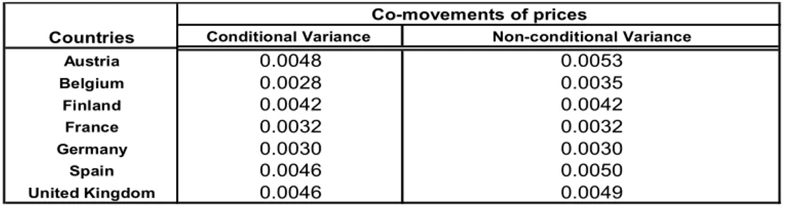
Concerning the new EU member states, the results of the table 1 and 2 show that the co-movements of prices are higher than the co-co-movements of outputs and that they are not systematically correlated. In the other hand, the co-movements of prices of the CEECs are lower than the co-movements of prices of the former EU and euro zone. The smallest co-movement of price is that of the Slovak Republic (0.131 in both cases of the variance indices) follow by the co-movement of the Czech Republic (0.0083 or 0.0087). The price’s co-co-movements of Estonia (0.0069) and Slovenia (0.0062) are closer to those of the former EU member’s states which are between 0.0030 and 0.0048. The prices co-movements for the Poland (0.0073 or 0.0084) and Hungary (0.0071 or 0.0084) are much closer in terms of the conditional variance. For these countries, the difference between both variance indices is larger than in the case of the other CEECs of our sample.
Table 1. Co-movements of relative prices for six CEECs
Conditional Variance Non-conditional Variance
Czech Rep. 0.0083 0.0087 Estonia 0.0069 0.0070 Hungary 0.0071 0.0084 Poland 0.0073 0.0076 Slovak Rep. 0.0131 0.0131 Slovenia 0.0062 0.0062 Countries Co-movements of prices
Table 2. Co-movements of production for six CEECs
Conditional Variance Non-conditional Variance
Czech Rep. 0.0277 0.0280 Estonia 0.0279 0.0289 Hungary 0.0207 0.0208 Poland 0.0260 0.0266 Slovak Rep. 0.0305 0.0307 Slovenia 0.0203 0.0236 Countries Co-movements of production
The Tables 3 and 4 present the results of our estimations in the case of the former EU countries. These results are closed to those obtained by ABT [2002] for some EU members between 1960 and 1997 (see tables 5 and 6 in appendix) using annual data.
Table 3. Co-movements of prices for some former EU members
Conditional Variance Non-conditional Variance
Austria 0.0048 0.0053 Belgium 0.0028 0.0035 Finland 0.0042 0.0042 France 0.0032 0.0032 Germany 0.0030 0.0030 Spain 0.0046 0.0050 United Kingdom 0.0046 0.0049 Countries Co-movements of prices
Table 4. Co-movements of production for some former EU members
Conditional Variance Non-conditional Variance
Austria 0.0175 0.0200 Belgium 0.0189 0.0267 Finland 0.0226 0.0252 France 0.0167 0.0213 Germany 0.0226 0.0342 Spain 0.0158 0.0239 United Kingdom 0.0157 0.0190 Countries Co-movements of production
We observe that the output co-movements for CEECs are closed to the co-movements of some countries of euro zone like: Germany, Belgium or Finland. These results are similar to those obtained by ABT [2002] for Norway (0.0210) or Cyprus (0.0227). Again the co-movement of
production of the Slovak Republic (0.0305 or 0.0307) followed by the production co-movements of the Czech Republic (0.0277 or 0.0280) are smaller than the other CEECs co-movements which suggest higher costs for abandoning the monetary policy. In other words, their output co-movements imply that there are still differences in the level of production with euro zone because of the transition process or the Balassa Samuelson effect. It should be noted that the existence of the conditional convergence in terms of output between CEECs and euro zone should imply that the new member states should beneficiate of the same economic and political context which suggest a capacity to reform the institutions independently of the level of richness. In contrast, the concept of the unconditional convergence imply that the convergence between regions or countries should be favoured by cultural homogeneity, capital and employment mobility, specific budgetary redistribution to each country etc.
Concerning the prices movements, we can argue that they are higher than the output co-movements and tend to be closed to those of EU_15 countries. We have also to emphasize that both types of co-movements (output and prices co-movements) aren’t systematically correlated which is in line with the ABT results for some European countries for the period 1960-1997.
6 Conclusions
The focus on this article was double: to provide new estimates about the co-movements of prices and output between CEECs and euro zone before the entry of these countries into EU using two methods and to compare them afterwards with the results obtained for the former members of EU between 1960 and 1997 by ABT researchers. Based on this analysis, we find in the same line with ABT research that the co-movements of prices are higher than the co-movements of production in the CEECs case and they are not systematically correlated. The co-movements of production are much closed to the production co-movements of some Euro zone members which involve lower costs to accession. On the other hand, the prices co-movements of CEECs are lower than the prices co-movements of the former members of EU. It should be interesting to study in a future empirical research the characteristics of the co-movements after the entry of CEECs in EU in order to see if our results would underestimate the potential benefits from joining a currency union (as emphasized also by Rose (1996) and ABT (2002)).
References
Alesina A., Barro R., Tenreyro S. (2002), “Optimal currency areas“, NBER WP 9072, June. Artis M., Zhang W. (1995), “International Business Cycles and the ERM : Is there a European
Bussiness Cycle?“, CEPR Discussion Paper, n° 1191, August.
Babetskii I., Boone L., Maurel M. (2002, 2004), “Exchange Rate Regimes and Supply Shocks Asymmetry: the case of the Accession Countries”, CEPR Discussion Paper, DP3408, June.
Ball L, Cecchetti S.G. (1990) „Inflation and Uncertainty at Short and Long Horizons”, Brookings Papers on Economic Activity, Vol. 1990, No. 1 (1990), pp. 215-254.
Blanchard, O.J., Quah, D. (1989), “The Dynamic Effects of Aggregate Demand and Supply Disturbances“, American Economic Review, September, p. 655-673
Bayoumi, T., Eichengreen B. (1996), “Operationalizing the Theory of Optimum Currency Areas“, CEPR Discussion Paper, n° 1484.
Bayoumi, T., Eichengreen B (1993), “Shocking Aspects of European Monetary Unification”, NBER Working Paper, WP/No. 3949.
Boone, L., Maurel, M. (1999), « L’ancrage de l’Europe Centrale et Orientale à l’Union Européenne», Revue Economique, vol. 50, N° 6, novembre 1999, p. 1123 – 1137.
Boone L. (1997), “Symmetry and asymmetry of Supply and demand Shocks in the European Union: a Dynamic Analysis”, Working Paper 9703, CEPII
Borghijs A., Kuijs L. (2004), “Exchange Rates in Central Europe : A Blessing or a Curse?”, IMF Working Paper, WP/04/2.
Cochrane J. (1988), “How big is the random walk in GNP?”, Journal of Political Economy, 96 (1988), pp. 893–920.
Coricelli F., Jazbec B., Masten I. (2003), “Exchange Rate Pass-Through in Candidate Countries“, CEPR Discussion Paper n° 3894.
Darvas Z. (2001), “Exchange Rate Pass-Through and Real Exchange Rate in EU Candidate Countries”, Deutsche Bundesbank Discussion Paper n°10.
De Grawve, P. (1997),“The Economics of Monetary Integration”, Oxford University Press. Deutsch Bank Research Note 99-04.
Engel, C. M, Rose, A. K. (2001). "Currency Unions and International Integration," CEPR Discussion Papers 2659, C.E.P.R. Discussion Papers
Flandreau, M., Maurel M. (2001), “ Monetary Union, Trade Integration and Bussiness Cycles in 19th Century Europe: Just do it “ , CEPR Discussion Paper No. 3087.
Frankel, J.A, Rose, A. K (2000). "An Estimate of the Effect of Currency Unions on Trade and Output," CEPR Discussion Papers 2631
Frankel J., Rose A. (1996), ”Currency Crashes in Emerging Markets : An Empirical Treatement”, Journal of International Economics 3, vol. 41, pp. 351-366.
Frenkel M., Nickel C., Schmidt G. (1999), “Some Shocking Aspects of EMU Enlargment”, Frenkel M., Nickel C., (2002), “How symmetric are the shock Adjustment Dynamics Between
the Euro Area and the Central and Eastern European Countries?”, IMF WP 02/222. Hàrvath J., Ratfai A. (2004), “Supply and Demand Shocks in Accession Countries to the
Gil-Alana, L., Robinson, P.M., (1997) “Testing of unit root and other nonstationary hypotheses in macroeconomic time series, Journal of Econometrics 80, 241-268.
Glick R., Rose A. (1998), ”Contagion and Trade : Why are Currency Crisis Regional ?”, NBER Working Paper, No. 6806.
Goldfajn I, Werlang, S.R.C. (2000), "The pass-through from depreciation to inflation : a panel study," Textos para discussão 423, Department of Economics PUC-Rio (Brazil). Macaro, C., (2008), “The impact of vintage on the persistence of gross domestic product
shocks”, Economics Letters 98 (2008) 301-308.
Masson P.,Symansky S. (1992), “Evaluating the EMS and EMU: Some issues”, in Barell R. and Whitley J. (eds.), Macroeconomic Policy Coordination in Europe: the ERM and Monetary Union, Sage.
Mundell, R. (1961), “A theory of Optimum Currency Areas”, American Economic Review, September, 657 – 665.
Nelson, C.R., Plosser C.I., (1982), « Trends and random walks in macroeconomic time S. Journal of Monetary Economics 10, 139-162.
Rose, A. K. (2000), “One Money, One Market: Estimating the Effect of Common Currencies on Trade”, Economic Policy, Vol. 17, pp. 7- 46.
Rudenbush, G., (1993), “The uncertain unit root in real GNP. Journal of Econometrics 83 (1), 264 – 272.
Appendix 1: The values of co-movements obtained by ABT method for 1960-1997.
Table 5. Co-movements of prices for some EU_15 members High Co-movement Countries Conditional variance
Austria 0.0196 Netherlands 0.0217 Denmark 0.0219 Belgium 0.0242 Germany 0.0328 France 0.0338 Finland 0.0552 Spain 0.0491 United Kingtom 0.0616
Table 6. Co-movements of production for some EU_15 members
High Co-movement Countries Conditional variance
Netherlands 0.0116 Denmark 0.0177 Belgium 0.0108 Germany 0.0154 France 0.0094 Spain 0.0165 United Kingtom 0.0170
Table 7. The properties of the time series
*the horizontal line means lack of data
ADF KPSS ADF KPSS
Niveau diff. Niveau diff. Niveau diff. Niveau diff.
Estonie I(2) I(1) I(1) I(0) I(2) I(1) I(1) I(0)
Hongrie I(2) I(1) I(1) I(0) I(2) I(1) I(1) I(0)
Pologne I(2) I(1) I(1) I(0) I(2) I(1) I(1) I(0)
Rep. Tcheque I(2) I(1) I(1) I(0) I(2) I(1) I(1) I(0)
Slovaquie I(2) I(1) I(1) I(0) I(2) I(1) I(1) I(0)
Slovenie I(2) I(1) I(1) I(0) I(2) I(1) I(1) I(0)
Roumanie I(2) I(1) I(1) I(0) I(2) I(1) I(1) I(0)
Bulgarie I(2) I(1) I(1) I(0) - - -
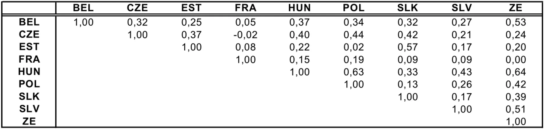
Table 8: Correlation of output business cycles on the period 1994:01-2004 :04
Note : Author Calculations
Table 9: Correlation of output business cycles on the period 1999:01-2004 :04
Note : Author Calculations
B E L C Z E E S T F R A H U N P O L S L K S L V Z E B E L 1,0 0 0 ,10 0,2 4 0 ,02 0,2 9 -0 ,0 9 0,2 2 0 ,2 0 0,2 8 C Z E 1 ,00 0,4 8 0 ,07 0,3 2 0 ,52 0,4 6 0 ,1 4 0,2 4 E S T 1,0 0 0 ,09 0,1 9 0 ,24 0,4 8 0 ,1 6 0,2 3 F R A 1 ,00 0,1 4 0 ,11 0,1 3 0 ,0 6 0,0 7 H U N 1,0 0 0 ,29 0,3 4 0 ,4 2 0,3 7 P O L 1 ,00 0,0 1 0 ,1 0 0,2 8 S L K 1,0 0 0 ,2 1 0,2 4 S L V 1 ,0 0 0,4 1 Z E 1,0 0
BEL CZE EST FRA HUN POL SLK SLV ZE
BEL 1,00 0,32 0,25 0,05 0,37 0,34 0,32 0,27 0,53 CZE 1,00 0,37 -0,02 0,40 0,44 0,42 0,21 0,24 EST 1,00 0,08 0,22 0,02 0,57 0,17 0,20 FRA 1,00 0,15 0,19 0,09 0,09 0,00 HUN 1,00 0,63 0,33 0,43 0,64 POL 1,00 0,13 0,26 0,42 SLK 1,00 0,17 0,39 SLV 1,00 0,51 ZE 1,00
Table 10: Correlation of output business cycles on the period 1994:01-1998 :12
Note : Author Calculations
Table 11: Correlation of output business cycles on the period 1994:01-2004:04
Note : Author Calculations
BEL C ZE EST FR A H U N LET L IT P O L S LK S L V Z E
BEL 1,00 0,21 0,37 0,64 0,45 0,26 0,41 0,61 0,18 0,39 0,69 C ZE 1,00 0,46 0,07 0,59 0,35 0,21 0,37 -0,24 0,30 0,17 EST 1,00 0,42 0,45 -0,15 0,80 0,29 -0,32 0,66 0,66 FR A 1,00 0,27 0,20 0,49 0,39 0,12 0,40 0,68 H U N 1,00 0,37 0,26 0,71 0,17 0,30 0,45 LET 1,00 -0,11 0,28 0,16 -0,07 0,10 LIT 1,00 0,23 -0,10 0,45 0,60 PO L 1,00 0,40 0,45 0,53 S LK 1,00 -0,12 0,04 SLV 1,00 0,64 ZE 1,00
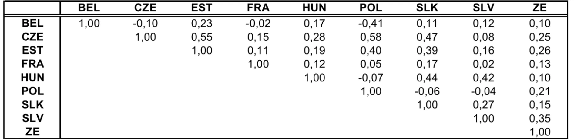
BEL CZE EST FRA HUN POL SLK SLV ZE
BEL 1,00 -0,10 0,23 -0,02 0,17 -0,41 0,11 0,12 0,10 CZE 1,00 0,55 0,15 0,28 0,58 0,47 0,08 0,25 EST 1,00 0,11 0,19 0,40 0,39 0,16 0,26 FRA 1,00 0,12 0,05 0,17 0,02 0,13 HUN 1,00 -0,07 0,44 0,42 0,10 POL 1,00 -0,06 -0,04 0,21 SLK 1,00 0,27 0,15 SLV 1,00 0,35 ZE 1,00
Table 12: Correlation of output business cycles on the period 1999:01-2004 :04
Note : Author Calculations
Table 13 : Correlation of output business cycles on the period 1994 :01-1998 :12
Note : Author Calculations
BEL CZE EST FRA HUN LET LIT P O L S LK SLV ZE
BEL 1,00 0,58 0,48 0,73 0,50 0,32 0,55 0,65 0,18 0,42 0,67 CZE 1,00 0,67 0,23 0,75 0,43 0,69 0,50 -0,08 0,25 0,50 EST 1,00 0,26 0,46 -0,14 0,66 0,31 -0,44 0,70 0,73 FRA 1,00 0,19 0,24 0,29 0,35 0,13 0,29 0,62 HUN 1,00 0,37 0,35 0,70 0,23 0,19 0,47 LET 1,00 0,33 0,26 0,49 -0,27 0,10 LIT 1,00 0,32 -0,20 0,52 0,57 PO L 1,00 0,45 0,41 0,55 S LK 1,00 -0,13 0,01 SLV 1,00 0,70 ZE 1,00
BEL C ZE EST FR A H U N LET L IT P O L S LK S L V Z E
BEL 1,00 -0,28 -0,02 0,31 0,15 0,12 0,19 0,43 0,50 0,16 0,69 C ZE 1,00 0,23 -0,29 0,51 0,26 -0,21 0,26 -0,57 0,40 -0,45 EST 1,00 0,35 0,34 -0,51 0,80 0,14 0,33 0,67 0,29 FR A 1,00 0,30 0,00 0,49 0,43 0,61 0,62 0,67 H U N 1,00 0,38 -0,08 0,73 0,19 0,70 0,16 LET 1,00 -0,71 0,37 -0,30 0,12 -0,10 LIT 1,00 -0,01 0,53 0,40 0,51 PO L 1,00 0,44 0,56 0,41 S LK 1,00 0,25 0,74 SLV 1,00 0,27 ZE 1,00
Appendix 2. The co-movements computed with un-conditional variance
The co-movements computed using the un-conditional variance has the following form:
VP (1 - Φ2)
VP*ij= (1)
(1 + Φ2) (1 - Φ2 – Φ1 ) (1 - Φ2 + Φ1)
Where VP = var(εtij), VP*ij = var(xt) and xt = ln Pit/Pjt.
Let’s demonstrate this relation. We consider the following equation: Xt - f1Xt-1- f2Xt-2 = et Þ Xt = f1Xt-1+ f2Xt-2 + et |. Xt – τ
Þ Xt Xt – τ = f1Xt-1Xt – τ + f2Xt-2 Xt – τ + et Xt – τ
Þ γτ = E(Xt Xt – τ) = E(f1Xt-1Xt – τ) + E(f2Xt-2 Xt – τ) + E(et Xt – τ). (2) Þ γτ = E(Xt Xt – τ) =f1E(Xt-1Xt – τ) +f2E(Xt-2 Xt – τ) + E(et Xt – τ). (3)
For τ=0, the relation (3) became: γ0 =f1E(Xt-1Xt) +f2E(Xt-2 Xt) + E(et Xt).
Þ γ0 =f1 γ1 +f2 γ2 + σ2ε Þ σ2x =f1 γ1+f2 γ2 + σ2ε (4)
For τ=1, the relation (3) can be written as follows :
γ1 = E(Xt Xt-1)=f1E(Xt-1Xt-1) +f2E(Xt-2 Xt-1) + E(et Xt-1).
But, E(et Xt-1) = 0. Þ γ1 =f1 σ2x +f2 γ1 (5) Þ γ1 -f2 γ1 =f1 σ2xÞ γ1(1-f2) =f1 σ2x
Þ γ1 = (f1 σ2x)/(1-f2) (6) with 1-f2 ≠ 0Þ f2 ≠ 1.
For τ = 2, the relation (3) becomes:
Þ γ2 = E(Xt Xt-2)=f1E(Xt-1Xt-2) +f2E(Xt-2 Xt-2) + E(et Xt-2), avec E(et Xt-2) = 0,
Þ γ2 =f1 γ1 +f2 σ2x (7). If we replaced in (4) the value γ2 obtained in (7), we have that:
σ2
x =f1 γ1+f2 γ2 + σ2ε Þ σ2x =f1 γ1+f2 (f1 γ1 +f2 σ2x ) + σ2ε Þ
Þ σ2
Þ σ2 x (1-f22) =f1 γ1+f2f1 γ1 + σ2ε Þ σ2x (1-f22) = γ1(f1 +f2f1) + σ2ε Þ σ2 x (1-f22) = [f1 σ2x/(1-f2)] (f1 +f2f1) + σ2ε Þ σ2 x (1-f22) – [σ2xf21 (1 +f2 )]/(1-f2) = σ2ε Þ σ2 x(1-f22) – [f21 (1 +f2 )/(1-f2)]} = σ2ε , with 1-f2 ≠ 0Þ f2 ≠ 1.
Finally, we obtain the relation (8) that is, the relation (1) written in a different manner. σ2
ε (1-f2)
Þ σ2
x = (8)
(1 + Φ1) (1 - Φ2- Φ1) (1 - Φ2+Φ1)