Job satisfaction and co-worker wages: Status or signal?

HAL Id: halshs-00587878

https://halshs.archives-ouvertes.fr/halshs-00587878

Preprint submitted on 21 Apr 2011

HAL is a multi-disciplinary open access

archive for the deposit and dissemination of sci-entific research documents, whether they are pub-lished or not. The documents may come from teaching and research institutions in France or abroad, or from public or private research centers.

L’archive ouverte pluridisciplinaire HAL, est destinée au dépôt et à la diffusion de documents scientifiques de niveau recherche, publiés ou non, émanant des établissements d’enseignement et de recherche français ou étrangers, des laboratoires publics ou privés.

Job satisfaction and co-worker wages: Status or signal?

Andrew E. Clark, Nicolai Kristensen, Niels Westergård-Nielsen

To cite this version:

Andrew E. Clark, Nicolai Kristensen, Niels Westergård-Nielsen. Job satisfaction and co-worker wages: Status or signal?. 2007. �halshs-00587878�

WORKING PAPER N° 2007 - 23

Job satisfaction and co-worker wages:

Status or signal?

Andrew E. Clark Nicolai Kristensen Niels Westergård-Nielsen

JEL Codes: C23, C25, D84, J28, J31, J33

Keywords: Job satisfaction, co-workers, comparison income, wage expectations, tournaments.

P

ARIS-JOURDAN

S

CIENCES

E

CONOMIQUES

L

ABORATOIRE D

’E

CONOMIE

A

PPLIQUÉE

-

INRA

48,BD JOURDAN –E.N.S.–75014PARIS TÉL. :33(0)143136300 – FAX :33(0)143136310

Job Satisfaction and Co-worker Wages:

Status or Signal?

Andrew E. Clark*, Nicolai Kristensen**and Niels Westergård-Nielsen***

September 2007

Abstract

This paper uses matched employer-employee panel data to show that individual job satisfaction is higher when other workers in the same establishment are better-paid. This runs contrary to a large literature which has found evidence of income comparisons in subjective well-being. We argue that the difference hinges on the nature of the reference group. We here use co-workers. Their wages not only induce jealousy, but also provide a signal about the worker’s own future earnings. Our positive estimated coefficient on others’ wages shows that this positive future earnings signal outweighs any negative status effect. This phenomenon is stronger for men, and in the private sector.

Keywords: Job Satisfaction, Co-workers, Comparison Income, Wage Expectations,

Tournaments.

JEL codes: C23, C25, D84, J28, J31, J33.

* _{Corresponding Author. Andrew.Clark@ens.fr. Paris School of Economics, IZA, CCP and Aarhus School}

of Business, University of Aarhus; **_{Aarhus School of Business, University of Aarhus, CIM and CCP;} ***

Aarhus School of Business, University of Aarhus, IZA and CCP. We thank Tor Eriksson, Takao Kato, Andrew Oswald and seminar participants at Amsterdam, the DTI Conference “New Perspectives on Job Satisfaction and Subjective Well-Being at Work” (London), the 24th _{JMA (Fribourg), Lyon 2, Rennes II,}

the Tinbergen Institute Workshop “Economics of the Workplace” Rotterdam (especially our discussant Mirjam van Praag), and the 2006 SOLE meetings for useful comments.

1 Introduction

A significant amount of work in the burgeoning literature on subjective well-being has focused on the role of relative income in determining satisfaction or happiness. Some labour-market examples are Capelli and Sherer (1988), Pfeffer and Langton (1993), Clark and Oswald (1996), Law and Wong (1998), Bygren (2004), Ferrer-i-Carbonell (2005), and Brown et al. (2007), using survey data, and Shafir et al. (1997) in experimental work.2 This work has generally concluded that relative wages are important in determining workers’ job or pay satisfaction. One implication is that the simple neoclassical utility model, where utility depends only on the individual’s own income or consumption, should probably be extended to incorporate relative income or consumption terms.

In parallel, the literature on establishment wage policies has highlighted the potential importance of wage compression. One prominent example is the fair wage-effort hypothesis formulated by Akerlof and Yellen (1990), which largely corresponds to Adams' (1963) theory of equity, in which effort depends on the relationship between fair and actual wages. In this theory, higher wages for some groups of workers – perhaps because they are in short supply – will raise wages for all of the workers in the establishment through the demand for pay equity.

The link between worker well-being and the establishment wage distribution is important for human resource managers, whose choice of pay policy will take into account the impact of worker dissatisfaction on profits and worker turnover (for empirical evidence, see Patterson et al., 2004). More broadly, wage comparisons may have

important consequences for the functioning of the entire labor market, explaining women’s labor force participation (Neumark and Postlewaite, 1998), unionization (Farber and Saks, 1980), money illusion (Shafir et al., 1997), hysteresis in unemployment (Summers, 1988, and Bewley, 1998), and wage rigidity (Levine, 1993, and Campbell and Kamlani, 1997).

The above literature appeals to the general area of preference interactions, as termed by Manski (2000), where what others do, or what happens to them, directly affects my own utility. While evidence of such income interactions has been steadily accumulating for a number of years, a smaller number of recent papers have uncovered empirical results of the opposite sign, with some measure of individual well-being being positively correlated with reference group income: the more others earn, the happier I am. This finding has been interpreted as demonstrating Hirschman’s tunnel effect (Hirschman and Rothschild, 1973): while others’ good fortune might make me jealous, it may also provide information about my own future prospects. Manski (2000) calls these phenomena expectations interactions, where what happens to others allows me to update my information set. The associated empirical work refers to information effects or signals.

In this paper we provide some of the first evidence that information effects may be stronger than comparison effects (i.e. that signal outweighs status) in the context of developed Western economies. Individuals may therefore be better off as others earn more, and consequently may not object to some degree of income inequality. We emphasize that the key parameter on which the balance between status and signal rests is the strength of the correlation between current reference group income and my own

future earnings. At the peer group or geographical level, this correlation is arguably small. In the context of Luttmer (2005), it is not because my neighbor receives a wage raise that my own future income prospects may necessarily look any brighter.

The signal effect is arguably far greater within the same establishment. In this paper we thus appeal to employer-employee panel data, and model individual job satisfaction as a function of the earnings of all other workers within the same establishment. This unusually rich data set results from the matching of survey panel data (over the period 1994-2001) to administrative longitudinal records of employer-employee data.

We show that workers are indeed more satisfied when their co-workers are better-paid. The “Hirschmanian establishment” or signal interpretation is that others’ wages provide sufficient information about my own future prospects to outweigh any jealousy I might feel towards my colleagues. This Hirschman effect is stronger for men than for women, and in the private sector.

We provide some further structure to this result by considering the “high-paid” and “low-paid”, those whose wages are respectively above and below the establishment mean wage. The correlation between satisfaction and the establishment mean wage for the high-paid is very insignificant. However, the satisfaction of the low-paid is strongly positively correlated with the establishment mean wage, which is consistent with the latter playing more of an information role for those with relatively low wages. These two results together yield the perhaps unpleasant implication that raising salaries towards the top of the wage distribution can make everyone happier: because their own wage has risen for the high-paid and for information reasons for the less well-off.

These results are broadly supportive of Tournament theory (Lazear and Rosen, 1981), where (some of) my colleagues’ current wages reflect my opportunities in the establishment’s internal labor market.

This paper is organized as follows. Section 2 presents a simple model of status and signal effects from others’ wages. Section 3 then describes the data that we use, and Section 4 presents the main empirical results. Last, Section 5 concludes.

2

Status or Signal?

There has been substantial interest across most of social science in the notion of status or comparisons to others. The very broad idea here is of negative externalities emanating from the consumption or income of others within the reference group: the more others earn, the lower is my utility, ceteris paribus. Empirically, the majority of work in this area has appealed to either measures of individual behaviour (such as labour supply or consumption), or measures of subjective well-being. In this latter case, a variable such as life satisfaction is shown to be positively correlated with own income, but negatively correlated with reference group income.3 The negative correlation is consistent with the presence of income comparison terms in the utility function.

Personnel Economics has arguably not paid much attention to such income comparison effects. However, it has underlined the incentive role played by the income that certain others within the same establishment may receive. In particular, in the tournament model (Lazear and Rosen, 1981) employees within a given establishment are seen as contestants for promotion. Relative worker performance determines the winner,

3 _{Where the reference group might be the individual’s peer group (those who share the same}

characteristics), others in the same household, the spouse/partner, friends, neighbors, work colleagues, or the individual herself in the past.

who receives a fixed prize set in advance. The level of individual effort then increases with the wage difference between winning and losing the tournament. High wages at the top of the establishment’s hierarchy are incentives for workers at lower job levels.

These two literatures confront each other when we consider individuals within the same establishment. In this case, one viable reference group is workers. As such, co-workers’ wages may have two opposing effects on individual utility. The first is a comparison or status effect, whereby co-workers’ higher wages make me feel relatively deprived, and the second is a signal effect, where higher co-worker wages provide me with information about my own future income prospects.

To illustrate this tension, we develop a simple model encompassing both status and signal effects. Imagine a simple linear utility function for individual i at time t:

*

it it it

U = αw + βw (1)

Here wit denotes the individual’s own wage and denotes the level of reference group

earnings, which in our model is the within-establishment average wage. We imagine that α>0 and a standard comparison story would have β<0; the latter reflects the importance of others’ income in the individual utility function. For expositional purposes, assume that there are two time periods, 1 and 2. There is a probability p that, if you stay in the same job, you will earn the reference group (establishment average) wage next year, increased by θ%, say. Otherwise you will earn w2. In addition, there is a chance δ of the

match finishing. If it does, you earn an outside wage of

* it

w

i

w next period, with “outside”

reference group earnings of * i

w . Individuals are assumed to maximize the present

discounted value of expected utility. Setting the discount rate to zero, without loss of generality, we have:

* i1 i1 i1 U = αw + βw

(

*

)

(

*

)

i2 1 2 2 U = δ αw_i+βw_i + (1- )δ α_⎣⎡p(1+θ)w_i + −(1 p w) _i ⎤_⎦+βw_i* So that

(

)

(

)

(

)

(

)

2 * * * 1 1 1 2 2 1 * * 1 1 2 (1 ) (1 ) (1 ) (1 ) (1 ) (1 ) (1 ) (1 ) it i i i i i i i t i i i i i U w w w w p w p w w w p w w w p w α β δ α β δ α θ β * * 2 i w α β δ α θ δ α β δ α δ β = ⎡ ⎤ = + + + + − _⎣ + + − _⎦+ = + + − + + + + − − + −

∑

It is assumed that individuals take their future into account, so that their satisfaction response today includes information on how they expect their job to be in the future4 (otherwise the information element plays no role).

A standard regression in the field of income comparisons models job/life satisfaction at time t as a function of both and . The δ(.) term, the third above, represents the outside options (in terms of both income and reference group income) should the match come to an end. This can be considered to be picked up by demographic variables, or by the individual effect in panel analyses. Most empirical estimation does not control for the levels of future income and reference group income ( and ) that pertain when the individual does not accede to the current reference group wage (although we can argue that wi2 will be closely correlated with ).

1 i w * 1 i w 2 i w * 12 w 1 i w

The key implication of this model is that the coefficient on in the estimation of * it w * it it it

U = αw + βw , will not only represent the comparison part of the utility function, but also the information that the establishment average wage (or whatever the measure of

4 _{This interpretation is explicitly tested in the context of worker quitting by Lévy-Garboua et al. (2007). A}

second piece of supporting evidence is that promotion opportunities attract a positive estimated coefficient in job satisfaction regressions.

reference group income is) provides about the worker’s future prospects. In our model, instead of estimating β, we in fact obtain an estimate of

= + (1- ) p(1+ )β β% δ α θ (2) This estimated coefficient,β% , will be positive, setting θ equal to zero for simplicity, if

(1 ) p β δ α − > − . Proposition 1:

The signal effect is more likely to dominate the status effect, so that others’ wages are positively correlated with my own well-being, as:

1) the probability of acceding to the reference group (p) is higher; 2) the jealousy parameter (β) is lower;

3) the match destruction rate (δ) is lower; and

4) the marginal utility of own income (α) is higher.

The empirical literature on income comparisons has taken the estimated value of β in (1) as an indicator of the strength of status effects. However, the simple model above highlights that this interpretation fails when there is also a signal component; in this case there is no clean test of comparisons as the estimated coefficient on picks up two opposing phenomena. In general, any estimated value of

*

w

β% will be consistent with the presence of income comparisons in the utility function. From (2), the strength of the comparison term can only be estimated in three distinct cases:

(i) α = 0, so that a priori only others’ income matters in the utility function, with no role

(ii) p=0, so that there is no chance of acceding to the reference group job. It might be

argued that a geographical definition of a reference group in Western countries, as in Luttmer (2005) or Blanchflower and Oswald (2004), goes some way to meeting this condition – I am perhaps relatively unlikely to end up with my neighbor’s job. This would likely be a worse assumption in the case of Knight and Song (2006), where the reference group (others in the same rural Chinese village) is more homogeneous.

(iii) δ=1. All matches are destroyed, so that there is no chance of staying in the same job. This is unlikely in field data, but can easily be engineered in experimental tests of comparison income, such as McBride (2007).

Our empirical work uses matched employer-employee data and considers a reference group of other workers within the same establishment. We therefore expect a non-zero information effect from others’ wages, especially for those who have a greater chance of moving up the establishment’s wage ladder, and for those who expect to stay in the establishment longer. This kind of data provides a good setting in which to test for the relative strength of status and signal effects.

3

Empirical Approach and Data

3.1 The Data

This paper is based on data of unusual richness. Eight waves of survey data from the Danish sample of the European Community Household Panel (ECHP)5 have been merged with administrative records. The ECHP survey data, which constitute a panel

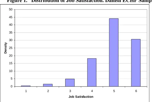
spanning 1994-2001, cover about 7,000 individuals in the first few years. Due to sample attrition this falls to about 5,000 individuals by 2001. Here we only consider employees, so that our effective sample size is reduced to about 16,000 observations on around 4,100 individuals over the whole eight-year period. Our dependent variable results from an overall job satisfaction question as follows:

How satisfied are you with your work or other main activity?

Respondents answer the satisfaction question using an ordered scale from 1 (not at all satisfied) to 6 (fully satisfied). Figure 1 shows the distribution of job satisfaction in this sample. As is usual, there is bunching towards the right-hand side of the satisfaction scale.

[Figure 1 about here]

The Danish component of the ECHP was sampled randomly from the central administrative database, the Central Personal Register (CPR). The CPR contains an entry for each individual in Denmark; each individual has a unique CPR number. This number can then be matched to the administrative IDA6 database, maintained by Statistics Denmark, containing labour market information on all individuals aged 15 to 74 (demographic characteristics, education, labor market experience, tenure and earnings) and employees in all workplaces in Denmark over the period 1980-2001. This database includes, amongst many other things, identifiers for both the firm and the establishment where the individual works, and the individual’s gross annual income. We therefore have administrative information on the income of all of the individual’s colleagues at their

place of work. Our use of administrative data likely reduces problems associated with measurement error regarding income.

By matching the two datasets we can thus obtain information on survey respondents' job satisfaction, their own wage, and the entire establishment wage distribution. In order for the concepts of relative wage and wage distribution to make sense, we limit the sample to establishments with a minimum of 5 colleagues.7 Our key regressions will model individual job satisfaction as a function of both own wages and a measure of others’ wages within the same establishment, as well as a set of standard demographic control variables.8

3.2 Econometric

Specification

We are interested here in the determinants of overall job satisfaction, and in particular the role of the individuals’ position in the establishment’s wage distribution. Job satisfaction is an ordered variable, reported on a scale from 1 to 6. In comparison to previous work that has considered the role of the establishment’s wage structure, our use of panel data means that we are able to control for unobserved individual characteristics. Lykken and Tellegen (1996) estimate that between 50% and 80% of the variation in individuals’ reported well-being results from genes and upbringing, underlining the importance of controlling for individual-specific fixed effects. However, introducing fixed effects in this particular case is problematic since the establishment’s average wage changes only little over time (and relatively few individuals change establishments), producing too little variation in the data to identify accurately the impact of reference

7 _{Using thresholds of 4 and 6 colleagues makes little difference to the results.}

group wages. In addition, individual random effects are likely to be inconsistent, as own wage is very likely endogenous in a model with job satisfaction as the dependent variable. As an ‘intermediate’ solution we therefore introduce a Mundlak correction term, as described below.

We assume a latent unobserved continuous measure of reported job satisfaction, , which is assumed to be a function of individual covariates such as age, education and other background characteristics,

*

JS

it

X and income-related terms,IT (which will also _it

be discussed below). The empirical model is then:

* _{' '}

it it it i it

JS =α IT +β X + +γ ε , i=1,...,N; t=1,...,Ti.

The error term is denoted byη_it = + , where γ ε_{i it} γ_i is the individual-specific time-invariant random component and ε_it is the individual and time-varying idiosyncratic disturbance term. Following the discussion above, we parameterize the individual effect

as '

0 1

i wi

γ =γ +γ , where w_i denotes the mean wage of individual i over all the waves in which she is observed. This term is included as an application of Mundlak’s (1978) method, where the individual effect is parameterized as a function of the mean values of some of the (time-varying) regressors that are thought to be correlated with the individual random effects. Wages are likely to be correlated with the individual random effect whereas, e.g., age is not a candidate since individuals grow older independently of personal traits.

The income-related terms,IT , consist of own wage, _it , and the average wage of all other employees at the same workplace, . To test for asymmetry in the way in

it

w

* it

which others’ wages affect job satisfaction, we follow Ferrer-i-Carbonell (2005) and define two variables, wage surplus and wage deficit, as follows:

i) If w_it > *, then wage surplus = ln( ) – ln( ) and wage deficit = 0.

it

w w_it *

it

w

ii) If w_it < *, then wage deficit = ln ( ) – ln( ) and wage surplus = 0.

it

w *

it

w w_it

iii) If w_it = *, then wage surplus = wage deficit = 0.9

it

w

Both wage surplus and wage deficit are thus weakly positive. If there is no asymmetry in

the effect of others’ wages, we expect the estimated coefficients on wage surplus and wage deficit to be equal and opposite in sign.

4 Results

In this section we first present the main results, and then a number of extensions. Finally, we discuss the results and their implications.

4.1 Basic

Results

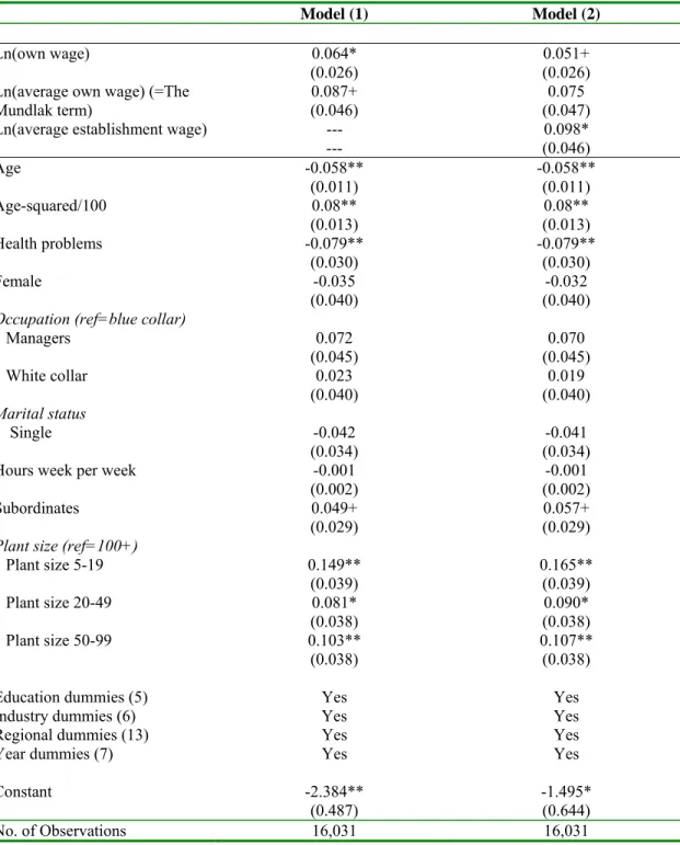
The first set of results, in Table 1, refers to the baseline model specification including the individuals’ own wage and the establishment average wage, as well as a number of other covariates. The key estimated parameters in these regressions refer to own wage and to the wage of the reference group (the establishment average wage).

[Table 1 about here]

9 _{Note that the specification of wage surplus and wage deficit actually yields the value function from}

There are two columns in Table 1. The first refers to a model without reference group information, but including both own income and the Mundlak income term; the second column adds the establishment average wage. The estimated coefficient on own income is positive and significant in both of these columns (at the five per cent level in column 1, and just outside that level in column 2). The estimated coefficient on the Mundlak term is positive in both columns, but only significant in column 1. The broad positive relationship between own income and job satisfaction, conditional on the other right-hand side variables, is unsurprising, and is consistent with most results in the literature.

More unusually, the estimated coefficient on the establishment average wage in column 2 is positive and significant at the 5 per cent level.10 In terms of our model, the signal effect thus dominates the status effect, yielding a net positive estimated coefficient. We therefore conclude that something akin to Hirschman’s tunnel effect appears to exist in these data. We discuss the implications of this finding in section 4.3 below.

The results for the other control variables are standard. We find a U-shape between job satisfaction and age (Clark et al., 1996), which minimizes here at age 36. We

also find a strong effect of health (although we cannot say anything about causality), and that employees in relatively small establishments (fewer than 100 employees) report statistically significant higher job satisfaction levels than do employees in establishments with 100 employees or more.

10_{In terms of the model in Section 2 we therefore have}

(1 ) p β δ α − > − .

We are interested in identifying certain groups for whom the signal effect of others’ wages may be stronger. To this end, we replace the establishment average wage used in Table 1 with the wage surplus and wage deficit variables defined in Section 3

above, both for the whole sample and by gender. These two new variables allow others’ wages to have asymmetric effects on job satisfaction, with a kink at = . We might in particular wonder whether the signal effect is stronger for those who earn less than the mean wage in the establishment. This asymmetry turns out to be important in explaining job satisfaction. The results for the whole sample, and separately by gender, are shown in Table 2.

it

w *

it

w

[Table 2 about here]

The parameter estimate on wage surplus is insignificant in all of these

regressions: the establishment average wage does not affect the job satisfaction of those who earn more than the mean wage in the establishment. On the contrary, over the whole sample the estimated coefficient on wage deficit is positive and significant at the 1 per

cent level (in Table 2): those who earn less than the establishment mean wage are more satisfied when they work in high-wage establishments. It is worth emphasizing that this correlation holds controlling for the individual’s own wage, so that the establishment wage is not acting as a proxy for own wages in these regressions.

This asymmetric effect of co-workers’ wages, depending on whether the individual earns more or less than the establishment average wage, is of interest for a number of reasons. In the first instance, it allows us to at least partially discount the

hypothesis that high-wage establishments are in some general sense pleasant places to work (for non-wage reasons): they could provide better non-monetary rewards or larger offices, for example. This explanation can only hold if any such benefits are specifically targeted towards lower-paid rather than higher-paid workers (which seems unlikely).

Dividing the sample by gender in Table 2, wage deficit remains positive and

highly significant for males, but is insignificant for women. This result might be thought of as a large-sample survey data counterpart to the well-known findings in the experimental literature that men react more strongly in competitive environments (Gneezy et al., 2003, and Niederle and Vesterlund, 2007).

4.2 Extensions

Tables 1 and 2 have shown that, at a given level of own wage, workers seem more satisfied in high-wage establishments. Our interpretation is that the signal effect of others’ wages (in terms of what I myself might hope to earn in the future) outweighs any status effect from wage comparisons. This sub-section presents a number of extensions to these basic results. The first two refer to different specifications of the establishment wage, while the last draws some links to tournament theory by showing that the signal effect from others’ wages is stronger for certain groups in the labor market.

Comparison to the 75th _percentile

The first issue we address is whether the linear-in-means specification is the most appropriate in the context of tournaments. In particular, this latter would suggest that only the wages of those above you in the hierarchy matter; as such the establishment average

wage may not be a particularly good measure. We thus replace the average establishment wage in the baseline specification by the 75th percentile wage. The results in the first column of Table 3 show that, again, workers are more satisfied in high-wage firms. The coefficient on the 75th percentile of the establishment wage is positive and significant.

[Table 3 about here]

We also suspect, in line with tournament theory, that the signal effect here will only apply to those who earn less than the 75th percentile wage, and that the size of this signal will increase the closer the individual is to the 75th percentile (from below). The last three columns of Table 3 explore this possibility, by running separate estimations according to whether the individual is in the bottom half of the wage distribution, the third quartile (i.e. the 50th to the 75th percentile) or the top quartile. The results accord with our prior: the effect of the 75th percentile wage is positive and significant for those in the first three quartiles, and especially for those in the third quartile (i.e. those who are closest to the establishment wage measure). By way of contrast, the 75th _{percentile wage}

is very insignificant for those in the top quartile of the establishment wage distribution.11

Additional Wage Comparisons by Occupation

A second specification issue refers to the sample used to calculate the establishment average wage. Up until now, we have used all workers in the

11 _{We can produce the same flavor of results with the 90}th _{percentile of the establishment wage. In this case}

the size of what we call the signal effect increases monotonically up to the 90th _{percentile, with the largest}

effect being found for workers between the 75th _{and the 90}th _{percentile; the effect for those in the top decile}

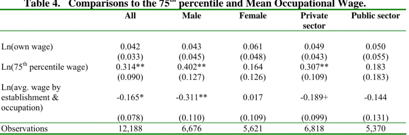
establishment. One topic of discussion in the income comparisons literature has been to whom individuals actually compare. Within the establishment, it is perhaps likely that workers compare their wages more to those of others who are doing the same kind of job. With this in mind, Table 4 shows the results of estimations with two establishment wage terms. The first is the 75th percentile establishment wage, as in Table 3: we expect this to reflect the signal component of others’ wages. The second is the mean wage by occupation, split up into three categories (Managers and equivalent, Middle-ranking positions, and Lower-level jobs).12 We calculate the 75th percentile establishment wage at the establishment level (and not by occupation within the establishment) as the whole ethos of tournaments is that the winners climb up the establishment hierarchy.

[Table 4 about here]

The results in the first column of Table 4 show the estimation results over the whole sample. These reveal a positive effect from the 75th percentile establishment wage, as before, but a negative significant effect from mean wage by occupation (within the establishment). We interpret the first of these as a signal effect, but the second as reflecting wage comparisons to similar others, as emphasized in much of the existing empirical literature.

Comparisons Differ between Labor Market Groups

The first column of Table 4 is consistent with the presence of both signal and status effects from others’ wages. The remaining columns of this table show that these

effects are not homogeneous across different labor market groups; in particular, both are stronger for men than for women and for private-sector workers than for public-sector workers.

Columns 2 and 3 of Table 4 show that, as already suggested in Table 2, signal effects from establishment wages are stronger for men than for women. The results here also show that the putative status wage effect is very significant and negative for men, but totally insignificant for women.

Finally, columns 4 and 5 of Table 4 show that the signal vs. status distinction in others’ wages is much sharper in the private than in the public sector. This is perhaps unsurprising, as wages in the Danish public sector are determined by centralized collective bargaining, with relatively little scope for individual establishments to set up wage tournaments.

4.3 Discussion and Implications

The results presented above are consistent with the interpretation that some individuals are inherently “Hirschmanian” within the establishment, in the sense that the signal effect from others’ wages dominates any jealousy or status effect. Consistent with tournament theory, the signal effect is always insignificant for those who earn more than the indicator of establishment wage that we employ.

The finding of a positive well-being effect from others’ wages differs from those in the majority of the published literature. We think that the key distinction lies in the composition of the reference group. As previously noted, the fact that the Joneses living next door earn more than I do, as in Luttmer (2005), may only reveal little information

about my future pay prospects: the entire effect of the Joneses’ pay thus passes by a comparison or status effect, reducing relative income and job satisfaction. Things may well be very different when work colleagues serve as the comparison group. In this case a high reference wage serves as a signal regarding one’s own future pay check.

The published work that has found a positive well-being effect from others’ income, Senik (2004 and 2007) and Kingdon and Knight (2007), can also be interpreted in terms of signal effects. Senik (2004) uses Russian RLMS data to establish a positive correlation between life satisfaction and (geographical) reference group income, especially for younger workers. In general, Senik (2007) makes the point that most evidence of comparison or jealousy effects comes from stable Western countries. In Senik’s work, the reference group consists of other people who are similar to you. In a very unstable labor market, what happens to similar others today may well be thought of as providing a signal about your own future labor market outcomes. Kingdon and Knight (2007) use South African data to show that the average income of others in the local residential area is positively correlated with household utility (while average income by district or province is negatively correlated with well-being). Again, this can be interpreted as showing that individuals are more likely to end up with their close neighbor’s job than with their more distant neighbor’s job.

This paper has uncovered this kind of signal effect using a natural reference group (colleagues within the same establishment) in an OECD country. Denmark has one of the most equal income distributions in the world, as well as very high income and wage mobility by international standards (OECD, 1997). These two facts together with our results suggest that: i) even in a stable economic environment there can be substantial

income mobility, and in this context it is not surprising that signal effects exist even in the affluent Danish economy; and ii) perhaps Danish income re-distribution has gone too

far. This latter point is arguably supported by the fact that increasing the pay of well-paid employees increases everyone’s job satisfaction. In Table 2, the well-paid’s job satisfaction rises because their own pay has gone up, and the low-paid’s job satisfaction increases via the establishment’s average wage. The provocative implication is that greater wage inequality within an establishment (via higher pay for the well-paid) may represent a Pareto improvement. This anti wage-compression result corresponds to some earlier findings in economics and psychology underlining a positive relationship between income inequality and measures of subjective well-being (see Clark, 2003, and the references therein).

5 Conclusion

A common theme in the subjective well-being literature has been comparisons to others, whereby low income relative to a reference group reduces well-being. We argue that this correlation is conditional on reference group income being uninformative about the individual’s own future income prospects. In much of the existing literature, this condition is satisfied (it is not necessarily because my neighbors or my cohort receive a pay rise that my own future prospects look brighter). We here analyze a data set where this condition probably does not hold, using wage information on all other workers within the same establishment. We do so by matching Danish ECHP data to administrative records.

The results are unambiguous. Job satisfaction is positively correlated with own wages, but it is also positively correlated with the average wage of all other workers within the same establishment. This Hirschman effect is stronger for men than for women, and in the private sector relative to the public sector. These findings are arguably consistent with the signal effect dominating the status effect for the subgroups that are most likely to be promoted. We also find that the signal effect is larger for those who earn less than the establishment wage measure.

Although we have not presented any direct tests of tournament theory, our results are nonetheless consistent with this model. When my colleagues earn higher wages, I learn about my future opportunities within the establishment. In line with the Tournament model this effect is more pronounced for men (who are more likely to be promoted), and in the private sector (where wage-setting is more individualized). Our results corroborate the findings of one of the few empirical studies of Tournament theory, Eriksson (1999), who finds support for this theory using Danish data.

Taking these results at face value, workers may not oppose wage inequality – at least not in the context of the firm’s pay scale. Indeed, in the current data, higher wages for better-paid workers will improve everyone’s job satisfaction. There are however likely limits beyond which this result will no longer hold. Future research should attempt to identify more accurately the relationship between worker well-being, on the one hand, and both own and others’ wages on the other, while explicitly recognizing that my own current relative wage misfortune may contain the promise of a brighter future.

6 References

Adams, J.S. (1963). Toward an Understanding of Inequity. Journal of Abnormal and Social Psychology, LXVII: 422-436.

Akerlof, G. A. and Yellen, J. L. (1990). The Fair Wage-Effort Hypothesis and Unemployment. Quarterly Journal of Economics, 105 (2): 255-283.

Bewley, T.F. (1998). Why not cut pay? European Economic Review, 42: 459-490.

Blanchflower, D.G. and Oswald, A.J. (2004). Well-being over time in Britain and the USA. Journal of Public Economics, vol. 88, pp. 1359-1386.

Brown, G.D.A., Gardner, J. Oswald, A. and Qian, J. (2007). Does Wage Rank Affect Employees' Wellbeing? Industrial Relations, forthcoming.

Bygren, M. (2004). Pay reference standards and pay satisfaction: what do workers evaluate their pay against?. Social Science Research, 33: 206-224.

Campbell, C.M. III and Kamlani, K.S. (1997). The Reasons for Wage Rigidity: Evidence from a Survey of Establishments. Quarterly Journal of Economics,

CXII: 759-789.

Capelli, P. and Sherer, P.D. (1988). Satisfaction, Market Wages and Labor Relations: An Airline Study. Industrial Relations, 27 (1): 56-73.

Clark, A.E. (2003). Inequality-Aversion and Income Mobility: A Direct Test. DELTA, Discussion Paper 2003-11.

Clark, A.E., Frijters, P. and Shields, M., (2007). Relative Income, Happiness and Utility: An Explanation for the Easterlin Paradox and Other Puzzles. Journal of Economic Literature, forthcoming.

Clark, A.E. and Oswald, A.J. (1996). Satisfaction and Comparison Income. Journal of Public Economics, 61 (3): 359-381.

Clark, A.E., Oswald, A.J. and Warr, P.B. (1996). Is Job Satisfaction U-shaped in Age?.

Journal of Occupational and Organizational Psychology, 69, 57-81.

Eriksson, T. (1999). Executive Compensation and Tournament Theory: Empirical Tests on Danish Data. Journal of Labor Economics, 17 (2): 262-280.

Farber, H.S. and Saks, D.H. (1980). Why Workers Want Unions: The Role of Relative Wages and Job Characteristics. Journal of Political Economy, 88 (2): 349-369.

Ferrer-i-Carbonell, A. (2005). Income and Well-Being: An Empirical Analysis of the Comparison Income Effect. Journal of Public Economics, 89 (5-6): 997-1019.

Gneezy, U., Niederle, M. and Rustichini, A. (2003). Performance in Competitive Environments: Gender Differences. Quarterly Journal of Economics, 118 (3):

1049-1074.

Hirschman, A. and Rothschild, M. (1973). The Changing Tolerance for Income Inequality in the Course of Economic Development. Quarterly Journal of Economics, 87, 544-566.

Kahneman, D. and Tversky, A. (1979). Prospect Theory: An Analysis of Decision Under Risk. Econometrica, 47: 263-291.

Kingdon, G. and Knight, J. (2007). Community, comparisons and subjective well-being in a divided society. Journal of Economic Behaviour & Organisation, 64:

69-90.

Knight, J. and Song, L. (2006). Subjective well-being and its determinants in rural China. University of Nottingham, mimeo.

Law, K.S. and Wong, C.-S. (1998). Relative importance of referents on pay satisfaction: A review and test of a new policy-capturing approach. Journal of Occupational and Organizational Psychology. 71: 47-60.

Lazear, E. and Rosen, S. (1981). Rank-Order Tournaments as Optimum Labor Contracts. Journal of Political Economy 89 (October 1981): 841-864.

Levine, D.I. (1993). Fairness, Markets and Ability to Pay: Evidence from Compensation Executives. American Economic Review, 83 (5): 1241-1259.

Lévy-Garboua, L., Montmarquette, C. and Simonnet, V. (2007). Job Satisfaction and Quits. Labour Economics, 14: 251-268.

Luttmer, E. (2005). Neighbors as Negatives: Relative Earnings and Well-Being.

Quarterly Journal of Economics, 120, 963-1002.

Lykken, D. and Tellegen, A. (1996). Happiness is a stochastic phenomenon.

Psychological Science, vol. 7, pp. 186-189.

Manski, C. (2000). Economic Analysis of Social Interactions. Journal of Economic Perspectives, 14, 115-136.

McBride, M. (2007). Money, Happiness, and Aspirations: An Experimental Study. University of California-Irvine, Working Paper 060721.

Mundlak Y. (1978) On the pooling of time-series and cross-section data. Econometrica 46 (1), 69:85.

Neumark, D. and Postlewaite, A. (1998). Relative Income Concerns and the Rise in Married Women’s Employment. Journal of Public Economics, 70 (1), 157-183.

Niederle, M. and Vesterlund, L. (2007). Do Women Shy Away from Competition? Do Men Compete Too Much? Quarterly Journal of Economics, 122 (3),

1067-1101.

OECD (1997). Employment Outlook. Paris: OECD.

Patterson, M., Warr, P. and West, M. (2004). Organizational Climate and Company Productivity: The Role of Employee Affect and Employee Level. Journal of Occupational and Organizational Psychology, 77, 193-216.

Pfeffer, J. and Langton, N. (1993). The Effect of Wage Dispersion on Satisfaction, Productivity, and Working Collaboratively: Evidence from College and University Faculty. Administrative Science Quarterly, 38:382-407.

Senik, C. (2004). When Information Dominates Comparison: A Panel Data Analysis Using Russian Subjective Data. Journal of Public Economics, 88, 2099-2123.

Senik, C. (2007). Ambition and Jealousy. Income Interactions in the "Old Europe" versus the "New Europe" and the United States. Economica, forthcoming.

Shafir, E., Diamond, P. and Tversky, A. (1997). Money Illusion. Quarterly Journal of Economics, 112 (2): 341-374.

Summers, L. H. (1988). Relative Wages, Efficiency Wages, and Keynesian Unemployment. American Economic Review, Papers and Proceedings, 78:

A. Results from random effects ordered probit models

Table 1. Baseline Specification.

Model (1) Model (2)

Ln(own wage) 0.064* 0.051+

(0.026) (0.026)

Ln(average own wage) (=The

Mundlak term) (0.046) 0.087+ (0.047) 0.075 Ln(average establishment wage) --- 0.098*

--- (0.046) Age -0.058** -0.058** (0.011) (0.011) Age-squared/100 0.08** 0.08** (0.013) (0.013) Health problems -0.079** -0.079** (0.030) (0.030) Female -0.035 -0.032 (0.040) (0.040)

Occupation (ref=blue collar)

Managers 0.072 0.070 (0.045) (0.045) White collar 0.023 0.019 (0.040) (0.040) Marital status Single -0.042 -0.041 (0.034) (0.034)

Hours week per week -0.001 -0.001

(0.002) (0.002)

Subordinates 0.049+ 0.057+

(0.029) (0.029)

Plant size (ref=100+)

Plant size 5-19 0.149** 0.165** (0.039) (0.039) Plant size 20-49 0.081* 0.090* (0.038) (0.038) Plant size 50-99 0.103** 0.107** (0.038) (0.038)

Education dummies (5) Yes Yes

Industry dummies (6) Yes Yes

Regional dummies (13) Yes Yes

Year dummies (7) Yes Yes

Constant -2.384** -1.495*

(0.487) (0.644)

No. of Observations 16,031 16,031

Table 2. Asymmetric Comparisons: Wage Surplus and Wage Deficit.

All Males Females

Ln(own wage) 0.218** 0.247** 0.182* (0.053) (0.075) (0.076) Wage surplus 0.038 0.063 -0.050 (0.065) (0.087) (0.100) Wage deficit 0.211** 0.282** 0.122 (0.060) (0.086) (0.084) No. of Observations 16,031 8,594 7,437

Note: Standard errors in parentheses + significant at 10%, * significant at 5%; ** significant at 1%. Other controls as in Table 1.

Table 3. Comparisons to the 75th percentile.

All Below Avg. Above Avg. but below 75th pctile Above 75th pctile Ln(own wage) 0.043 0.023 -0.405 0.222 (0.026) (0.033) (0.263) (0.146) Ln(75th _{percentile wage) 0.138** 0.207** 0.750** 0.0003} (0.048) (0.076) (0.269) (0.114) Observations 16,031 5,918 4,686 4,962

Notes: Standard errors in parentheses, + significant at 10%; * significant at 5%; ** significant at 1%. Other controls as in Table 1. Sample restricted to establishments with 10 or more employees.

Table 4. Comparisons to the 75th percentile and Mean Occupational Wage.

All Male Female Private sector Public sector Ln(own wage) 0.042 0.043 0.061 0.049 0.050 (0.033) (0.045) (0.048) (0.043) (0.055) Ln(75th _{percentile wage) 0.314** 0.402** 0.164 0.307** 0.183} (0.090) (0.127) (0.126) (0.109) (0.183) Ln(avg. wage by establishment & occupation) -0.165* -0.311** 0.017 -0.189+ -0.144 (0.078) (0.110) (0.109) (0.099) (0.131) Observations 12,188 6,676 5,621 6,818 5,370

Notes: Standard errors in parentheses, + significant at 10%; * significant at 5%; ** significant at 1%. Sample restricted to establishments with 10 or more employees.

B. Descriptive Statistics

Table B1. Means and Standard Deviations of Key Variables

Variable Mean Std. Dev.

Real wage/1000 (1994 DKK) 227.49 109.10 Age 40.29 10.66 Female 0.46 0.50 Occupation Managers 0.19 0.39 White collar 0.17 0.38 Blue collar 0.43 0.50 Health problems 0.20 0.40 Single 0.23 0.42 Hours work/week 37.28 6.99 Subordinates (Yes=1) 0.31 0.46 Establishment size 5-19 0.21 0.41 20-49 0.19 0.39 50-99 0.18 0.38 100 or more 0.26 0.44 Education Primary/Secondary 0.21 0.40 High School 0.07 0.25 Vocational 0.39 0.49 College-short 0.06 0.23 College-long 0.20 0.40 University 0.08 0.26

Note: The PPP exchange rate between the Danish Kroner (DKK) and the US dollar was 8.66 in 1994.

Figure 1. Distribution of Job Satisfaction. Danish ECHP Sample, 1994-2001.

0 5 10 15 20 25 30 35 40 45 50 1 2 3 4 5 6 Job Satisfaction De n s it y

Note: The question reads: How satisfied are you with your work or other main activity? Respondents report their level of satisfaction on an ordered scale from 1 (not at all satisfied) to 6 (fully satisfied).