HAL Id: hal-03049287
https://hal.archives-ouvertes.fr/hal-03049287
Submitted on 10 Dec 2020
HAL is a multi-disciplinary open access
archive for the deposit and dissemination of
sci-entific research documents, whether they are
pub-lished or not. The documents may come from
teaching and research institutions in France or
abroad, or from public or private research centers.
L’archive ouverte pluridisciplinaire HAL, est
destinée au dépôt et à la diffusion de documents
scientifiques de niveau recherche, publiés ou non,
émanant des établissements d’enseignement et de
recherche français ou étrangers, des laboratoires
publics ou privés.
atmospheric ozone and OH – an optimistic scenario and
a possible mitigation strategy
Ø. Hodnebrog, T. Berntsen, O. Dessens, M. Gauss, V. Grewe, I. Isaksen, B.
Koffi, G. Myhre, D. Olivié, M. Prather, et al.
To cite this version:
Ø. Hodnebrog, T. Berntsen, O. Dessens, M. Gauss, V. Grewe, et al.. Future impact of non-land based
traffic emissions on atmospheric ozone and OH – an optimistic scenario and a possible mitigation
strategy. Atmospheric Chemistry and Physics, European Geosciences Union, 2011, 11 (21),
pp.11293-11317. �10.5194/ACP-11-11293-2011�. �hal-03049287�
K. Ødemark1
1Department of Geosciences, University of Oslo, Norway
2Centre for Atmospheric Science, Department of Chemistry, Cambridge, UK 3Norwegian Meteorological Institute, Oslo, Norway
4Deutsches Zentrum f¨ur Luft- und Raumfahrt, Institut f¨ur Physik der Atmosph¨are, Oberpfaffenhofen, Germany 5Laboratoire des Sciences du Climat et de l’Environment (LSCE-IPSL), Gif-sur-Yvette, France
6Center for International Climate and Environmental Research-Oslo (CICERO), Oslo, Norway
7Centre National de Recherches M´et´eorologiques GAME/CNRM (M´et´eo-France, CNRS), Toulouse, France 8Department of Earth System Science, University of California, Irvine, USA
9Royal Netherlands Meteorological Institute, KNMI, De Bilt, The Netherlands *now at: CICERO, Oslo, Norway
**now at: UCL Energy Institute, University College London, London, UK
***now at: Department of Geosciences, University of Oslo, Norway and CICERO, Oslo, Norway
Received: 20 April 2011 – Published in Atmos. Chem. Phys. Discuss.: 16 June 2011 Revised: 24 September 2011 – Accepted: 31 October 2011 – Published: 14 November 2011
Abstract. The impact of future emissions from aviation and
shipping on the atmospheric chemical composition has been estimated using an ensemble of six different atmospheric chemistry models. This study considers an optimistic emis-sion scenario (B1) taking into account e.g. rapid introduction of clean and resource-efficient technologies, and a mitigation option for the aircraft sector (B1 ACARE), assuming further technological improvements. Results from sensitivity simu-lations, where emissions from each of the transport sectors were reduced by 5 %, show that emissions from both aircraft and shipping will have a larger impact on atmospheric ozone and OH in near future (2025; B1) and for longer time hori-zons (2050; B1) compared to recent time (2000). However, the ozone and OH impact from aircraft can be reduced sub-stantially in 2050 if the technological improvements consid-ered in the B1 ACARE will be achieved.
Shipping emissions have the largest impact in the ma-rine boundary layer and their ozone contribution may ex-ceed 4 ppbv (when scaling the response of the 5 % emis-sion perturbation to 100 % by applying a factor 20) over
Correspondence to: Ø. Hodnebrog
(oivind.hodnebrog@geo.uio.no)
the North Atlantic Ocean in the future (2050; B1) dur-ing northern summer (July). In the zonal mean, ship-induced ozone relative to the background levels may exceed 12 % near the surface. Corresponding numbers for OH are 6.0 × 10⁵molecules cm−3and 30 %, respectively. This large impact on OH from shipping leads to a relative methane lifetime reduction of 3.92 (±0.48) % on the global average in 2050 B1 (ensemble mean CH4lifetime is 8.0 (±1.0) yr),
compared to 3.68 (±0.47) % in 2000.
Aircraft emissions have about 4 times higher ozone en-hancement efficiency (ozone molecules enhanced relative to NOx molecules emitted) than shipping emissions, and the
maximum impact is found in the UTLS region. Zonal mean aircraft-induced ozone could reach up to 5 ppbv at northern mid- and high latitudes during future summer (July 2050; B1), while the relative impact peaks during northern win-ter (January) with a contribution of 4.2 %. Although the aviation-induced impact on OH is lower than for shipping, it still causes a reduction in the relative methane lifetime of 1.68 (±0.38) % in 2050 B1. However, for B1 ACARE the perturbation is reduced to 1.17 (±0.28) %, which is lower than the year 2000 estimate of 1.30 (±0.30) %.
Based on the fully scaled perturbations we calculate net radiative forcings from the six models taking into account
ozone, methane (including stratospheric water vapour), and methane-induced ozone changes. For the B1 scenario, ship-ping leads to a net cooling with radiative forcings of −28.0 (±5.1) and −30.8 (±4.8) mW m−2in 2025 and 2050, respec-tively, due to the large impact on OH and, thereby, methane lifetime reductions. Corresponding values for the aviation sector shows a net warming effect with 3.8 (±6.1) and 1.9 (±6.3) mW m−2, respectively, but with a small net cooling of -0.6 (±4.6) mW m−2for B1 ACARE in 2050.
1 Introduction
Increasing population and economic turnover will lead to in-creasing transport demand notably for aviation (AIR) and maritime shipping (SHIP). This will outpace technological improvements and lead to increasing emissions of various air pollutants, affecting air quality and climate through a com-plex system of chemical reactions and aerosol interactions. From a climate perspective, the present (2000) impact on ra-diative forcing (RF) is positive for AIR and negative for SHIP (Fuglestvedt et al., 2008; Balkanski et al., 2010), mostly due to formation of contrail cirrus in the first and sulphate in the latter. A first estimate of aircraft-induced cloudiness based on a climate model study was just recently given (Burkhardt and Karcher, 2011), however, the magnitude of positive RF from contrail cirrus is under debate (Lee et al., 2010). Sub-stantial contributions also stem from the emissions of nitro-gen oxides (NOx), carbon monoxide (CO) and non-methane
hydrocarbons (NMHCs). These relatively short-lived gases change the oxidative state of the atmosphere and tend to give a positive radiative forcing through the increase in ozone (e.g. Ramanathan and Dickinson, 1979; Berntsen et al., 1997), while enhanced OH levels are known to reduce the life-time of methane (CH4)and thereby cause negative RF (e.g.
Crutzen, 1987; Shindell et al., 2005). Among the various transport sectors, previous studies have shown that the warm-ing effect is most efficient (relative to the number of NOx
molecules emitted) for AIR (e.g. Fuglestvedt et al., 2008) because changes in ozone have their largest impact on cli-mate when they occur in the UTLS (upper troposphere/lower stratosphere) region, due to the low temperatures found near the tropopause (Wang and Sze, 1980; Lacis et al., 1990; Hansen et al., 1997). On the other hand, the cooling effect caused by changes in methane lifetimes dominates the SHIP impact (e.g. Myhre et al., 2011) because of the large amounts of NOxemitted into the clean maritime boundary layer. Due
to the different effects on the atmospheric composition, it is important to study the AIR and SHIP sectors individually, es-pecially when it comes to initiating mitigation measures. An-other important aspect regarding non-land based traffic emis-sions, as opposed to land based traffic emisemis-sions, is the fact that the background conditions are usually relatively clean
and this is known to increase the enhancement efficiencies of ozone and OH (e.g. Hoor et al., 2009).
IPCC (1999) published an assessment of the impact of aviation on climate, which was later updated by Sausen et al. (2005), and recently by Lee et al. (2009). Several other studies have also investigated how aircraft NOx emissions
alter the chemical composition of the atmosphere (e.g. Hi-dalgo and Crutzen, 1977; Johnson et al., 1992; Brasseur et al., 1996; Schumann, 1997; Grewe et al., 1999, 2007; Schu-mann et al., 2000; Kraabøl et al., 2002; Stevenson et al., 2004; Gauss et al., 2006; Søvde et al., 2007). The studies dealing with impact from future subsonic aircraft NOx
emis-sions project an increase in aircraft-induced ozone in 2050 compared to the present day atmosphere, but the effect de-pends on the emission scenario used. Søvde et al. (2007) estimated a maximum zonal mean aircraft-induced ozone in-crease of about 10 ppbv in the UTLS region for 2050 (an-nual mean) (aircraft NOx emissions of 2.18 TgN yr−1). In
another study, Grewe et al. (1999) calculated 7 to 10 % in-creased ozone mixing ratios due to aviation for the same year and region, but for two different emission scenarios (aircraft NOxemissions of 2.15 and 3.42 TgN yr−1, respectively).
Among the studies on impacts from ship emissions (e.g. Lawrence and Crutzen, 1999; Corbett and Koehler, 2003; Endresen et al., 2003, 2007; Eyring et al., 2005, 2007; Dalsøren and Isaksen, 2006; Dalsøren et al., 2009, 2010), only one has made future projections with atmospheric chemistry models (Eyring et al., 2007). They estimate max-imum near-surface ozone contributions from shipping of 5– 6 ppbv (annual mean) in the North Atlantic for the year 2000, increasing to 8 ppbv in one of the 2030 scenarios (ship NOx
emissions of 3.10 and 5.95 TgN yr−1, respectively). In a
sec-ond 2030 scenario the ship emissions were assumed to sta-bilize at 2000 levels, but the higher background NOxlevels
caused a slight decrease in the ozone impact from shipping. The present study is performed within the EU project QUANTIFY (Quantifying the Climate Impact of Global and European Transport Systems), which was the first attempt of investigating the global scale impact on the atmospheric composition due to emissions from each of the transport sectors. Fuglestvedt et al. (2008) investigated the climate forcing from the transport sectors for year 2000, and later Skeie et al. (2009) estimated transport-induced RF for fu-ture scenarios. A multi-model study of the year 2000 impact of transport emissions on the atmospheric chemical compo-sition was performed by Hoor et al. (2009) using the pre-liminary QUANTIFY emissions. They found a maximum ozone increase from aircraft of 3.69 ppbv in the upper tro-posphere between 30 and 60◦N, and they also found that shipping emissions contributed the most to ozone perturba-tions in the lower troposphere with around 50 % of the total traffic induced perturbation. The RF results from Hoor et al. (2009) were recently updated by Myhre et al. (2011) who used the final version of the QUANTIFY emissions data to estimate the year 2000 impact. The future impacts of both the
∗B1 ACARE aircraft emissions.
emissions and climate changes on transport-induced ozone have so far only been studied by Koffi et al. (2010), using the climate-chemistry model LMDz-INCA (also used in this study). Cariolle et al. (2009) investigated the effect of includ-ing an aircraft plume parameterization in large-scale atmo-spheric models, and similarly the inclusion of a ship plume parameterization was studied by Huszar et al. (2010). Both studies suggested significant reductions in non-land based traffic-induced ozone when plume processes were taken into account. Main results obtained in QUANTIFY are summa-rized in Lee et al. (2010) (aviation), Eyring et al. (2010) (shipping), and Uherek et al. (2010) (land transport).
The objective of this study is to investigate how emissions from the non-land based traffic sectors (AIR and SHIP) im-pact atmospheric ozone, OH, and the resulting RF, if precur-sor emissions from all sectors show reductions due to envi-ronmental concerns leading to improved technology. The ef-fects of possible future high emission scenarios will be dealt with in a follow-up study, using the same set of atmospheric chemistry models. The scenarios selected for this purpose are the SRES (Special Report on Emission Scenarios) opti-mistic B1 and pessiopti-mistic A1B (Nakicenovic et al., 2000), respectively, whereas results from the first are presented in this study. As the B1 scenario is considered to be far more optimistic than the A1B scenario (both for transport and non-transport emissions), due to assumptions of e.g. rapid intro-duction of clean and resource-efficient technologies in the first, the combined results represent possible low or high de-velopments, respectively, of the transport-induced impact on the atmospheric chemical composition, taking into account uncertainties related to the evolution of e.g. economy and technology. More specifically, the B1 scenario is charac-terized by environmental concerns leading to improved NOx
technology and a relatively smooth transition to alternative energy systems, but without assumptions of climate policies (in accordance with the SRES terms of reference) (Naki-cenovic et al., 2000). We have also studied the effect of utilizing additional technological improvements to the air-craft through the B1 ACARE mitigation option (Owen et
al., 2010). The fuel efficiency improvements in B1 ACARE probably require the technology to be driven by concerns over climate change and is thus considered a mitigation sce-nario. In the following we describe the simulation setup and the emission scenarios (Sect. 2), before giving a short presen-tation of each of the models in the ensemble (Sect. 3). The impacts on ozone and OH are dealt with in Sects. 4 and 5, respectively, while global radiative forcing calculations are presented in Sect. 6. Finally, our conclusions are given in Sect. 7.
2 Emissions and simulation setup
Traffic emissions of the ozone precursors NOx, CO and
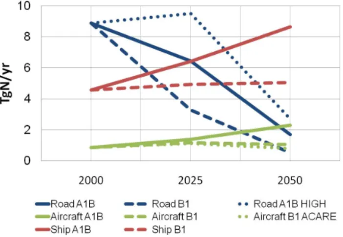
NMHC have been developed for year 2000 and for future scenarios through QUANTIFY (data can be downloaded from www.ip-quantify.eu). Anthropogenic emissions from non-traffic sources were taken from the EDGAR3.2-FT2000 inventory (Olivier et al., 2005; van Aardenne et al., 2005) for year 2000, while the future non-traffic emissions evolve according to the IPCC (Intergovernmental Panel on Climate Change) SRES (Nakicenovic et al., 2000) B1 scenario. Ta-ble 1 lists the global annual emissions used in this study, and Fig. 1 shows the time development of NOx emissions
from different transport sectors and for several scenarios. Al-though the future increase in the global NOxemissions from
AIR and SHIP is relatively small for the B1 scenario, impor-tant changes in the regional distribution of emissions can be seen for these transport sectors (Figs. 2–4).
New aircraft emissions scenarios have been developed us-ing the FAST model and are described in Owen et al. (2010). B1 ACARE is a mitigation scenario for aviation and con-tains additional emission reductions on top of the reductions that are assumed in the B1 scenario. B1 ACARE can be seen as a very optimistic, but feasible, scenario due to con-cern over climate change. The traffic demand is the same in both scenarios, but excellent fuel efficiency and NOx
im-provements are assumed in the mitigation scenario, in ac-cordance with the targets set by the Advisory Council for
Aeronautical Research in Europe (ACARE, 2002). Conse-quently, the B1 ACARE scenario has 4 and 24 % lower air-craft NOxemissions than B1 in 2025 and 2050, respectively,
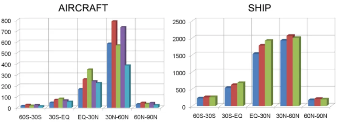
and the emissions for 2050 are even lower than the year 2000 estimate. Figure 2 shows that the increase in Europe and Asia in 2025 is smaller for B1 ACARE compared to the B1 sce-nario, and the emission reductions over the US are stronger in the first scenario. When comparing 2050 with 2025, only a few flight routes have increased emissions in B1 ACARE, and major emission reductions can be seen in Europe, the US, and Japan. The dependency of aircraft NOxemissions
on different latitude intervals can be seen in Fig. 4.
Shipping emissions are based on Endresen et al. (2007) (year 2000) and Eide et al. (2007) (years 2025 and 2050), and are characterized by increased NOxemissions in the
fu-ture, even for the optimistic B1 scenario. Already in 2025 the shipping sector could have become the largest emitter of NOx
among the three transport sectors (Fig. 1). Most of the in-crease for the B1 scenario is distributed among 12 new ship-ping routes (Fig. 3) that are predicted by Eide et al. (2007). It is worth noting the Northern Sea Route which has increasing emissions from 2000 to 2025, and then shows a slight decline from 2025 to 2050.
Emissions from road transport are based on Borken et al. (2007). Future emissions are documented in Uherek et al. (2010). While road traffic was the dominating source of NOxemissions among the transport sectors in 2000,
assump-tions of stricter vehicle emission standards and improve-ments in technology will lead to a substantial decrease of NOx emissions in the future scenarios (Fig. 1), particularly
for B1. Technology with low NOxemissions is already
avail-able for the road sector, and is faster to implement than for aircraft and shipping as the lifetime of vehicles is shorter. Koffi et al. (2010) showed that the rapid decline in NOx
emis-sions from road transport will lead to a drastic decrease in the ozone impact of road emissions in 2050. For this reason the impact of road traffic on ozone and OH has not been dealt with in this study, but model results from a policy failure sce-nario (A1B HIGH) for the road transport sector are subject of a follow-up study.
Additional emissions used in this study include biogenic emissions of isoprene and NO from soils (J¨ockel et al., 2006), lightning NOxemissions specified at 5 TgN yr−1(Schumann
and Huntrieser, 2007), and biomass burning emissions based on monthly mean Global Fire Emissions Database (GFED) estimates for 2000 (van der Werf et al., 2006) with multi-year (1997–2002) averaged activity data using emission fac-tors from Andreae and Merlet (2001). The biogenic and soil emissions are fixed using the climatology described in Hoor et al. (2009).
Regarding methane, all models used prescribed surface boundary conditions with global CH4 abundances taken
from IPCC (2001), but with a hemispheric scaling such that the mixing ratios were approximately 5 % higher in the Northern than the Southern Hemisphere. Two of the
Fig. 1. Time development of NOxemissions from different
trans-port sectors in the SRES A1B and B1 scenarios, together with the alternative scenarios B1 ACARE and A1B HIGH (unit: TgN yr−1).
models (p-TOMCAT and MOCAGE) used the IPCC (2001) value for 2000 (1760 ppbv) in all simulations, while the other four models (TM4, OsloCTM2, LMDz-INCA and UCI CTM) updated to the 2025B1 and 2050B1 values (1909 and 1881 ppbv, respectively) in the future simulations. The ef-fect of using 2000 rather than 2025B1 surface methane in the future 2025B1 simulations has been investigated with the OsloCTM2 model and found to have a small impact (up to 1–2 %) on aircraft- and ship-induced relative methane life-time changes, and on global distributions of ozone and OH perturbations.
The global models included in the ensemble have been run with year 2000 emissions and with the future emission sce-narios B1 and B1 ACARE for the years 2025 and 2050. For the year 2000 and for the future B1 simulations, a reference run (BASE) and perturbation runs, one for aircraft (AIR) and one for ship (SHIP), have been performed by each model for each year. For the future B1 ACARE simulations, new refer-ence runs and new aircraft perturbation runs were required in order to study the atmospheric chemistry impact of aircraft emissions under this scenario. In the perturbation simula-tions, a 5 % reduction has been applied to all emitted species of the respective traffic sector. The reasons not to switch off the emissions in the various transport sectors completely are both to reduce non-linearities in chemistry, and because the unscaled response (i.e. impacts due to 5 % emission pertur-bation) of the chemical system is expected to be closer to the effect of realistic emission changes than a total removal of the emissions (Hoor et al., 2009). The 5 % reduction approach was used to derive the sensitivity of the atmospheric chem-ical composition, e.g. ozone concentration, to an emission category with an appropriate accuracy (Hoor et al., 2009). The effect of, e.g. road traffic emissions is obtained by mul-tiplying this sensitivity, e.g. change in ozone concentration per kg emission from road traffic, with the total road traffic
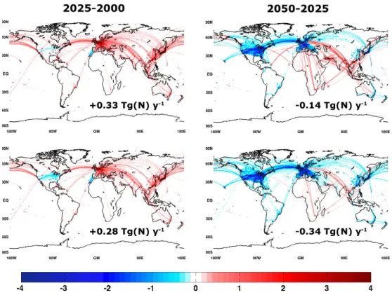
Fig. 2. Spatial distribution of the absolute difference in NOxemission flux from aircraft for the B1 (top) and B1 ACARE (bottom) scenarios
(unit: 10131molecules NO2m−2s−1)used in QUANTIFY.
Fig. 3. Spatial distribution of the absolute difference in NOxemission flux from shipping for the B1 scenario (unit: 10131molecules NO2
m−2s−1)used in QUANTIFY.
emissions. When comparing results from this study with other studies, it is important to note that the 5 % perturbation approach is very different from removing an emission source by 100 %. Non-linearities in chemistry can lead to large dif-ferences between the two approaches as described in Hoor et al. (2009) and Koffi et al. (2010). For further discussions on the small perturbation approach, the reader is referred to Grewe et al. (2010) who state that the method of perturbing an emission source by a small amount (e.g. 5 %), in order to
derive its sensitivity, is well suited to address impacts of e.g. future emission policies. In order to simplify the comparison with Hoor et al. (2009) and Myhre et al. (2011), the ozone and OH results (Sects. 4 and 5.1) are shown unscaled (i.e. the direct difference between BASE-AIR and BASE-SHIP), while calculations of methane lifetime changes and radiative forcings (Sects. 5.2 and 6) have been scaled to 100 % by mul-tiplying the impacts caused by the 5 % emission perturbation with 20 (i.e. 20 × (BASE-AIR) and 20 × (BASE-SHIP)).
Table 2. Specifications of the participating models in this study (modified from Hoor et al., 2009).
Model TM4 p-TOMCAT OsloCTM2 LMDz-INCA UCI CTM MOCAGE Operated KNMI UCAM-DCHEM UiO LSCE UCI M´et´eo-France Model type CTM CTM CTM CCM (nudged) CTM CTM Meteorology ECMWF OD ECMWF OD ECMWF OD ECMWF OD ECMWF OD ECMWF OD Hor. resolution 2◦×3◦ T21 T42 3.75◦×2.5◦ T42 T21
Levels 34 31 60 19 40 60
Model top (hPa) 0.1 10 0.1 3 2 0.1
Transport scheme Russell and Lerner (1981) Prather (1986) Prather (1986) van Leer (1977) Prather (1986) Williamson and Rasch (1989) Convection Tiedtke (1989) Tiedtke (1989) Tiedtke (1989) Emanuel (1991, 1993) Tiedtke (1989) Bechtold et al. (2001) Lightning Meijer et al. (2001) Price and Rind (1992) Price and Rind (1992) Price and Rind (1992), modified Price and Rind (1992) Climatology
Transp. species 26 35 76 66 28 65
Total species 42 51 98 96 38 82
Gas phase reactions 68+16 112+27 163+47 291+51 90+22 186+47
Het. Reactions 2 1 7 4 0 9
Strat. chemistry no no yes no LINOZ yes NMHC chemistry yes, CBM4 yes yes yes yes yes Lightning NOx(TgN yr−1) 5 5 5 2 5 5
References Williams et O’Connor et Gauss et al. (2003), Hauglustaine et al. (2004), Wild et al. (2003), Teyss`edre et al. (2010) al. (2005) Søvde et al. (2008) Folberth et al. (2006) Hsu et al. (2005) al. (2007)
3 Model descriptions
An ensemble of six models has been applied in order to estimate the future impact of non-land based traffic emis-sions on atmospheric ozone and OH, when considering op-timistic scenarios. For the results presented in Sects. 4– 6, equally weighted average values of the six models are shown along with the standard deviations, representing the spread in the model results (selected individual model results are shown in Appendix B). Five global Chemistry Trans-port Models (CTMs) were driven by operational meteoro-logical data from the European Centre for Medium-Range Weather Forecasts (ECMWF) and updated every 6 h (TM4, p-TOMCAT, OsloCTM2, UCI CTM and MOCAGE), while one Climate Chemistry Model (CCM) was nudged towards the ECMWF data (LMDz-INCA). In all simulations the me-teorological data are from year 2003 while 2002 data were used to spin-up the models. General model properties are synthesized in Table 2, and short descriptions are given be-low.
The models have been evaluated by Schnadt et al. (2010) who compared simulated CO to aircraft measurements from 2003, and found underestimation of tropospheric CO at northern hemispheric middle and subtropical latitudes. The discrepancies were possibly related to the biomass burn-ing emissions which were abnormally high in 2003 (e.g. Yurganov et al., 2005), while biomass burning emissions from 2000 were used in the simulations. Comparisons of the annual cycle of ozone from multi-year sonde observations and from the six models are shown in Appendix A (Fig. A1). Overall, the ensemble mean of the model results agrees rela-tively well with the observations.
3.1 TM4
TM4 is a global chemistry transport model with a horizon-tal resolution of 3◦×2◦and 34 vertical layers up to 0.1 hPa. The version used here has been comprehensively described in
Williams et al. (2010). The chemical scheme is the modified CBM4 mechanism decribed by Houweling et al. (1998), sup-plemented with sulphur chemistry and with the chemical re-action data being updated by Williams and van Noije (2008). The advection scheme is the slopes method developed by Russell and Lerner (1981), while convection is based on the Tiedtke mass flux scheme (Tiedtke, 1989).
3.2 p-TOMCAT
The global offline chemistry transport model p-TOMCAT is an updated version (see O’Connor et al., 2005) of a model previously used for a range of tropospheric chemistry stud-ies (Law et al., 1998, 2000; Savage et al., 2004). The model is used here with a horizontal resolution of 5.6◦×5.6◦
(T21) and extends from the surface to 10 hPa in 31 vertical levels. The chemical mechanism includes the reactions of methane, ethane and propane plus their oxidation products and of sulphur species. The model chemistry uses the atmo-spheric chemistry integration package ASAD (Carver et al., 1997) and is integrated with the IMPACT scheme of Carver and Stott (2000). The chemical rate coefficients used by p-TOMCAT are taken from the IUPAC summary of March 2005. The Prather (1986) scheme is used for advection while convective transport is based on the mass flux parameteriza-tion of Tiedtke (1989).
3.3 OsloCTM2
The OsloCTM2 chemistry transport model is used here with both tropospheric and stratospheric chemistry (Gauss et al., 2003; Søvde et al., 2008). It extends from the surface to 0.1 hPa in 60 vertical layers and a horizontal resolution of Gaussian T42 (2.8◦×2.8◦) is used. Advection in OsloCTM2 is done using the second order moment scheme (Prather, 1986), while convection is based on the Tiedtke mass flux scheme (Tiedtke, 1989). The Quasi Steady-State Approx-imation (Hesstvedt et al., 1978) is used for the numerical
Fig. 4. NOxemissions (Gg(N) yr−1)from aircraft (left) and shipping (right) for different latitude intervals and for different years/scenarios.
Note that 90◦S–60◦S is not shown in the figures because the emissions in this region are close to zero.
solution in the chemistry scheme, and photodissociation is done on-line using the FAST-J2 method (Wild et al., 2000; Bian and Prather, 2002).
3.4 LMDz-INCA
The LMDz-INCA model consists of the LMDz General Cir-culation Model (Le Treut et al., 1998), coupled on-line with the chemistry and aerosol model INCA (Folberth et al., 2006). The version 4.0 of the LMDz model has 19 hybrid levels on the vertical from the ground to 3 hPa and a horizon-tal resolution of 2.5◦in latitude and 3.75◦in longitude. The large-scale advection of tracers is performed using the finite volume transport scheme of Van Leer (1977), as described in Hourdin and Armengaud (1999). The turbulent mixing in the planetary boundary layer is based on a second-order closure model. The INCA model considers the surface and 3-D emissions, calculates dry deposition and wet scaveng-ing rates, and integrates in time the concentration of atmo-spheric species with a time step of 30 min. The CH4-NOx
-CO-O3 photochemistry, as well as the oxidation pathways
of non-methane hydrocarbons and non-methane volatile or-ganic compounds are taken into account. The winds and tem-perature predicted by LMDz have been nudged to 6-hourly ECMWF data over the whole model domain with a relax-ation time of 2.5 h (Hauglustaine et al., 2004).
3.5 UCI CTM
In this study, the University of California, Irvine (UCI) chem-istry transport model extends from the surface to 2 hPa with 40 vertical layers and is run at T42 horizontal resolution. The UCI CTM contains separate tropospheric and stratospheric chemistry. The tropospheric chemistry is simulated by the ASAD (A Self-contained Atmospheric chemistry coDe) soft-ware package (Carver et al., 1997) with UCI updates (Tang and Prather, 2010), which include the chemical kinetics and photochemical coefficients from the JPL publication 06–2
(Sander et al., 2006), and quasi steady-state initial guesses for radicals, and O(1D) included with O3. The stratospheric
chemistry uses the linearized ozone scheme (Linoz), which can include up to four independent species (e.g. O3, N2O,
NOy, CH4), but in this case consists only ozone (Prather and
Hsu, 2010). The tropopause, the boundary between the tro-posphere and the stratosphere, is determined by an artificial tracer (e90) (Prather et al., 2011; Tang et al., 2011). The ad-vection and conad-vection use the same schemes as OsloCTM2.
3.6 MOCAGE
The MOCAGE chemistry transport model is used here with a horizontal resolution of 5.6◦×5.6◦(T21) and 60 levels up to 0.1 hPa (Teyss`edre et al., 2007). The chemical scheme is a combination of the tropospheric RELACS scheme (Crassier et al., 2000) (a reduced version of the RACM scheme, Stockwell et al., 1997) and of the stratospheric REPROBUS scheme (Lef`evre et al., 1994) including the heterogeneous chemistry described in Luo et al. (1995). The large-scale transport of the tracers is done using a semi-Lagrangian transport scheme (Williamson and Rasch, 1989), while the convective transport is as described in Bechtold et al. (2001).
4 Ozone
The 2050 B1 annual mean ozone column response to a 5 % perturbation in emissions is shown in Fig. 5 for the aircraft and shipping sectors. The ozone impact from AIR is zonally well mixed, and mostly confined to the Northern Hemisphere (NH) in accordance with the latitudinal distribution of emis-sions shown in Fig. 4. A method to estimate the contribu-tion of a source is to estimate the sensitivity (ozone change per emission) with a 5 %-perturbation and then to multiply it with the total emission of the source category (e.g. AIR), which effectively equals a scaling of impacts to 100 % by multiplying the response of the 5 % emission perturbation by
Fig. 5. Yearly mean perturbations of the ozone column (1DU, up to 40 hPa) due to a 5 % perturbation of aircraft emissions (left) and ship
emissions (right) for the 2050 B1 scenario. The white contour lines show the standard deviation relative to the ensemble mean column perturbation (%), and have been smoothed to improve readability.
20 (Grewe et al., 2010). The results show a maximum ozone column response of 1.6 DU. The corresponding perturbation for SHIP is also 1.6 DU, but much less homogeneously dis-tributed with maximum values occurring over the North At-lantic Ocean and at the coastal areas of South East Asia. These two areas were also identified as peaks in the 2030 model simulations performed by Eyring et al. (2007), who attributed the increased ship-induced tropospheric ozone col-umn over the Indian Ocean to the higher tropopause and more effective vertical transport found there.
Figure 5 also shows the relative standard deviation which represents the spread in results between the different models (see Appendix B for individual model results). Only results for 2050 B1 are shown in Fig. 5, but the relative standard de-viations for the other years and scenarios also have similar distributions. The robustness of the models is quite good for the aircraft perturbation case, with a relative standard devi-ation less than 20 % in most of the areas where the pertur-bation effect is strong. However, model differences in inter-hemispheric transport result in a larger relative standard devi-ation in the Southern Hemisphere (SH). The relative standard deviation for shipping demonstrates larger deviations be-tween the models compared to the aircraft case, and is mainly in the range 30–40 %. One of the models (OsloCTM2) gives large impacts from shipping with a scaled maximum value of 2.5 DU, while another model (MOCAGE) has a correspond-ing value of only 0.9 DU. However, as model intercompari-son is beyond the scope of this study, the reader is referred to e.g. Danilin et al. (1998) and Rogers et al. (2002) for thor-ough discussions of differences between CTMs.
4.1 Effects of aircraft emissions
Figure 6 shows the impact of aircraft emissions on ozone in the UTLS region for January and July along with the differ-ence between the B1 and B1 ACARE scenarios (represented by the red lines). When focusing on the B1 scenario, the results indicate an increase in ozone impact from aircraft be-tween 2000 (black dotted line) and 2025 (black dashed line), while the difference between 2025 and 2050 (black solid
line) depends on the season and on the latitude. Because of the strong net decrease in NOxemissions from aircraft at
northern mid- and high latitudes from 2025 to 2050 (Fig. 4), the resulting ozone effect is a decrease in zonal mean values north of 30◦N during summer (Fig. 6, bottom right) when the photochemistry is more intense. This signal is to a large extent consistent between the models, but it depends strongly on the model whether or not there is an ozone decrease in the NH during winter. In the SH, the ozone impact from aircraft emissions is likely to increase in 2025 and further to 2050, if emissions evolve according to the B1 scenario. The zonal mean local maximum of 0.066 ppbv (or 1.3 ppbv scaled to 100 %) at about 25◦S in 2050 B1 (July) is caused by a com-bination of increased emissions in the tropics (Fig. 4) and transport across the hemispheres.
The local maximum can also be seen in Fig. 7, which shows the zonal mean ozone impact for 2050 B1 (see Fig. B1 for individual model results), together with the average verti-cal profile of the NH impact on ozone for each year and sce-nario. The results show that the maximum absolute impact in the UTLS region is larger in July compared to January, because of the difference in the length of the day between both months. However, the maximum ozone impact relative to the reference simulation (BASE) in 2050 B1 is larger in January with a peak value of 0.21 % (or 4.2 % scaled) lo-cated in the middle to upper troposphere at 20–30◦N. This peak in the tropics during winter arises because aircraft-induced NOxand O3are transported from the northern
mid-latitude UTLS to the low-mid-latitude middle troposphere where the background levels of NOxand O3are lower. For
compar-ison, Grewe et al. (1999) calculated annual maximum rela-tive ozone changes due to aircraft emissions of 7 % in a 2050 scenario, but the aircraft NOxemissions used in their study
were about twice as large as the 2050 B1 emissions that are used here (2.15 TgN yr−1compared to 1.05 TgN yr−1), and the surface NOxemissions were 60 % larger (69.7 TgN yr−1
compared to 43.8 TgN yr−1). The comparison is also influ-enced by several other factors such as the difference in year of meteorology used and potential model developments (e.g.
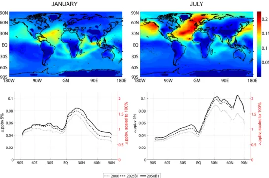
Fig. 6. Mean perturbations of ozone (1ppbv) in the upper troposphere (300–200 hPa) during January (left) and July (right) for the 2050
B1 scenario (top) and as zonal means for all scenarios (bottom). The color bar and the left y-axis show the unscaled impact of the 5 % perturbation of aircraft emissions (simulations BASE – AIR), while the red scales in the bottom figures are scaled up by a factor 20 from 5 % to 100 % and refer to all lines. The red lines show the difference between the B1 and B1ACARE scenarios and refer to the red axis only.
Fig. 7. Zonal mean perturbations of ozone (1ppbv) during January (left) and July (right) for the 2050 B1 scenario (top) and as Northern
Hemisphere average for all years (bottom). In the top figures, solid contour lines show the change relative to the BASE simulation while the dashed line indicates the tropopause. The color bar and the bottom x-axis show the unscaled impact of the 5 % perturbation of aircraft emissions (simulations BASE – AIR), while the red scales in the bottom figures are scaled up by a factor 20 from 5 % to 100 % and refer to all lines. The red lines show the difference between the B1 and B1ACARE scenarios and refer to the red axis only.
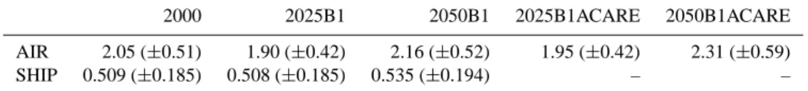
Table 3. Global annual average of the change in O3molecules per NOxmolecule emitted from aviation and shipping, given as ensemble
means and standard deviations.
2000 2025B1 2050B1 2025B1ACARE 2050B1ACARE
AIR 2.05 (±0.51) 1.90 (±0.42) 2.16 (±0.52) 1.95 (±0.42) 2.31 (±0.59) SHIP 0.509 (±0.185) 0.508 (±0.185) 0.535 (±0.194) – –
chemical reaction rates, deposition parameterizations, im-proved resolution) since the Grewe et al. (1999) study. Also worth noting is the fact that ozone perturbations in the lower troposphere are weaker during summer than in winter, pre-sumably because the surface deposition to plants is faster and the photochemical lifetime of ozone is shorter (because increased water vapour gives more HOxand thereby ozone
loss) at lower altitudes during summer.
If emissions evolve according to the B1 ACARE mitiga-tion opmitiga-tion rather than the B1 scenario, Figs. 6 and 7 show that ozone will only be reduced by a small amount in 2025 (red dashed line), while in 2050 (red solid line) the mitigation option will have a substantial effect on reducing ozone lev-els. A direct comparison between B1 and B1 ACARE yields mean ozone differences poleward of 30◦N in the UTLS of 0.18–0.30 ppbv and 0.94–1.40 ppbv during summers of 2025 and 2050, respectively (Fig. 6, red lines). Notably in the NH, the average ozone perturbation from aircraft in 2050 for B1 ACARE (blue solid line) is reduced to considerably lower values than the estimated impact in year 2000 (black dotted line) for altitudes below 200 hPa (Fig. 7). The fact that the mitigation option only has a minor effect in 2025 could be associated with the long lifetime of aircraft.
Hoor et al. (2009) found that the change in ozone bur-den per NOx-emission was highest for aircraft when
com-paring with the road and ship transport sectors. In Table 3 we have presented the ozone enhancement efficiency in or-der to investigate how the sensitivity changes with differ-ent years and scenarios. Previous studies (e.g. Grooß et al., 1998; Grewe et al., 1999) have found that the non-linearity in the ozone production normally leads to a smaller posi-tive ozone perturbation per aircraft emitted NOx-molecule
when the emissions are higher. This is also the case when we compare the ozone change per aircraft NOx-emission in
2000 with 2025 (Table 3), when the emissions are expected to increase. However, when looking at the 2050 B1 scenario, all models show a higher ozone enhancement efficiency com-pared to year 2000, although the aircraft NOxemissions also
are higher. This unexpected effect can be explained by the change in the location of the emissions. In 2050, the aircraft NOx emissions are shifted further south compared to year
2025 (Fig. 4), and will then take place in more pristine re-gions where the background NOxlevels are lower.
Addition-ally, Hoor et al. (2009) emphasized the role of road traffic for the chemical state of the UTLS, and as NOxemissions
from this transport sector are assumed to decrease rapidly in the future, the NOxbackground levels at cruise altitude are
affected. Not surprisingly, the highest ozone enhancement efficiency is found in 2050 B1 ACARE, which is the sce-nario with the lowest aircraft emissions. For this case, the models estimate that the ozone abundance increases by 2.31 molecules for every NOxmolecule emitted from aircraft. 4.2 Effects of ship emissions
Figures 8 and 9 show the effects of shipping emissions on atmospheric ozone in January and July for different years and scenarios (see Fig. B2 for individual model results). Even if emissions evolve according to the optimistic B1 sce-nario, model results show that the shipping sector will in-crease its effect on ozone in the future. Focusing on the es-timated ozone impact in the lower troposphere in 2050 B1 (Fig. 8), the largest effect from shipping can be found in the North Atlantic Ocean with ozone values of about 0.2 ppbv (or 4 ppbv scaled) during summer when the photochemical activity reaches a maximum. Notably, the impact in the Arc-tic region is expected to increase in the future due to the ex-pected introduction of new ship tracks associated with melt-ing of the polar ice cap. This area is especially sensitive to emission perturbations because of the low background NOx
levels which lead to higher ozone enhancement efficiencies. Consequently, the maximum relative effects in July are found in this region, showing zonal mean impacts exceeding 0.6 % (or 12 % scaled) near the surface (Fig. 9).
Interestingly, Fig. 8 shows that the ozone impact from shipping at northern mid- and high latitudes will increase from 2025 (dashed line) to 2050 (solid line), especially dur-ing winter, although the emissions in these regions are ex-pected to decrease (Fig. 4). Except for transport from lower latitudes, where the emissions increase, this feature can be explained by lower ambient levels of NOxwhich act to
in-crease the change in ozone burden per NOx emitted from
ships. The increase in ozone enhancement efficiency can also be seen in Table 3, where global annual average values are given. In the future B1 scenario, large reductions in anthro-pogenic non-traffic and road emissions of NOxare assumed
over the Eastern US and Europe. This significantly increases the ozone enhancement efficiency from shipping, as trans-port from these polluted continental areas normally leads to higher levels of NOxover the Atlantic Ocean and the North
Fig. 8. Mean perturbations of ozone (1ppbv) in the lower troposphere (>800 hPa) during January (left) and July (right) for the 2050 B1
scenario (top) and as zonal means for all years (bottom). The color bar and the left y-axis show the impact caused by a 5 % perturbation of ship emissions (simulations BASE – SHIP), while the red scales in the bottom figures are scaled up by a factor 20 from 5 % to 100 %.
Fig. 9. Zonal mean perturbations of ozone (1ppbv) during January (left) and July (right) for the 2050 B1 scenario (top) and as Northern
Hemisphere average for all years (bottom). In the top figures, solid contour lines show the change relative to the BASE simulation while the dashed line indicates the tropopause. The color bar and the bottom x-axis show the impact caused by a 5 % perturbation of ship emissions (simulations BASE – SHIP), while the red scales in the bottom figures are scaled up by a factor 20 from 5 % to 100 %.
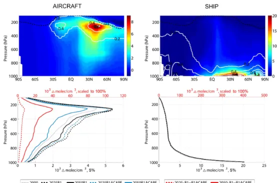
Fig. 10. Mean perturbations of OH (1031molec cm−3)in July in the upper troposphere (300–200 hPa) due to a 5 % perturbation of aircraft emissions (left), and in the lower troposphere (>800 hPa) due to a 5 % perturbation of ship emissions (right). The top row figures show results from the 2050 B1 scenario, and the bottom row figures show zonal means for all years and scenarios. The colorbars and the left y-axis show the unscaled impact of the 5 % perturbation of the emissions, while the red scales in the bottom figures are scaled up by a factor 20 from 5 % to 100 % and refer to all lines. The red lines show the difference between the B1 and B1ACARE scenarios and refer to the red axis only. Note that different scales are used for AIR and SHIP.
5 OH
5.1 Global OH
Changes in the concentration and distribution of the hydroxyl radical (OH) are important for air pollution and the self-cleaning capacity of the atmosphere (Lelieveld et al., 2002) as OH is the main oxidant in the troposphere. Validation of modelled OH is difficult, however, particularly because of its short lifetime (less than one second) which makes it almost impossible to measure directly. In a recent study by Montzka et al. (2011), indirect measurements of the interannual vari-ability of global OH are consistent with past model studies (Dentener et al., 2003; Dalsøren and Isaksen, 2006; Lelieveld et al., 2006; Duncan and Logan, 2008), and this suggest that larger confidence should be given to models than previously assumed (Isaksen and Dalsøren, 2011).
The impact of aircraft and shipping emissions on tropo-spheric OH is shown in Figs. 10 and 11 for July, when the effect is largest due to enhanced photochemistry in the NH. For aircraft emissions, there is an indication of a future in-crease in the impact on tropospheric OH. Figure 10 shows that enhanced OH levels in the UTLS are expected at all lat-itudes in 2025 (black and blue dashed lines), with an excep-tion near the Arctic region where increased aircraft emissions seem to cause a slight decrease in OH levels. However, when
comparing the impacts between 2025 and 2050, the OH re-sponse depends strongly on both scenario and latitude. In 2050 (black and blue solid lines), a decrease is seen between approximately 30 and 60◦N, associated with a strong de-crease in aircraft NOxemissions (Fig. 4), while a zonal mean
increase is expected elsewhere, in particular near the equa-tor where aircraft NOx emissions are assumed to increase.
In 2025 B1, the zonal mean average in the UTLS region for July peaks at 40◦N with a value of 8.6 × 10³molecules cm−3 (unscaled). When averaging the aircraft-induced OH verti-cal profile over the entire NH, 2025 B1 and 2050 B1 both show a maximum of 5.4 × 10³molecules cm−3 (unscaled) near 250 hPa (Fig. 11).
The largest effects from aircraft emissions during north-ern summer in the future (July 2050; B1) can be found east and southeast of Asia, but also with significant impacts close to the North Atlantic flight corridor (Fig. 10, top left). The zonal mean OH impact peaks above 300 hPa, and this is also the region of maximum relative impact with a value of 0.6 % (or 12 % scaled) (Fig. 11, top left). In the SH, the absolute values are lower, but due to low background levels the rel-ative impact is fairly high with a value of almost 0.5 % (or 10 % scaled).
As was the case with ozone, the technological improve-ments that are assumed in the B1 ACARE mitigation sce-nario have significant effects on OH. If the ACARE targets
Fig. 11. Zonal mean perturbations of OH (1031molec cm−3)in July due to a 5 % perturbation of aircraft emissions (left) and ship emissions (right), for the 2050 B1 scenario (top) and the average Northern Hemisphere vertical profile for all years and scenarios (bottom). In the top figures, solid contour lines show the change relative to the BASE simulation while the dashed line indicates the tropopause. The colorbar and the bottom x-axis show the unscaled impact of the 5 % perturbation of the emissions, while the red scales in the bottom figures are scaled up by a factor 20 from 5 % to 100 % and refer to all lines. The red lines show the difference between the B1 and B1ACARE scenarios and refer to the red axis only. Note that different scales are used for AIR and SHIP.
will be met in 2050, the northern summer OH levels in the UTLS region (red solid line) could be reduced by up to 5.7 × 10⁴molecules cm−3 (Fig. 10, bottom left). The reductions are substantial also in the NH as a whole, showing average differences between B1 and B1 ACARE of 3.9 × 10⁴molecules cm−3 near 250 hPa (Fig. 11, bot-tom left), and with significant effects also in the mid-dle troposphere. In the near future (2025), the gain of fulfilling the ACARE targets is much lower, but still the maximum difference between B1 and B1 ACARE is 7.6 × 10³molecules cm−3(red dashed line).
Hoor et al. (2009) emphasized the large impact of ship emissions on the boundary layer OH levels, and concluded that the effect of ship emissions is more important for the global OH budget than road and aircraft emissions. Fig-ure 10 shows that the impact from ship emissions on OH in the boundary layer is expected to increase in the future if emissions evolve according to the B1 scenario. Between 2025 and 2050, OH will continue to increase at all latitudes except north of 60◦N where a small reduction in ship NO
x
emissions is expected.
Focusing on northern summer in the future (July 2050; B1), the largest impact from ship emissions can be found in the North Atlantic Ocean with maximum values reach-ing 3.0 × 10⁴molecules cm−3(unscaled) (Fig. 10, top right).
As discussed in Sect. 4.2, ozone production in this area is largely sensitive to an increase in NOx emissions, and
be-cause of high humidity and strong incoming solar radiation, additional OH is produced when O(1D) reacts with H2O.
Ad-ditionally, the background levels of CO and NMHCs, which act to deplete OH, are relatively low in these pristine regions. In the zonal mean, maximum absolute values are found near the surface at 45◦N (Fig. 11, top right), while the relative
impact reaches a maximum of about 1.5 % (or 30 % scaled) near 75◦N. The reason is the low background values of OH,
as shipping is a dominant source of air pollutants at these high latitudes, and because the production of additional OH caused by ship emissions is more effective in the summer month of July.
5.2 Methane lifetime
Emissions from the aircraft and shipping sectors greatly af-fect the OH concentration, and this leads to changes in the methane lifetime. Methane lifetimes due to reaction with OH have been calculated for each model and for each year and scenario. As in Hoor et al. (2009), monthly mean 3-D-fields of methane and OH were used, and the resulting life-time changes were then scaled from a 5 % perturbation in emissions to a 100 % perturbation (to get a stronger signal in the RF calculations) by multiplying with a factor of 20
Table 4. Relative changes (%) in methane lifetimes (integrated up
to 50 hPa) due to a 5 % decrease in traffic emissions. Values are given relative to the BASE case, and are scaled to 100 % by multi-plying with 20. Both the mean of the six models and the standard deviations (indicating the spread of the models) are given. Note that this table does not include the feedback effect of methane changes on its own lifetime.
AIR SHIP 2000 1.30 (±0.30) 3.68 (±0.47) 2025B1 1.69 (±0.35) 3.73 (±0.40) 2050B1 1.68 (±0.38) 3.92 (±0.48) 2025B1ACARE 1.59 (±0.34) – 2050B1ACARE 1.17 (±0.28) –
(Grewe et al., 2010). The resulting model mean and standard deviation of the methane lifetime changes are given in Ta-ble 4 (see TaTa-bles B1–B2 for individual model results), while the model mean of the methane lifetime is 8.0 (±1.0) yr in the 2050 B1 BASE simulation and 8.3 (±1.0) yr in the 2000 BASE simulation. The rather low relative standard deviation of 12 % is similar for the BASE simulations of the other sce-narios, and indicates that the ensemble mean of the models is relatively robust when calculating methane lifetimes.
As discussed in Sect. 5.1, SHIP exhibits the largest impact on OH levels and consequently the largest impact on methane lifetime. The model ensemble predicts that the shipping sec-tor contributed to a methane lifetime reduction of 3.68 % in year 2000, and that this number will increase to 3.92 % in 2050, if emissions evolve according to the B1 scenario (Table 4). Eyring et al. (2007) calculated methane lifetime changes from shipping in 2030, and their estimates range from 1.14 % to 1.81 % for a low and high emission scenario, respectively. Their result is much lower than both 2025 B1 and 2050 B1 from this study, and that was also the case for the year 2000 results discussed in Hoor et al. (2009). Ac-cording to Hoor et al. (2009), part of the differences could be attributed to the very different distribution of ship emissions. The same reasoning applies here as the future ship emissions in Eyring et al. (2007) are more concentrated along the ma-jor shipping routes in contrast to the QUANTIFY future ship emissions, which are spread out over larger areas.
The methane lifetime changes for SHIP do not follow the trend in ship NOxemissions, which increased a lot more
be-tween 2000 and 2025 B1 than bebe-tween 2025 B1 and 2050 B1 (Fig. 1). The reason is the assumption of large reduc-tions in land based NOx emissions, particularly from road
traffic, in Europe and the US between 2025 B1 and 2050 B1 (not shown). This effect exceeds the impact of increased ship emissions, as a decrease in background NOxlevels leads to a
more efficient OH production from shipping.
The future methane lifetime changes for AIR are to a cer-tain degree in accordance with the evolution of the aircraft
B1 emissions; an increased impact in 2025 followed by sta-bilization in 2050 (Table 4). The model ensemble predicts a much lower impact of aircraft on methane lifetimes for the B1 ACARE scenario, especially in 2050 when the relative methane lifetime change is lower than the year 2000 value.
6 Radiative forcings
Radiative forcings have been calculated using the same method as in Myhre et al. (2011). The Oslo radiative transfer model (Myhre et al., 2000) was used to calculate ozone radia-tive forcings based on monthly mean ozone fields from each model simulation. In order to obtain a robust signal the fully scaled perturbations have been used in the RF calculations, i.e. the ozone change resulting from the 5 % perturbation has been multiplied by 20 (Hoor et al., 2009; Grewe et al., 2010). According to Myhre et al. (2011), the non-linearities aris-ing from the perturbation magnitude are of little importance compared to the inter-model differences in the RF.
Figure 12 shows the yearly averaged ozone RF for the 2050 B1 scenario as means of all models and with absolute standard deviations. The aircraft sector has a larger impact than ship emissions in the NH and the changes in RF are relatively homogeneous throughout different latitude zones. The impacts are large throughout the NH and have maximum values reaching 76 mW m−2near 30◦N. In the SH the ozone RF from aircraft is low, except in the region 0–30◦S. This latitude band also shows a large spread of the models with standard deviations up to 21 mW m−2, indicating possible model uncertainties related to convection and transport be-tween the hemispheres. For SHIP, the ozone RF is stronger in the SH compared to AIR, but the RF in the NH is much weaker. Maximum impact from SHIP takes place between 30◦N and 30◦S, and peaks at 50 mW m−2.
Global average ozone RF for all scenarios is given in Ta-ble 5 (see TaTa-bles B3–B4 for individual model results). For the B1 scenario there is a small increase in the ozone RF from AIR between 2025 and 2050, although the NOxemissions
from aircraft are assumed to decrease slightly during this time span. As explained in Sect. 4.1, this is probably caused by the latitudinal shift in the location of the aircraft emissions leading to higher ozone enhancement efficiencies in 2050. For comparison, Myhre et al. (2011) calculated a five model average of 17 mW m−2for AIR in year 2000. The increase to 25.7 mW m−2for 2025 B1 (Table 5) is consistent with the
aircraft NOxemissions, which also are assumed to increase
(Fig. 1). For the 2050 B1 scenario, Skeie et al. (2009) esti-mated ozone RF from AIR to be 38 mW m−2using a simple climate model. The relatively large difference to our study can be partly explained by a lower normalized radiative forc-ing in this study (36.3 compared to 42.9 mW m−2DU−1), and partly by lower ozone enhancement efficiencies (2.16 com-pared to 2.69 ozone molecules enhanced per NOxmolecule
Fig. 12. Radiative forcing (mW m−2)from short-term O3due to emissions from aircraft (left) and shipping (right), shown as ensemble mean
for the 2050 B1 scenario (top) along with the absolute standard deviation (bottom). Note that the fully scaled perturbations were used to calculate the forcings.
was used to estimate the aviation RF of ozone in 2050 to be in the range 59.4–109.8 mW m−2, depending on the sce-nario. Their estimates are much higher than in this study, but this is expected because even their lowest emission scenario (SRES B2 with technology 2, see IPCC, 1999) had larger aircraft NOxemissions than the 2050 B1 scenario used here.
The effect of the B1 ACARE mitigation strategy is evident already in 2025, with a 1.6 mW m−2 lower ozone RF than
in the B1 scenario (Table 5). However, in 2050 the corre-sponding number has increased to 7.3 mW m−2, showing the large potential impact of technological improvements in the aircraft sector.
The ozone RF from SHIP is calculated to increase be-tween 2025 and 2050, this time due to a combination of the slight increase in ozone precursor emissions for this trans-port sector, and the stronger ozone enhancement efficiency in 2050 (see Sect. 4.2). Despite the assumed increase in ship emissions between 2000 and 2025 B1, Myhre et al. (2011)
have a larger estimate for 2000 (24 mW m−2)than our re-sults for 2025 B1. The reason is that the MOCAGE model is included in our study, and this model is at the lower end of the spectrum when calculating ozone RF from SHIP (Ta-ble B4). Again, Eyring et al. (2007) calculated lower impacts than in this study, with ozone RF from shipping ranging from 7.9 to 13.6 mW m−2 in 2030. On the other hand, Skeie et
al. (2009) estimated a larger impact from shipping with short-lived ozone RF at 36 mW m−2for the 2050 B1 scenario, also this time due to lower ozone enhancement efficiencies in this study (0.535 compared to 0.859 ozone molecules enhanced per NOxmolecule emitted from SHIP).
Emissions of NOxfrom aircraft and shipping sectors
nor-mally lead to an increase in OH concentrations, resulting in a reduction of methane lifetime. The forcing due to the changes in methane is given in the second column in Table 5, and has been calculated mainly using the method described by Berntsen et al. (2005). For each year and scenario, the
changes in methane lifetime were multiplied by the estimated methane concentrations reported in IPCC (2001). Further, to account for the impact of methane changes on its own life-time, a feedback factor of 1.4 was used (IPCC, 2001). The linearized methane specific forcing of 0.35 mW m−2ppbv−1 was then applied, assuming a background methane mixing ratio of 1909 ppbv and 1881 ppbv for 2025 B1 and 2050 B1, respectively. In Table 5, the CH4RF term includes the impact
of methane changes on stratospheric water vapour (SWV), and the RF of SWV is assumed to be 0.15 times that of the methane RF (Myhre et al., 2007).
RF from changes in methane-induced ozone is calculated assuming that a 10 % increase in methane leads to a 0.64 DU increase in ozone (IPCC, 2001), and that this ozone has a specific forcing of 42 mW m−2DU−1(IPCC, 2001). As ex-plained in Myhre et al. (2011), the chemical model calcula-tions are one year simulacalcula-tions only, hence the methane con-centration may not be in steady state with the change in OH during that year, but depends on the time-history of the emis-sions. In order to correct for this transient response, factors have been applied based on the method described in Grewe and Stenke (2008). The factors for 2025 are 0.88, 0.91 and 0.94 for AIR B1, AIR B1ACARE and SHIP B1, respectively. Corresponding factors for 2050 are 1.00, 1.15 and 0.99. Note that the factor for 2050 B1 ACARE is larger than 1 because the aircraft emissions are assumed to decrease in the preced-ing years for this scenario.
The sum of the three RF components in Table 5 shows a negative RF from SHIP, and this is consistent with what has been found in previous studies (Fuglestvedt et al., 2008; Skeie et al., 2009; Myhre et al., 2011). For AIR, however, the total RF is slightly positive in three out of four cases. Inter-estingly, a slightly negative RF is predicted for the 2050 B1 ACARE scenario. It is important to note that the net effect for AIR is the sum of a fairly large positive number (O3RF)
and two smaller negative numbers (CH4 plus CH4-induced
O3RF), each associated with uncertainties. The subtle
dif-ference between these effects results in a small net value, and considering the uncertainties it is difficult to say for sure whether or not the net effect is positive or negative. However, the general tendency of an increasing importance of methane RF relative to the ozone RF for future air traffic emissions is consistent for both B1 scenarios. It reflects the decreasing rate of ozone RF increase, whereas the CH4RF decreases are
effective with a time-lag associated with the methane life-time. For the B1 scenario, a reduction of 1.9 mW m−2 is
predicted between 2025 and 2050, and for B1 ACARE the reduction is 3.5 mW m−2. Compared to Myhre et al. (2011),
our estimates of total RF may seem low considering that the aircraft NOxemissions are higher for the B1 scenario in 2025
and 2050 than they were in 2000. The reason is related to the factors used to correct for the time-history of the emis-sions, which has to be kept in mind when interpreting RF from methane plus induced ozone changes. The aircraft NOx
emissions increased rapidly prior to year 2000, while the
in-crease levelled off towards 2025, and further turned to a re-duction towards 2050 in the B1 and B1 ACARE scenarios. As a consequence, the cooling effect caused by changes in methane and methane-induced ozone RF may compensate the warming from short-term ozone RF (which is unaffected by the time-history of emissions), if emissions evolve accord-ing to the optimistic B1 or B1 ACARE scenarios.
7 Conclusions
Six atmospheric chemistry models have been applied in order to investigate how emissions from the non-land based traffic sectors (AIR and SHIP) impact the distributions of ozone and OH according to the B1 and B1 ACARE emission scenarios. Although the B1 scenario is considered optimistic, model re-sults show that the impacts of both AIR and SHIP emissions on ozone and OH will increase in the future (2025 and 2050) compared to recent time (2000). We used the perturbation approach to calculate both, the contributions of the individ-ual sectors to ozone and OH, and their changes over time, knowing that this methodology has principle limitations in the calculation of contributions (Grewe et al., 2010). The choice of −5 % emission perturbations guarantees a consis-tent calculation of the atmospheric sensitivity with respect to aircraft and ship emissions (Hoor et al., 2009). Our contribu-tion calculacontribu-tion highlights the large impact of ship emissions on the chemistry in the lower troposphere, and indicates that ship-induced ozone could exceed 4 ppbv over the North At-lantic Ocean during future summer (July 2050; B1). At the same time, aircraft emissions dominate in the UTLS region with a maximum zonal mean ozone impact that could reach 5 ppbv polewards of 30◦N.
Model simulations with the B1 ACARE mitigation sce-nario for aviation show modest reductions in ozone levels in 2025, while substantial reductions can be expected in 2050. Zonal means of the UTLS region at northern mid- and high latitudes show that B1 ACARE yields 0.9–1.4 ppbv lower ozone values than the already optimistic B1 scenario dur-ing future summer (July 2050), and this is even lower than for recent time (2000). However, all of our future simula-tions predict an increase in aircraft-induced ozone in the SH compared to year 2000, and this is mainly a response to the assumed increase in aircraft NOx emissions in this region.
Additionally, the shift in emission location between 2025 and 2050, from the already polluted mid- and high northern lati-tudes to the more pristine regions in the south, leads to an in-crease in the ozone enhancement efficiency with an inin-crease in the ozone concentration of 2.31 molecules per emitted air-craft NOxmolecule for the 2050 B1 ACARE scenario.
Emissions from SHIP have important effects on the OH concentrations, particularly in the marine boundary layer, and this impact will become increasingly important in the future. As a consequence, the models estimate a relative methane lifetime reduction of 3.9 % (scaled) due to SHIP in
Fig. A1. Comparison of the monthly mean ozone observations (black line with dots) from Logan (1999) with the model ensemble mean
and standard deviation (grey line with error bars), and the individual model results (see legend for color codes) at different latitude bands (from left to right: 90◦S–30◦S, 30◦S–EQ, EQ–30◦N, 30◦N–90◦N) and different pressure levels (from top to bottom: 250 hPa, 500 hPa, 750 hPa) for the 2003 model simulations. For comparison, the figure has been made similar to Fig. 2 in the multi-model study by Stevenson et al. (2006).
2050 B1. The corresponding value for AIR is 1.7 %, but if the ACARE targets will be achieved, this number is reduced to 1.2 %.
The large impact of SHIP on OH is reflected in the ra-diative forcing calculations. When considering RF from changes in short-term ozone, methane (including strato-spheric water vapour), and methane-induced ozone, our re-sults suggest that SHIP will have a net cooling effect in 2025 and 2050 of −28.0 (±5.1) and −30.8 (±4.8) mW m−2, re-spectively, for the B1 scenario. The uncertainties relative to net RF are larger for AIR, but positive RF from short-term ozone normally dominates. The resulting RF for AIR in the B1 scenario is 3.8 (±6.1) and 1.9 (±6.3) mW m−2 in 2025 and 2050, respectively. Interestingly, a small cooling effect of -0.6 (±4.6) mW m−2is estimated for 2050 B1 ACARE, but it is important to note that the time-history of emissions has been taken into account, and this leads to a dominance of RF caused by changes in methane and methane-induced ozone, as the larger aviation emissions prior to 2050 have no impact on the 2050 short-term ozone RF (due to shorter lifetime of ozone compared to methane). In order to obtain knowledge of the total impact from AIR and SHIP on fu-ture climate, the RF from CO2, contrails (including
contrail-cirrus) and aerosols must be considered in addition to the RF from ozone and methane presented here.
To summarize, emissions from the two transport sectors aviation and shipping will have an increased impact on atmo-spheric ozone and OH in the future, even if emissions evolve according to the optimistic B1 scenario. However, the avia-tion impact through ozone formaavia-tion can be reduced signif-icantly by initiating the ACARE mitigation option, which is purely based on technological improvements. The long op-erating time of aircraft suggests that mitigation measures for this traffic sector should be considered at an early stage.
Appendix A
Comparison with ozone observations
Results from the BASE simulation of each model have been compared to ozonesonde observations from Logan (1999) and are shown in Fig. A1. In general, the model results agree relatively well with the observations both regarding magni-tude and annual cycle. However, a few exceptions can be found, particularly in the tropics where the OsloCTM2 model is biased high. This bias is well-known from previous stud-ies and recent model development has shown that the inclu-sion of an HNO3forming branch of the HO2+ NO reaction
reduced tropical tropospheric O3 modelled by OsloCTM2
Table B1. Relative changes (%) in methane lifetimes (integrated up to 50 hPa) due to a 5 % decrease in aircraft emissions. Values are given
relative to the BASE case, and are scaled to 100 % by multiplying with 20. Note that this table does not include the feedback effect of methane changes on its own lifetime.
TM4 p-TOMCAT OsloCTM2 LMDz-INCA UCI CTM MOCAGE
2000 1.27 1.61 0.85 1.07 1.60 1.41
2025B1 1.82 2.03 1.11 1.40 1.93 1.84
2050B1 1.77 2.04 1.09 1.37 2.04 1.78
2025B1ACARE 1.71 1.93 1.05 1.32 1.82 1.73
2050B1ACARE 1.22 1.47 0.75 0.94 1.43 1.23
Table B2. Same as Table B1, but due to a 5 % decrease in ship emissions.
TM4 p-TOMCAT OsloCTM2 LMDz-INCA UCI CTM MOCAGE
2000 4.17 3.44 3.77 3.20 4.28 3.24
2025B1 4.20 3.49 3.96 3.36 4.08 3.27
2050B1 4.38 3.56 4.14 3.51 4.52 3.43
Table B3. Radiative forcings (mW m−2)from changes in ozone, methane (including stratospheric water vapour), and methane-induced ozone for different years/scenarios, due to emissions from aircraft. Note that the history of emissions has been taken into account, and that the fully scaled perturbations were used.
TM4 p-TOMCAT OsloCTM2
O3 CH4 O3(CH4) total O3 CH4 O3(CH4) total O3 CH4 O3(CH4) total 2025B1 19.8 −17.3 −6.3 −3.8 40.1 −19.3 −7.0 13.8 20.6 −10.6 −3.9 6.2 2050B1 21.1 −18.8 −6.9 −4.5 42.7 −21.6 −7.9 13.2 20.4 −11.5 −4.2 4.7 2025B1ACARE 18.7 −16.6 −6.1 −4.0 38.2 −18.8 −6.9 12.6 20.3 −10.2 −3.7 6.4 2050B1ACARE 15.1 −14.8 −5.4 −5.2 31.4 −17.8 −6.5 7.1 14.6 −9.1 −3.3 2.1
LMDz-INCA UCI CTM MOCAGE
O3 CH4 O3(CH4) total O3 CH4 O3(CH4) total O3 CH4 O3(CH4) total 2025B1 18.0 −13.3 −4.9 −0.2 26.6 −18.3 −6.7 1.6 29.2 −17.5 −6.4 5.4 2050B1 18.0 −14.5 −5.3 −1.8 28.1 −21.6 −7.9 −1.4 27.2 −18.9 −6.9 1.4 2025B1ACARE 16.9 −12.8 −4.7 −0.6 25.1 −17.7 −6.5 0.9 25.5 −16.8 −6.1 2.5 2050B1ACARE 12.5 −11.4 −4.2 −3.1 19.9 −17.4 −6.4 −3.8 20.1 −14.9 −5.5 −0.3
measurements in the tropics (Søvde et al., 2011). Further-more, modelling of tropospheric ozone and its precursors is particularly difficult in the tropics due to uncertainties related to convective mixing and lightning parameterizations (e.g. Doherty et al., 2005). At mid- and high latitudes, the UCI CTM model overestimates ozone while there is an underes-timation of ozone by p-TOMCAT in the lower troposphere in these regions. As model validation is beyond the scope of this study, interested readers are refered to e.g. van Noije et al. (2006), Shindell et al. (2006) and Dentener et al. (2006) for evaluations of NO2columns, CO distributions and
depo-sition budgets, respectively. When interpreting the compari-son in Fig. A1, one should be aware that the Logan data are mainly from sondes launched at northern midlatitudes, hence
the observations may not be as representative in the tropics and in the Southern Hemisphere. Additionally, the obser-vations are collected from the period 1980–1993, while the models have used emissions from year 2000 and meteorolog-ical data from 2003. Nevertheless, Stevenson et al. (2006) found that there have only been minor ozone trends between the Logan data period and year 2000, suggesting that com-parisons with Logan data are still meaningful. All in all, we can conclude that the six models are capable of representing atmospheric ozone, and the ensemble mean provides a robust result as individual model errors tend to counterbalance.
Fig. B1. Zonal mean perturbations of ozone (1ppbv) during January (left) and July (right) for the 2050 B1 scenario, due to a 5 % perturbation
of aircraft emissions (simulations BASE – AIR). Solid contour lines show the change relative to the BASE simulation while the dashed line indicates the tropopause.