HAL Id: hal-01066105
https://hal-paris1.archives-ouvertes.fr/hal-01066105
Preprint submitted on 19 Sep 2014
HAL is a multi-disciplinary open access
archive for the deposit and dissemination of
sci-entific research documents, whether they are
pub-lished or not. The documents may come from
teaching and research institutions in France or
abroad, or from public or private research centers.
L’archive ouverte pluridisciplinaire HAL, est
destinée au dépôt et à la diffusion de documents
scientifiques de niveau recherche, publiés ou non,
émanant des établissements d’enseignement et de
recherche français ou étrangers, des laboratoires
publics ou privés.
Portfolio Optimization within Mixture of Distributions
Rania Hentati-Kaffel, Jean-Luc Prigent
To cite this version:
Rania Hentati-Kaffel, Jean-Luc Prigent. Portfolio Optimization within Mixture of Distributions. 2014.
�hal-01066105�
Portfolio Optimization within Mixture of
Distributions
Rania Hentati Ka¤el
1Jean-Luc Prigent
2September 14, 2013
1University of PARIS I, CES, 106-112, Bd de l’Hôpital, 75647, Cedex 13, Paris,
France. E-mail: rania.ka¤[email protected]
2University of Cergy-Pontoise, THEMA. 33 Bd du Port, 95011, Cergy-Pontoise,
Abstract
The recent …nancial crisis has highlighted the necessity to introduce mixtures of probability distributions in order to improve the estimation of asset returns and in particular to better take account of risks. Since Pearson (1894), these mixtures have been intensively used in many scienti…c …elds since they provide very convenient mathematical tools to examine various statistical data and to approximate many probability distributions. They are typically introduced to model the choice of probability distributions among a given parametric family. The coe¢ cients of the mixture usually correspond to the relative frequencies of each possible parameter. In this framework, we examine the single-period portfolio choice model, which has been addressed in the partial equilibrium framework, by Brennan and Solanki (1981), Leland (1980) and Prigent (2006). We consider an investor who wants to maximize the expected utility of the value of his portfolio consisting of one risk-free asset and one risky asset. We provide and analyze the solution for log return with mixture distributions, in particular for the mixture Gaussian case. The optimal portfolio is characterized for arbitrary utility functions. Our results show that mixture of distributions can have signi…cant implications on the portfolio management.
1
Introduction
The recent …nancial crisis has highlighted the necessity to enhance the esti-mation of observed returns to better take account of risks and improve the estimation of asset returns. In this sense, introducing mixtures of probability distributions might help to achieve these aims (see McLachlan and Peel (2000) for de…nitions and properties of mixture models). The mixture distributions have been widely used in …nance. For example, in the case of a …nite mixture of Gaussian distributions, they could price standard and exotic options. Ritchey (1990) proved that the risk-neutral density of options could be modeled by a mixture of lognormal densities. Ryden et al. (1998) suggest to introduce hidden Markov chain to model daily return series, which leads immediately to mixture models. In a dynamic and …nite mixture setting, Bellalah and Prigent (2002) provide an extension of the standard Black and Sholes models to price non-standard and exotic options and analyze the smile e¤ect. Many others studies uses normal mixture returns to model excess kurtosis and to take account of the random volatility as in Alexander and Narayanan (2009). The literature characterizing empirical distributions discusses the utility of such models to …t …nancial data (see Bellalah and Lavielle, 2002; Hentati and Prigent, 2011) and local volatility (see Brigo et al. 2002; Alexander, 2004).
In this paper, we examine the single-period portfolio choice model1, in the
presence of Gaussian mixture log return distributions. We consider an investor who wants to maximize the expected utility of his terminal wealth, in a static way2. The value of the portfolio corresponds to a linear combination of some
speci…ed portfolio of common assets. We provide and analyze the solution for log return with mixture distributions, in particular for the mixture Gaussian case. The optimal portfolio is characterized for arbitrary utility functions.
Section 2 provides de…nitions and empirical examples of such Gaussian
mix-1The optimal positioning problem has been addressed in the partial equilibrium framework,
by Brennan and Solanki (1981) and by Leland (1980).
2Due to practical constraints (liquidity, transaction costs...), …nancial portfolios are
ture distributions for both an equity index (the MSCI world index) and a hedge fund index (the HFRX global index).
In Section 3, the optimal portfolio is determined and analyzed. The result is detailed in particular for CRRA utility functions. We emphasize the comparison between the optimal solution corresponding to the standard Gaussian case and the optimal portfolio in the presence of a Gaussian mixture. Finally, Section 4 concludes.
2
Gaussian mixtures
Many studies argue that a three Gaussian mixture is a good approximation of the empirical distribution: Melick and Thomas (1997) show that such mixture distribution is a very convenient tool to …t crude oil prices during the Golf’s war; Bellalah and Lavielle (2002) prove also that, for the main equity …nancial indices, a three Gaussian mixture is a good approximation of the empirical distribution. The estimation of the mixture parameters has been examined for example by Peters and Walker (1978), Redner and Walker (1984), Basford and McLachlan (1985, 1988) and Leroux (1992). Their methods are usually based on the local ML estimation with consistent sequences of local maximizers.
2.1
De…nitions and general properties
Suppose that each observation corresponds to a random vector (X1; :::; Xn),
with respective cdf (F1; :::; Fn). Suppose, for example, that each variable Xi
has a Gaussian distribution with mean mi and variance-covariance matrix i.
Denote i(mi; i) and ithe i-weight of the mixture. Let the global mixture
parameter:
= ( 1; ::; n; 1; ::; n) (1)
Then, the pdf corresponding to this mixture distribution is given by:
f (x; ) = n X i=1 if (x; i) ; (2) 2
where f (x; ) denotes the pdf of the multivariate Gaussian distribution N [m; ]. The weighting system ( i)i corresponds to a convex combination. We have:
n
X
i=1
i= 1 and 8i 2 f1; ::; ng ; i> 0 (3)
One explanation of such mixture is the following one: let Y be a discrete random variable with probability distribution de…ned by:
P (Y = i) = i; f or i = 1; :::; n (4)
Suppose that the conditional distribution of the vector X knowing Y is given by:LY =i
X = N [mi; i]
Then, we deduce that the pdf of X satis…es: for any x 2 Rn;
fX(x) = n X i=1 i 1 q (2 )dj ij exp 1 2(x mi) T 1 i (x mi) : (5)
Therefore, we get a Gaussian mixture with global parameter = f i; m; gni=1
since for all i = 1; :::; n; i> 0 and n
X
i=1
i= 1:
An in…nite mixture distribution corresponds to a pdf given by:
f (x; ) = Z
f (x; ) g (y) dy;
where g(.) itself is a pdf. Suppose for example that the conditional distrib-ution of the vector X knowing Y is given by:LY =yX = N [my; y]
Then, we deduce that the pdf of X satis…es: for any x 2 Rn, fX(x) = Z 1 q (2 )dj yj exp 1 2(x my) T 1 y (x my) g (y) d (y) ; (6)
2.2
Empirical illustrations
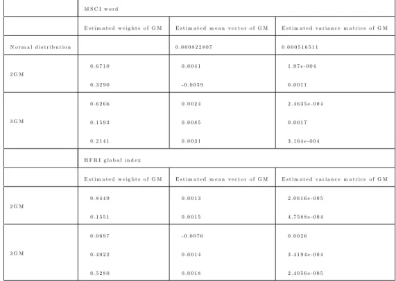
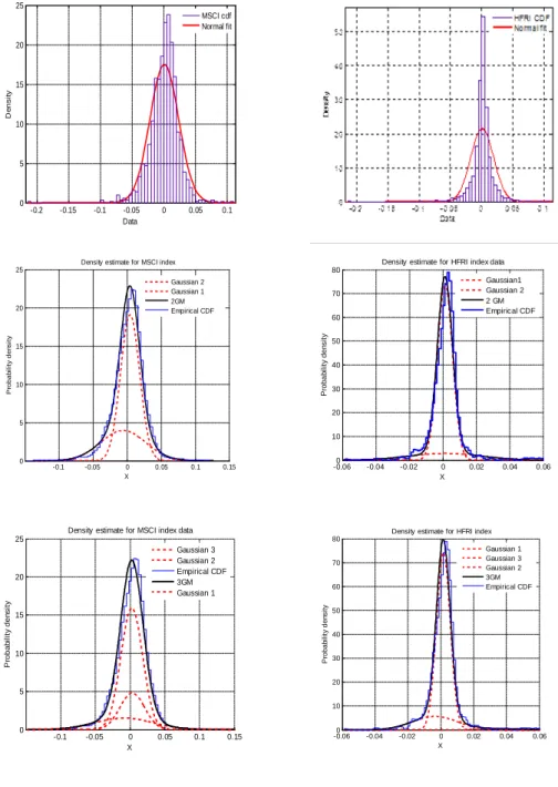
To illustrate Gaussian mixtures, we use the weekly local MSCI world from December 1993 and August 2013 and the weekly HFRX global index, covering the period from January1998 until August 2013. To determine the mixture parameters, we apply the Expected Maximization (EM) algorithm based on Dempster et al. (1977). We investigate two cases: the two mixture distribution and the three mixture one.Next table provides the estimation of the mixture parameters for both …nancial indices. In all the cases, there exists at least a Gaussian distribution with negative mean and another one with positive mean. For the three mixture case, one explanation is that there exist three regimes: the …rst one corresponds to potential signi…cant losses (for example, due to a …nancial crash), the second one to standard evolution of prices and …nally, the third one to potential rises of the indices.
M S C I w o r d E s t i m a t e d w e i g h t s o f G M E s t i m a t e d m e a n v e c t o r o f G M E s t i m a t e d v a r i a n c e m a t r i c e o f G M N o r m a l d i s t r i b u t i o n 0 . 0 0 0 8 2 2 8 0 7 0 . 0 0 0 5 1 6 5 1 1 2 G M 0 . 6 7 1 0 0 . 3 2 9 0 0 . 0 0 4 1 - 0 . 0 0 5 9 1 . 9 7 e - 0 0 4 0 . 0 0 1 1 3 G M 0 . 6 2 6 6 0 . 1 5 9 3 0 . 2 1 4 1 0 . 0 0 2 4 0 . 0 0 8 5 0 . 0 0 3 1 2 . 4 6 3 5 e - 0 0 4 0 . 0 0 1 7 3 . 1 6 4 e - 0 0 4 H F R I g l o b a l i n d e x E s t i m a t e d w e i g h t s o f G M E s t i m a t e d m e a n v e c t o r o f G M E s t i m a t e d v a r i a n c e m a t r i c e o f G M 2 G M 0 . 8 4 4 9 0 . 1 5 5 1 0 . 0 0 1 3 0 . 0 0 1 5 2 . 0 6 1 6 e - 0 0 5 4 . 7 5 8 8 e - 0 0 4 3 G M 0 . 0 6 9 7 0 . 4 0 2 2 0 . 5 2 8 0 - 0 . 0 0 7 6 0 . 0 0 1 4 0 . 0 0 1 8 0 . 0 0 2 6 3 . 4 1 9 4 e - 0 0 4 2 . 4 0 5 6 e - 0 0 5
Table 1: Gaussian mixture estimates for the MSCI world and HFRX global indices
-0.2 -0.15 -0.1 -0.05 0 0.05 0.1 0 5 10 15 20 25 Data De n s it y MSCI cdf Normal fit -0.1 -0.05 0 0.05 0.1 0.15 0 5 10 15 20 25 X Pr o b a b ility de n s ity
Density estimate for MSCI index Gaussian 2 Gaussian 1 2GM Empirical CDF -0.060 -0.04 -0.02 0 0.02 0.04 0.06 10 20 30 40 50 60 70 80 X Pr o b a b ility de n s ity
Density estimate for HFRI index data Gaussian1 Gaussian 2 2 GM Empirical CDF -0.1 -0.05 0 0.05 0.1 0.15 0 5 10 15 20 25 X Pr o b a b ility de n s ity
Density estimate for MSCI index data Gaussian 3 Gaussian 2 Empirical CDF 3GM Gaussian 1 -0.060 -0.04 -0.02 0 0.02 0.04 0.06 10 20 30 40 50 60 70 80 X Pr o b a b ility de n s ity
Density estimate for HFRI index Gaussian 1 Gaussian 3 Gaussian 2 3GM Empirical CDF
2.3
Portfolio optimization
2.3.1 Buy-and-hold strategy
In what follows, we assume that the risky logreturn has a …nite Gaussian mixture distribution. Its pdf is equal to:
fX(x) = n
X
i=1
i; (7)
where fi is the pdf of the distribution N [mi; i] :Denote i= mi+ 2i:. In
what follows, we assume that the sequence ( i)iis increasing, which is equivalent
to the assumption that the expected returnsRexf
i(x) dx are increasing.
The investor maximizes his expected utility:
M axwsE [U [VT]] ;
where VT denotes the portfolio value at maturity T .We have:
VT = V0 erT + ws eXT erT
The …rst-order condition implies:
E U0(VT) eXT erT = 0
which is equivalent to:
n
X
i=1
Z
iU0 V0 erT + ws ex erT ex erT fi(x) dx = 0 (8)
We illustrate how the optimal solutions corresponding respectively to the Gaussian case and the Gaussian mixture case may di¤er. We assume that both probability distributions have same expectation and variance. Consider for instance the three Gaussian mixture case, usually observed on main equity indices for monthly logreturns. In that case, if the expectation is equal to and
the variance to 2 , then we have necessarily: 1+ 2+ 3 = 1 1ec+ 2e 2+ 3e 3 = 1e2 1 e 2 1 1 + 2e 2 e 2 2 1 + 3e 3 e 2 3 1 = 2 with > 0, i 0 . Denote: Si2= e2 i(e i 1)
From previous relations, we deduce the parameter values 2and 3 as
func-tion of 1. Since we have:
2+ 3 = 1 1; 2e 2+ 3e 3 = 1e 1 We get: 2 = (e 3 ) 1;(e 3 e 1) (e 3 e 2) (9) 3 = (e 2 ) 1;(e 2 e 1) (e 3 e 2)
Finally, the coe¢ cient 1;is given by:
1= 2(e 3 e 2) S2 2(e 3 ) + S32(e 2 ) S2 1(e 3 e 2) S22(e 3 e 1) + S32(e 2 e 1) (10)
Therefore, if there exists a solution ws of Equation 8 in [0,1], then we can
apply the implicit functions theorem. Denote:
F ( 1; ws) = 3 X i=1 Z iU0 V0 V0 erT+ ws ex erT ex erT fi(x) dx ; (11) with 2 and 3 as functions of 1 , from Equation 9 (see Appendix for the
bounds on 1).
We deduce the sensitivity of the optimal weight ws invested on the risky asset since we have:
@wS @ 1 = @F @ 1 @F @wS (12)
Note that the second order derivative of the utility function is negative, since we assume that the investor is risk averse, so that his utility function is concave. Thus,h@F
@wS
i
is negative, which implies that wS is a decreasing function of the weight 1if and only if
h
@F
@ 1
i
is negative. This latter condition indicates if the investor prefers (or not) to invest on mixture distributions that overweight the two Gaussian distributions with higher exponential expectations.
To study the sign ofh@@F1i, we note that: @ @ 1 " 3 X i=1 Z ifi(x) # = 1 (e 3 e 2)g (x) ; where g (x) = (e 3 e 2) f 1(x) (e 3 e 1) f2(x) + (e 2 e 1) f3(x)
Then, the sign ofh@@F
1
i
is the same as: Z
U0 V0 erT + ws ex erT ex erT g (x) dx;
which depends mainly on the parameters of the three Gaussian distributions.
2.3.2 Numerical illustrations
To illustrate previous results, we use data the weekly local MSCI world from from December 1993 and August 2013 and the weekly HFRX global index, covering the period from January1998 until August 2013 (see Section 2).
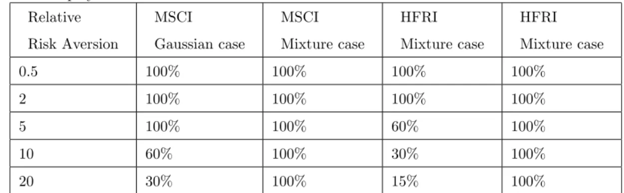
We consider an investor with CRRA utility function given by , where denotes the relative risk aversion. Results for the optimal weight invested on the risky
asset are displayed in Table 2. Relative Risk Aversion MSCI Gaussian case MSCI Mixture case HFRI Mixture case HFRI Mixture case 0.5 100% 100% 100% 100% 2 100% 100% 100% 100% 5 100% 100% 60% 100% 10 60% 100% 30% 100% 20 30% 100% 15% 100%
Table 2: Optimal risky asset weight for the MSCI world and HFRX global indices
For both cases, we note that taking account of mixture models leads to higher investment on the risky asset. A similar result is also true for CARA utility U (x) = ae ax( with a > 0) and for utility with loss aversion as in
Kahneman and Tversky (1992) U (x) = x11 for x < 0 and ( x)1 1 for x < 0 with x < < 1 and > 1). Such empirical examples show that, for a given utility function, there exists signi…cant di¤erences for the optimal portfolio when mixtures are taken into account, even if return expectations and variances are equal.
3
Conclusion
Using Gaussian mixtures allows to …t well empirical distributions. This kind of probability law is commonly used in …nancial modelling, through …nite (regime switching due to economic variables, for instance) or in…nite mixture (Lévy processes, Arch type models...). We show in this paper how it can be possible to optimize a portfolio, in this framework, and in a static way, since portfolio rebalancing takes place in discrete time. The main conclusion is that optimal portfolios for standard Gaussian case and mixture model case can di¤er very sig-ni…cantly, even if the risky …nancial returns have same expectation and standard deviation. Therefore, the mean-variance criterion is a not convenient criterion in the presence of mixture of distributions.
Appendix: Conditions on weights (bounds on 1;)
From Equation 9, we examine now the positivity condition on the weights
i :
1. 0 1 1
2. 0 2 1 () 0 (e 3 ) 1(e 3 e 1) e 3 e 2
This condition is equivalent to: e 2 e 3 e 1 1 e 3 e 3 e 1 3. 0 3 1 () 0 (e 2 ) + 1(e 2 e 1) e 3 e 2 with (e 2 e 1) > 0
This condition is equivalent to: e 2
e 3 e 1 1
e 3
e 2 e 1
Consequently, the positivity condition on the weights i is equivalent to:
M ax 0; e 2 e 3 e 1; e 2 e 2 e 1 1 M in 1; e 3 e 3 e 1; e 3 e 2 e 1
But, since e 1< e 2 < e 3 , we get:
(a) If > e 2; M ax 0; e 2 e 3 e 1; e 2 e 2 e 1 = 0 If > e 3; M ax 0; e 2 e 3 e 1; e 2 e 2 e 1 = e 2 e 2 e 1 (b) M in 1;ee33e 1; e 3 e 2 e 1 = e 3 e 3 e 1
Finally, the positivity condition on the weights i is equivalent to:
(e 2 )+ e 2 e 1 1 (e 3 ) e 3 e 1 . 10
References
[1] References
[2] Alexander, C. (2004): Normal mixture di¤usion with uncertain volatility: modelling short and long term smile e¤ects. Journal of Banking and Fi-nance, 28, 2957-2980.
[3] Alexander, C. and Narayanan, (2009): Option pricing with normal mix-ture returns: modelling excess kurtosis and uncertainty in volatility, ICMA Centre, University of Reading.
[4] Basford, K.E., and McLachlan, G.J. (1985): Likelihood estimation with normal mixture models. Appl. Statist, 34, 282-289.
[5] Basford, K.E., and McLachlan, G.J. (1988). Mixture Models: Inference and Applications to Clustering. New York: Marcel Dekker.
[6] Bellalah, M. and Lavielle, M. (2002): A simple decomposition of empirical distributions and its applications in asset pricing. Multinational Finance Journal, 6, 99-130.
[7] Bellalah, M. and Prigent, J.-L. (2002): Pricing standard and exotic options in the presence of a …nite mixture of Gaussian distributions, International Journal of Finance, 13, 1974-2000.
[8] Brennan, M.J. and Solanki, R., (1981). Optimal portfolio insurance. Jour-nal of Financial and Quantitative AJour-nalysis, 16, 3, 279-300.
[9] Brigo, D., Mercurio, F., (2002): Lognormal-mixture dynamics and calibra-tion to market volatility smiles. Internacalibra-tional Journal of Theoretical and Applied Finance 5, 427-446.
[10] Carr, P. and Madan, D., (2001). Optimal positioning in derivative securi-ties. Quantitative Finance, 1, 19-37.
[11] Dempster, A., Laird, N., and Rubin, D. (1977): Maximum-likelihood from incomplete data via the EM algorithm. J. R. Statist. Soc., B 39, 1-38. [12] Hentati, R. and Prigent, J.-L. (2011): On the maximization of …nancial
performance measures within mixture models. Statistics and Decisions, 28, 1001-1018.
[13] Leland, H.E., (1980). Who should buy portfolio insurance? Journal of Finance 35, 581-594.
[14] Leroux, B.G.(1992): Consistant estimation of mixing distribution, Annals of Statistics, 20: 1350-1360.
[15] McLachlan, G.J. and Peel, D. (2000): Finite Mixture Models. Wiley Series in Probability and Statistics. Wiley.