Edge effects on water droplet condensation

HAL Id: hal-01136630

https://hal.archives-ouvertes.fr/hal-01136630

Submitted on 27 Mar 2015

HAL is a multi-disciplinary open access

archive for the deposit and dissemination of

sci-entific research documents, whether they are

pub-lished or not. The documents may come from

teaching and research institutions in France or

abroad, or from public or private research centers.

L’archive ouverte pluridisciplinaire HAL, est

destinée au dépôt et à la diffusion de documents

scientifiques de niveau recherche, publiés ou non,

émanant des établissements d’enseignement et de

recherche français ou étrangers, des laboratoires

publics ou privés.

Edge effects on water droplet condensation

Marie-Gabrielle Medici, Anne Mongruel, Laurent Royon, Daniel Beysens

To cite this version:

Marie-Gabrielle Medici, Anne Mongruel, Laurent Royon, Daniel Beysens. Edge effects on water

droplet condensation. Physical Review Online Archive (PROLA), American Physical Society, 2014,

90 (6), pp.062403. �10.1103/PhysRevE.90.062403�. �hal-01136630�

Edge effects on water droplet condensation

Marie-Gabrielle MEDICI1,2_{, Anne MONGRUEL}1_{, Laurent ROYON}3_{, Daniel BEYSENS}1,4*

1 _{Physique et Mécanique des Milieux Hétérogènes, UMR 7636 CNRS - ESPCI - Université Pierre et Marie Curie -}

Université Paris Diderot, 10 rue Vauquelin, 75005 Paris, France,

2 _{LPMC Université de Nice, CNRS-UMR 7336, 06108 Nice Cedex 2, France}

3_{Matière et Systèmes Complexes, Université Paris Diderot & CNRS UMR 7057, 10 rue Domont et Duquet, 75205}

Paris, France

4_{Service des Basses Températures, CEA-Grenoble & Université Joseph Fourier, Grenoble, France}

PACS number(s): 68.03.Fg; 68.08.Bc ; 64.60.Q-

*To whom correspondence should be addressed. Email: daniel.beysens@espci.fr; ph: +33140795806. Fax: +33140794522.

ABSTRACT

In this study is investigated the effect of geometrical or thermal discontinuities on the growth of water droplets condensing on a cooled substrate. Edges, corners, cooled/non cooled boundaries can have a strong effect on the vapor concentration profile and mass diffusion around the drops. In comparison to growth in a pattern where droplets have to compete to catch vapor, which results in a linear water concentration profile directed perpendicularly to the substrate, droplets near discontinuities can get more vapor (outer edges, corners), resulting in faster growth or less vapor (inner edges), giving lower growth. When the cooling heat flux limits growth instead of mass diffusion (substrate with low thermal conductivity, strong heat exchange with air), edge effects can be canceled. In certain cases, growth enhancement can reach nearly 500% on edges or corners.

I. INTRODUCTION

Everybody has observed, in a room supersaturated with water vapor, the runoff of water drops condensing on windows. A more careful observation shows that the drops start to flow mostly from the edges of the window. Drops, which are pinned by their contact line on the substrate, detach from an inclined surface when their diameter exceeds a critical size that depends on the inclination angle [1]. The fact that droplets detach sooner from the edge is thus due to their larger size when compared with the other “bulk” droplets. This phenomenon is quite interesting for droplet collection since the top drops can wipe out the entire surface when sliding down.

The reasons of this difference in droplet evolution can be found in the discontinuities of the substrate which modify the water vapor gradient around drops, causing enhancement or reduction of their growth rate. These discontinuities can be either geometric (edge of the substrate, bump, cavity, etc.) or thermal (differences in substrate cooling properties). To our knowledge, no such effects have been reported so far, although drop detachment due to enhanced growth by directed coalescence under wettability gradient has already been observed [2]. It is thus the object of the present study to evaluate the effect of substrate discontinuities on dropwise condensation, the discontinuities being either of geometrical or thermal nature.

II. GROWTH OF A DROPLET PATTERN

A. General

Dew, also called “Breath Figures” (BF) in the laboratory, is the condensation of water vapor on a substrate. The preliminary research on BFs dates back to the years from 1893 to 1922 [3-5]. Fundamental laws of nucleation and growth of BFs were identified later [6-7] and well-characterized regimes were evidenced. The substrate on which condensation takes place is assumed to be maintained at constant temperature. In this study water drops exhibit contact angles θaround 90° with all the investigated substrates of this study, with one exception. Unless specified, we will thus assume in the following that droplets are hemispherical. Four different stages of growth can be identified. (i) Droplets nucleate. (ii) Droplets grow with rare coalescences corresponding to low surface coverage.

The radius, R, of the droplet spherical cap varies with time, t, according to a power law 𝑅~𝑡!. The exponent value depends on the relative values of droplet inter-distance <d>, defined as the mean distance between two neighboring drops centers, compared to the water concentration boundary layer, ζ. The latter measures the extension of the water vapor concentration profile around the droplets. After nucleation, in stage (ii), drops are far apart from each other. It corresponds to <d> > ζ where drops grow independently in a hemispherical profile centered on each drop, resulting in α =1/2. Later on, drop surface coverage increases and drop inter-distance decreases until <d> < ζ. The concentration profiles overlap, the mean profile is directed perpendicularly to the substrate and α =1/3 (a full discussion is given below). (iii) Then droplets touch each other and coalesce, leading to a constant surface coverage and a self-similar growth behavior. The concentration profiles still overlap with the mean profile directed perpendicularly to the substrate and α =1/3 for each individual drop. The mean radius of the droplet pattern grows as < 𝑅 > ~𝑡! _{with γ = 3α. The surface coverage, 𝜀}!_{, being constant at this stage, implies that < 𝑑 > scales with} < 𝑅 > . For instance, hemispherical droplets on a square lattice show a surface coverage 𝜀!_{= 𝜋}!!!!

!!!_! ≈ 0.55. Then

at some time, < 𝑑 > > ζ and nucleation of new droplets can occur between neighboring drops. This is stage (iv). The new droplets which have nucleated then follow the same growth law behavior as described earlier. Further on (stage v), gravity effects become important. The influence of gravity can be measured by comparing the drop radius to the water capillary length 𝑙!= _!∆!! (≈ 2.7 mm with σ ≈ 73 mN.m-1 _{the water-air surface tension, g ≈ 9.81 m.s}-2

the earth acceleration constant and ∆𝜌 = ρw - ρa ≈ 1000 kg.m-3 the air-water density difference). Drops on an inclined

substrate slide down when their weight becomes larger than their capillary pinning forces.

Let us now consider the details of the growth of a droplet when its temperature, Ts, is maintained constant in a

humid air at given temperature Ta and vapor pressure p∞. A sessile drop (contact angle θ) grows by incorporation of

the diffusing water vapor molecules (monomers) around it. The concentration of monomers, c(r, t), counted in mass per volume, obeys the following equation (r is the distance to the drop center):

!"

!"+ ∇. 𝚥 = 0 , (1)

where

𝚥 = −𝐷∇𝑐 , (2)

is the diffusive flux of monomers (mass per unit surface and unit time) with D the diffusion coefficient of the monomers in air.

The problem governed by Eqs. (1–2) is a Stefan problem with a moving boundary at r = R(t). Analytical solutions are rare. For the present problem one assumes a growth slow enough such that the time dependence of c can be neglected in Eq.(1) (quasi-static approximation). Thus Eqs. (1) and (2) reduce to the Laplace equation:

Its solution has to fulfill the following boundary conditions: (i) c(r = R) = cs, corresponding to the water saturation

pressure at the drop temperature, ps, and (ii) c(r → ∞) = c∞, corresponding to the water pressure at air temperature,

p∞. Practically, c∞ (p∞), resp., represents the monomer concentration (water pressure) resp., at the border of the

concentration boundary layer, ζ. It is then assumed that the transport of water molecules towards the droplet surface occurs by molecular diffusion only, i.e. the convective transport is negligible. This will be discussed in section IV-E. The above assumption (i) implies that droplets are isothermal. This can be ensured for the smallest drops where heat transfer occurs on a small (µm) lengthscale. For larger drops, Marangoni thermocapillary convection provides fast heat transfer to make droplets isothermal [8]. Such convective flows have been observed. They provide efficient heat transfer from the drop surface to the condensing substrate and validate an isothermal drop.

Once the concentration of monomers is known, the drop volume evolution can be obtained following the growth equation: !" !" = ! !_! 𝚥 𝑟 = 𝑅 . 𝑛  𝑑𝑆

     

= ! !_!𝐷 ! −∇𝑐 !. 𝑛𝑑𝑆 ! . (4)

Here 𝚥 𝑟 = 𝑅  is the flux of monomers at the drop surface, 𝑛  is the unit vector locally normal to the drop surface, V=π f(θ)R3 _{is the drop volume with 𝑓 𝜃 =}!!!!"#$!!"#$!

!!"#$! and S is the surface of drop/air interface.

Depending whether one deals with a single drop or a droplet pattern, the drop evolution is different. In the following we address these two kinds of growths.

B. Single drop growth

For a single sessile drop on a surface kept at constant temperature, a simple way to solve the problem is to assume an inverse process to evaporation [9-10]. It is implicitly assumed that the probability of incorporating the monomers is uniform on the drop surface, which means that the latent heat of condensation is uniformly removed.

In a 3D space and for a hemispherical drop (Fig. 1a), Eq.(3) has a hyperbolic solution:

𝑐   =   𝑐!  −   𝑐!  −  𝑐! !_! . (5)

The following growth law can then be derived from Eq.

4:

 𝜌!𝑅! !"_!" =  𝑅!𝐷 !!  !  !_! ! . (6)

The integration of this equation gives the classical evolution

with 𝐴 = 2! !!_!!!!

! (in m 2_.s-1_{) .}

This growth law corresponds to an isolated drop or to a drop in a pattern whose water vapor profile does not overlap with the other drops. The latter case occurs when the inter-droplet distance <d> >> ζ.

C. Individual drop growth in a pattern

Let us consider now an array of drops separated by the mean distance < 𝑑 >  on order or lower than ζ (Fig. 1b). This situation corresponds to the end of stage (ii) or stage (iii) between the coalescence events. The individual water vapor concentration profiles merge in a profile parallel to the substrate. The drop pattern can thus be treated as a homogeneous film with average thickness ℎ =!_!!

! =

!_!

!!!! [6-10]. Here 𝑉!   = 𝑉!= 𝜋𝑓(𝜃) 𝑅!

!

is the total condensed volume and 𝑆!  is the surface area of the condensation substrate. Each individual drop (i) with volume Vi

= πf(θ )𝑅!! is assumed to grow like a thin film, where the vapor concentration profile depends only on the normal to the substrate (z axis). Eq. 4 gives a linear variation for the water vapor profile. The boundary conditions are cs =

c(z=h) and c∞ = c(z=h+ζ), where ζ is the concentration boundary layer. (A discussion about its calculation and how

its value impacts the calculation of the drop growth rate is given below in section IV-E). One thus finds:

𝑐   =   𝑐_!+   𝑐_!  −  𝑐_! !!! ! . (8) It follows: h=Bt, (9) with 𝐵 =  ! !_!!!!! !!  (in m.s -1_).

This implies that Vi is proportional to h , and hence, to t. Finally, Ri is proportional to tβ, with β=1/3.

D. Drop pattern evolution with coalescence

In the self-similar growth stage (iii) drops touch each other and coalesce, which leads to an acceleration of the drop pattern evolution. When accounting for such coalescence events, the mean radius evolution of the droplet pattern is rescaled from the individual drop growth Eq.(9) as

𝑅!   =   𝐵!𝑡! , (10) with [6]

𝛾   = 𝛽 !!

!_!!!_! . (11)

Here 𝐷!  (𝐷!) are the drop (substrate) dimensionalities. For 3D droplets growing on a 2D substrate, 𝛾   = 3𝛽 = 1. For 3D droplets growing on a line, 𝛾   =!_!𝛽 = 1/2[11].

In this growth stage where the drop surface coverage is constant, one notes the relation of proportionality between the mean radius of the drop pattern, <R>, and VT. Let us consider the definition of the drop surface coverage

𝜀!₌!!

!_!= ! !_!!

!_! . (12)

Here 𝑆!   = 𝜋 𝑅! is the surface area covered by drops. By expressing the mean drop radius in terms of third and second moments, < 𝑅 >= !_!!! ! !, one gets < 𝑅 >= ! !!_!(!) !! !! = ! !!_!(!)ℎ . (13)

From Eq.(9), one obtains:

 < 𝑅 >  = 𝑘𝑡, (14) with

𝑘 =_!!_!(!)!

! !_!  !  !_!

!!_! . (15)

An evaluation of ζ is given below in section IV-E. It can be used to evaluate k. It is worthy to note that the quantity 𝑐_!  −  𝑐_! /  𝜁 represents the mean water vapor concentration gradient on a drop according to Eq. (4). Eq. (15) can thus be alternatively written as (S is the drop/air interface)

𝑘 = ! !!_!(!)!!

!

! ! −∇𝑐 !. 𝑛𝑑𝑆. (16) In [12] the relation ε2 ≈ 1− θ (deg.)/200 was found between the drop surface coverage and contact angle θ . This

relation stems from the drop coalescence process. When two drops coalesce, the new composite drop exhibits a contact angle, θ, lower than the receding angle, θR . It results a force ∼σ (cosθ - cosθR) that moves the contact line

against the pinning forces. This force decreases as the contact angle diminishes. Then the contact line remains pinned at some places. It results an increase in drop surface coverage when compared to the case where the contact line moves freely. It thus follows from this relation that the mean droplet radius of the pattern grows linearly with time with a prefactor that depends only on the water vapor supersaturation Δ𝑐 = 𝑐!  −  𝑐!, the concentration boundary layer thickness 𝜁 and the vapor in air diffusion constant D. One notes that this growth law remains valid as long as the film approximation remains valid, that is, the individual concentration profiles of drops overlap. It is thus also valid for droplets growing on a 1D, linear substrate and corners.

E. Effects of discontinuities

All the above growth laws are concerned with a uniform substrate corresponding to a semi-infinite medium and drop interfaces maintained at constant temperature thanks to a thermal connection to a thermostat. The latter corresponds to a heat conductive substrate where the latent heat flux coming from condensation can be continuously sent to the thermostat. Growth is then not limited by the heat flux in the substrate. This is generally true when the

substrate is made of a conductive metal in contact with a thermostat, bare or coated with a thin sheet of low conductive materials (polymers). It is not the case when the heat flux limits condensation, e.g. for substrates made of a thick isolating materials or a thin foil not or weakly connected to the thermostat. The growth of natural dew, where the substrate cooling is a balance between surface radiative cooling and air heating, is a more complex case where mass diffusion and thermal diffusion compete. We will thus not consider here this situation.

In this aspect, two types of boundaries can be considered: (i) geometric discontinuity without cooling heat flux limitation as e.g. the boundaries of the condensation substrates and (ii) thermal discontinuities as e.g. the border between a conductive and nonconductive support. (Discontinuities in contact angles are not considered here). Both geometrical and thermal discontinuities have in common a modification of the water concentration profile and thus of the droplet evolution near the border. One can already anticipate that thermal discontinuities and geometrical discontinuities at outer edges will speed up the growth because more water vapor can be collected at the border, whereas geometrical discontinuities at inner edges, where less water vapor is collected, will lower the droplet growth.

A quantification of the effect of borders on drop evolution needs to consider several factors. One notices that drops near discontinuities always undergo coalescence with the neighboring drops that grow on the same plane. As the advancing contact angles are less than 98° (Table 1), there are no coalescences between orthogonal planes.

Let us first consider the drops near a linear edge. Such drops can coalesce with the other drops sitting in a half-plane. The edge drops can thus be considered as particular drops of the same plane but with a vapor concentration profile that is now two-dimensional. Observation (Figs. 2-3) shows that the corresponding drop pattern exhibits the features of scaling during growth: uniform radius, drop inter-distance on the order of the radius. Such scaling can be verified by the constancy of the drop surface coverage 𝜀!=! !!!

!_! during drop pattern evolution. The summation is made on the edge condensing surface, SE. The latter is not constant during evolution. Its determination can be

performed by making use of а method based on Voronoi polygons or Dirichlet tessellation [13]. Such а polygon is the smallest convex polygon surrounding а drop whose sides are the bisectors of the lines between the drops and its neighbors. The edge surface can thus be considered as the total surface of the Voronoi polygons of the edge drops (Fig. 4c).

Note that a good approximation of the ε2 _{calculation can be obtained from the evaluation of the line surface}

coverage of the edge drops, 𝜖!=! _!!!. The summation is made along the edge of length L removing the two corner drops. The edge surface can then be considered as a band of length L and constant width w, corresponding to the mean extent of the Voronoi polygons perpendicular to the edge. From the Voronoi construction, w=α<R>, with α a proportionality constant on order two. One thus obtains ST∼L<R> and 𝜖!=

! !!!

∝!!!!. Making use of the evaluation < 𝑅 >= !!!

!

! , one readily obtains 𝜖

!₌ ! !! 𝜖

!_{. Results are reported in Fig. 4a for substrate P1 and Fig. 4b for} substrate P2. Constant surface coverage is found for the edge zone with both ε2 (= 0.56 ± 0.02 for P1) and ε1 (= 0.78 ± 0.01 for P1 and 0.71 ± 0.01 for P2). From the ratio ε2/ ε1 one determines α = 2.1 ± 0.1, the expected value.

< 𝑅 >= !!_!!_!

! . (17)

The vapor concentration profiles of the edge drops overlap, then the assumption of equivalent film holds and 𝑅!_~𝑉

!,!~𝑡

! , with VT,E the condensed volume near the edge. One thus eventually gets the growth law <R> = kE t,

similar to Eq. (14), however with a different prefactor kE corresponding to a different mean vapor profile on the

drops. In the equivalent film approximation, one has two perpendicular linear profiles, one directed perpendicular to the condensing plane, the other perpendicular to it.

Note that growth near a linear edge is different from 1-D growth (as e.g. drops growing on a very thin thread) where line coverage ε1 _{is constant or 𝑅 = constant. In this case Eq. (13) can be rewritten as < 𝑅 >=} !!

!!=

!!

! !

!! . The first term is proportional to the condensed volume VT ∼t and the second is 1/<R>, giving <R>∼t1/2.

Let us now consider the case where the edge is a corner. This case is not so much different from the linear edge case, although there is only one drop growing at a corner. The corner drop can be considered as a particular drop of a linear edge with a vapor concentration profile that is now three-dimensional.

This drop undergoes coalescence with other drops from two different edges and drops from the plane (see Fig. 2), leading to constant surface coverage (= 0.62 ± 0.02, see Fig. 4a). Then the film approximation holds and growth still follows Eq.(14).

The estimation of the gradient near the edge depends on the particular edge geometry and needs to solve the Laplace equation, Eq. (3). A theoretical estimation is out of the scope of the present study. The solution for a 2D arrangement will be performed numerically in the next section V. In order to highlight the vapor pressure dependence of the gradient, one defines a new mean boundary layer thickness, 𝜁!, such as (Eq. (4)), !

! ! ∇𝑐 !. 𝑛𝑑𝑆= !_!  !  !_!

!_! (Sis the drop-air interface). Equations (14-15) can thus still hold for a droplet pattern near a discontinuity, with a new factor 𝑘!:

𝑘_!= ! !!_!(!)

! !!  !  !!

!!!! . (18)

This factor is different according to the type of discontinuities.

III. MATERIALS AND METHODS

Condensation experiments are performed on a cooled horizontal substrate in order to get rid of the droplets detachment and sliding along the substrate. The study is limited to drops size lower or on the same order than the water capillary length . It corresponds to having negligible gravity effects on the shape of the drop.

A. Condensation chambers and observation set up

Two different test chambers and optics are used, depending on the length scale investigated.

c

Experiment type 1. For small droplet size (range 5-100 µm), the growth process is observed from above with a high resolution CCD color camera PixeLink (PL B776F) connected to a computer. This camera is equipped with a Pentax Megapixel lens with a 6 mm focus length to get a ×8 magnification at 5 cm from the substrate (30 px/mm). The latter is put on an electrolytic copper block cooled by a Peltier element. The thermal contact is ensured either by a small layer of water or by thermal grease (a silicone-free heat sink compound). Dew condenses from the room ambient air whose temperature Ta and air relative humidity RH is constant during the experiment time within ± 0.5

°C and 3%, respectively. The temperature of the substrate is measured by a thermocouple taped on it.

Experiment type 2. For larger droplets (typical range 0.1-5 mm), the above arrangement is enclosed in a large Plexiglas chamber, where air temperature and RH is maintained constant. The same optical system as for experiment type 1 is used, however the distance between the substrate and the lens is larger (14 cm) giving a magnification of 42 px/mm. The substrate holder is a 2 mm thick stainless square steel plate of 173.2 x 173.2 mm size, screwed with thermal grease on a electrolytic copper plate of same size in contact with a Peltier element thermostat. The hot side of the latter is cooled by a fan directed on a water basin, which ensures large and stable air humidity ( RH >76%) and temperature. Air and surface temperatures together with humidity data are recorded by a data logger (Testo 454) coupled to a computer.

Although the characteristics of humid air can be monitored, it is not possible to control in each experiment the exact conditions of air flows around the substrate. To get rid of this uncertainty, the evolution of droplet radius at the substrate boundaries will be rescaled by the corresponding droplet radius evolution in the central part of the substrate. Both evolutions are expected to be linear according to section II-E.

The images are analyzed with an image analysis software (ImageJ) to obtain the mean surface of the droplets in a given image area. The radius is that of a spherical cap seen from above. The uncertainties in the drop radius measurements correspond to (i) optical resolution, from 0.4% for large (mm) drops to 4% for the smaller (0.1 mm) drops, (ii) number of drops for calculating the average, which gives smaller uncertainties for small drops than with large drops, (iii) irregularities of air convection. The uncertainties (i) and (ii) compensate to give an overall uncertainty of about 4%, whereas the uncertainty (iii) is difficult to estimate. We decided to report in the figures the error bars corresponding only to the uncertainty of measurements (4%). In the fitting procedure, we report the statistical uncertainty corresponding to two standard deviations (95% confidence). In total, 37 sets of experiments have been performed. The reproducibility is on order of 10% when droplet evolution at the boundaries is rescaled by the corresponding evolution in the center of the substrate (see section IV and Table 2).

B. Condensation substrates

Different substrates are used to evidence various types of discontinuities.

Experiments type1: (a) A brass rectangular parallelepiped (P1 substrate, Fig.2a) of 17.5 mm height, top surface of 15.1 mm x 10 mm is covered by an adhesive grey foil of polyvinyl chloride (PVC) with 0.14 mm thickness. This sample provides a geometrical discontinuity of corner and linear edge type. (b) Two aluminum alloy (duralumin) massive triangles (P2 substrate, Fig. 2b), separated by a gap, forming a diamond, are covered by an adhesive brown foil of polypropylene (PP) with 0.02 mm thickness. In addition to geometrical discontinuities, two thermal discontinuities are present along the gap between the triangles where the foil cannot be cooled.

Experiments type 2: Geometrical discontinuities are realized in different type of materials with different wetting and thermal properties. (i) A square duralumin plate (G1 substrate, Fig. 3a), 2 mm thickness and 173.2 mm side (same size as the substrate holder) provides different kind of geometrical discontinuities: U-groove at 40 mm from the left edge (width: 10 mm, depth: 1 mm) and a linear scratch of about 0.1 mm depth in the center of the plate. (ii) A 0.1 mm thick PP foil (G2 substrate) is stuck with a thin water layer on the above duralumin substrate. Only corner and linear edges were concerned with this coating, not the groove. (iii) A polymethyl methacrylate plate (G3 substrate, commercial name Plexiglas), with the same geometrical characteristics than the above G1 substrate. It is stuck on the substrate holder with a thin water layer.

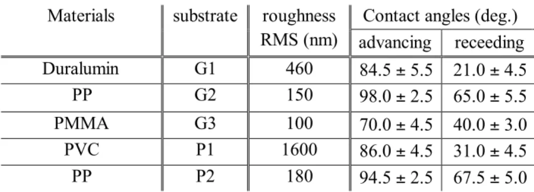
The roughness of the above substrates is the same on the flat and on the edge regions and has been measured by an optical profilometer. The results are reported in Table 1. The mean contact angles on water on the above substrates have been measured by two methods, looking at the shape of the drop on (i) an inclined substrate at the sliding onset and (ii) when pushing or pulling water on a horizontal substrate with a syringe. The results are the same within the uncertainties. The mean values for both methods are reported in Table 1. These values are typical of substrates used in the open air or an industrial environment and ensure dropwise condensation. Except for PMMA, the advancing contact angles are close to 90°. The hysteresis of the contact angle is correlated with the surface roughness, as expected.

IV. OBSERVATION AND ANALYSES

We comment in the following the different evolutions corresponding to the different types of discontinuities (corner, edge, groove, scratch, thermal). Condensation proceeds on a very long time period corresponding to the stage (iii) of the self-similar growth (Figs. 2 and 3). Then the short time periods of the nucleation phase (i) and the individual growth stage (ii) can be neglected. In the center of a 2D substrate the evolution of the drop mean radius can thus be fitted to a linear growth law, consistent with Eq.(14). From Eq. (15), this prefactor k is proportional to the supersaturation Δ𝑝 = 𝑝!  −  𝑝!and the water vapor diffusion constant in air, D. It is inversely proportional to the concentration boundary layer thickness, ζ. As discussed in section II-E, the effect of discontinuity does not change the mean droplet growth law on the discontinuity, only the prefactor k is modified into 𝑘!.The experiments, which have been performed under different conditions of temperature (Ta, Ts), give different boundary layer

thicknesses and different condensation parameters RH or Δ𝑝. For comparison and discussion, the growth rates 𝑘! at different locations (E) are thus rescaled by the value, kM, measured at the central, middle part (M) of the substrate,

corresponding to the same parameters (air flow, Ta, Ts, RH, and Δ𝑝). The ratio

!_! !_!=

!_!

!_!, with ζE, ζM the mean

boundary layer thickness at E, M, locations can thus be compared without accounting for the different experimental conditions. With such a rescaling, the reproducibility of experiments remains within 10%. This ratio is listed in Table 2 and discussed for the different experiments in section VI.

In the following we report the different growth laws for the substrates as described in section II.

In Fig. 2c is reported a photo of water condensation on P1 substrate. The drops on corner and linear edges exhibit clearly larger sizes than the drops close to but apart from the discontinuities.

Seven sets of experiments have been performed. A typical evolution of the mean drop radius on corners, edges and the central region is reported in Fig. 4a. The values are averaged on the 4 edges and corners. As expected, it is observed that droplet growth is faster at the substrate corners than at the edges, the latter giving faster growth than in the central region. A fit to Eq. (14) with k as adjustable parameters give kC = (12 ± 0.4) 10-3 mm/min (average on

four corners), kE = (8.3 ± 0.2) 10-3 mm/min (edges), kM = (3.52 ± 0.04) 10-3 mm/min (central region). The ratios to the

central region are reported in Table 2.

B. Edges and thermal borders on P2 diamond

In Fig. 2d is reported a photo of water condensation on P2 substrate. The drops on thermal and geometrical corner and linear edges exhibit clearly larger sizes than the drops close to but apart from the discontinuities.

One set of experiments has been performed in this configuration. In Fig. 4b are reported the evolution of the mean drop radius on edges, border of the thermally inhibited condensation (thermal) and the central region. The values are averaged on all 4 edges and thermal boundaries. As above with parallelepiped P1, it is observed that droplet growth is faster at the substrate edges than in the central region. Growth at the thermal borders is faster than in the central region but slower than at the edges. A fit to Eq. (14) with k as adjustable parameters give kE = (5.0 ± 0.2) 10-3

mm/min (edges), kT = (4.1 ± 0.1) 10-3 mm/min (thermal border), kM = (1.8 ± 0.15) 10-3 mm/min (central region). The

ratios to the central region are reported in Table 2.

C. Corner, edge, groove and scratch on G1 and G2

In Fig. 3b is reported a photo of water condensation on the G1 substrate (duralumin). The drops on outer linear edges exhibit clearly larger sizes than the drops close to, but apart from the discontinuities. The drops near the groove, in the upper region, also show larger drops. In contrast, drops near the groove edge in the inner region show smaller drops. The drops in the inner central region of the groove and on the scratch have similar size than in the central region of the substrate.The scratch gives somewhat aligned droplets.

Numerous experiments (24) have been performed on G1. Evolutions of the droplet radius are reported in Fig. 5a for a typical experiment. The radius is averaged on the two upper plate corners, the upper plate edge and the central region. Also reported are the drop radius evolution on the upper edge of the groove, in two locations 1 and 2 (edge groove+ (1) and edge groove+ (2)), the lower part of the groove edges (edge groove-) and the central part of the groove (central groove). The scratch gives somewhat aligned droplets (see Fig. 3b) but their evolution is similar to the central part of the plate. As reported in (6), a scratch induces a 1D growth only in the early stages of growth when the drop diameter is less than the scratch thickness. For larger drop sizes, growth is the same as on a 2D surface.

As above for P1 and P2 droplets grow faster at the substrate corners than at the edges (plate and groove edge), the latter giving faster growth than in the central region. The central part of the groove exhibits a slighter slower growth than the central part of the plate. The lower groove edge gives the slower growth. A fit to Eq. (14) with k as

adjustable parameters give kC = (28 ± 2) 10-3 mm/min (average on two corners), kE = (16.1 ± 0.4) 10-3 mm/min

(edges), kG+ = (9.8 ± 0.4) 10-3 mm/min (groove edges), kM = (6.2 ± 0.4) 10-3 mm/min (central region), kGM = (5.3 ±

0.2) 10-3 _{mm/min (groove central region), k}

G- = (3.2 ± 0.2) 10-3 mm/min (groove lower edge). The ratios to the plate

central region are reported in Table 2. Note that a step-like evolution is visible on the corner drops. These discrete steps are much larger than the experimental error, and reproducible. Each step corresponds to a coalescence event with a neighboring drop. It is a characteristic feature of the corners, where the evolution of a single drop is observed, whereas for the other locations the coalescence events are averaged on a line (edges) or on a surface (middle) ; they remain only barely visible on edges.

The G2 substrate (same as G1 but coated with polypropylene foil), shows the same kind of behavior as on the G1 substrate, although water drops exhibit a larger contact angle (Table 1). Three sets of experiments have been performed. A fit to Eq. (14) with k as adjustable parameters give kC = (80 ± 2.5) 10-3 mm/min (average on two

corners), kE = (46 ± 1) 10-3 mm/min (edges), kM = (15.3 ±0.2) 10-3 mm/min (central region). The growth rates ratios

corresponding to the corners and the edges region are reported in Table 2.

D. G3 low conductive plate

Two sets of experiments have been carried out with the G3 plate. They do not give any of the above observed edge effects as can be seen in Fig. 3c. The drop diameters show the same increase on corners, edges and central part. However, growth is accelerated inside the groove.This striking observation can be understood when considering the quite different values [14] of thermal conductivity, λ, for metallic substrates (duralumin: 160 Wm-1_K-1_{; brass: 120}

Wm-1_K-1_{) and PMMA (0.19 Wm}-1_K-1_{) [15]. The cooling heat flux P per unit surface corresponds to maintain a}

constant temperature at the substrate surface by compensating for air heating (heat flux Pa) and condensation latent

heat (Pc) : 𝑃 + 𝑃!+ 𝑃! = 0 .

One can express the different flux per unit surface as_!!!

!= 𝜆! !!!!! !! and

 

 𝑃𝑐 𝑆_𝑇 = 𝐿 𝑆_𝑇 𝑑𝑚 𝑑𝑡 = 𝐿𝜚𝑤 𝑑ℎ 𝑑𝑡. (19)

Here ρw (= 1×103 kg.m-3) is the density of liquid water,L (= 2400 kJ.kg-1) the latent heat of condensation andλa (=

0.026 Wm-1_K-1_{) the air thermal conductivity [14]. The thermal boundary layer in air, δ}

Τ, corresponds to the

thickness where the transport of heat by conduction becomes more efficient than by convection or a Peclet number PeT=UδΤ/D_T <1 (U is air velocity, D_T = 2.2×10

−5 _m2_.s−1 _{[14] is air thermal diffusivity). Although the thermal}

boundary layer is of different nature than the diffusive boundary layer, which corresponds to the diffusion of water molecules in air, characterized by the diffusion coefficient D, it happens that the value D = 2.4×10-5 _m.s-1 _{[14] is}

Making use of Eq. (9), one obtains _!!!

!= 𝐿

!∆!

! . The flux P can be expressed as the conduction through the substrate of thickness e in contact with the Peltier element at temperature T0,

! !!= 𝜆

!!!!!

! . (20)

In the present experiment where Ta = 25°C, RH = 62%, Ts = 16°C, T0 = 13°C (Δp = 0.20 kPa) corresponding to Δc

= 1.6×10-3 _kg.m-3_{, the ratio air conduction over condensation} !!

!!=

!_!(!_!!!_!)

!"∆! ≈ 2.5. Thus nearly most of the heat flux P/ST (≈ 300 W.m-2)is used for cooling the substrate. From Eqs. (19-20) one can estimate the limiting growth rate

dh/dt ≈ P/(  𝐿𝜚!3.5ST) ≈ 2×10-3 mm/min This is a rough estimation as it is obtained by subtracting two large heat

fluxes. However, the growth rate is on the same order as the rate found in the central part of G3: kM = (4.5 ± 0.2)10-3

mm/min.Drops are seen to grow faster in the groove than on the surface because the conductive cooling heat flux is here more important. With a growth rate in the groove kGM= (7.5 ± 0.6) 10-3 mm/min, the growth rate enhancement

is kGM / kM = 1.7 ± 0.2 (Table 2). This value compares well with the factor 2 that is expected from the cooling heat

flux from Eq.(20), assessing that the droplet growth is indeed limited by the low thermal conductivity of PMMA.

E. Boundary layer thickness and growth rate

The concentration boundary layer thickness ζ corresponds to the extent of the region near the substrate, where the transport of water molecules by diffusion becomes more efficient than by convection. In other words, it corresponds to a Peclet number PeC=Uζ/D <1 (U is air velocity).

One can have a rough estimation of ζ by a scaling analysis of the natural convection above a horizontal cooled plate [16]. Due to buoyancy effects, air flow will be confined in a hydrodynamic boundary layer of thickness δ. The latter is a function of the Grashof number Gr =!"∆!!_!! ! as δ ∼L Gr-1/5_{. Here L (≈ 20mm) is the plate characteristic}

length, ΔT = Ta-Ts, β = 2/(Ts+Ta) = 3.4×10-3K-1 is the air volumetric thermal expansion coefficient (airconsidered

as ideal gas) and ν = 1.6 10-5 _m2_{/s is the air kinematic viscosity[14]. These values give Gr ≈ 13000 and}

δ ≈ 3 mm with ΔT ≈ 10 K. As δ ∼ ΔT0.2, its value is only weakly sensitive to temperature. The maximal velocity in the

hydrodynamic layer is given by Um ~ (δ β g ΔT)1/2 ≈ 3 cm/s [16]. With D = 2.4×10-5 m.s-1 [14] the diffusion constant

of water in air, PeC ≈   3 for U=Um. Assuming that the air velocity decreases near the plate following a parabolic

flow, the boundary layer thickness ζ can be deduced from PeC (z)=  

𝑈(𝑧)𝑧   ! = !!! ! ! !/! ! = 1: 𝜁~ _{! !"Δ!}!!!/!_!/!!/! . (21)

The ζ value is only weakly temperature dependent. For ΔT ≈ 10K, one finds ζ ≈ 1.1 mm. It results that for droplets of radius lower than 1.1 mm, growth remains limited by diffusion. When the drop diameter becomes larger,

a thorough description of the process would need a fine description of the convective flow in the exact experimental configuration.

The above expression of ζ , Eq.(21), can be inserted in Eq. (15) to calculate the growth rate k, whose value can be then compared to the experimental value of km in the central part of the substrate. In the dependence of the surface

coverage with the contact angle, 𝜀!_{=1-(θ (deg.) /200) [12], one has to consider the advancing contact angle as} drops are growing. The values are listed in Table 2. One notes that the kM experimental values are in general

significantly larger than the calculated values and show significant variations, even for similar substrates under same conditions (G1, G2 and P1, P2). In addition to the fact that the calculated values originate from scaling (approximate

estimation, Eq. (21)), variations do exist because of uncontrolled air flows around the substrate. Indeed the experiments were not designed to control air flows (it is a quite difficult task). Hydrodynamics is then not simply natural convection and can vary in an uncontrolled way from experiment to experiment.

F. Condensation on an inclined substrate

In all above-mentioned experiments the substrate was horizontal in order to focus on the edge effects only. In this section we present an example of a condensation experiment on an inclined substrate, in order to show qualitatively the combined action of edge effects and gravity. Figure 6 shows the condensation pattern on a silicon wafer inclined at 30° from horizontal. The droplets situated near the upper horizontal edge have grown faster than their neighboring droplets. As a consequence, they reach sooner the critical size necessary for detachment, and, acting as wipers, collect the other drops as they slide down. The condensing surface is thus continuously renewed, and the condensation process is sustained.

This "self-cleaning" effect should have practical implications on the water collection efficiency of inclined surfaces. It remains, however, to be precisely quantified.As a matter of fact, it has been reported that dew collectors of origami form with many edges can collect up to 400% more water than simple planar surfaces for small dew events [17]. The question arises about spines or sharp needles that are encountered in some plants to favor natural dew condensation and collection. In order to improve water harvest efficiency one could also combine the edge effects of the condensation substrate with the wettability and geometry properties as studied in [18]. A coating with small contact angle hysteresis placed on the upper borders of a condenser should promote the early detachment of small drops, thus enhancing the wiper effect.

V. SIMULATIONS

In the simulation the condensing plate is supposed either perfectly conductive (isothermal) or adiabatic such as only mass diffusion in humid air above the plate matters. We consider a “snapshot” where the droplet configuration is fixed, the size of the droplet are set and droplets are not growing. They are placed in various configurations with different concentration boundary layer geometries. It is also assumed that inside the concentration boundary layer, the transport of the molecules by natural convection is negligible compared to their transport by diffusion (PeC <1).

The validity of this assumption has been assessed above in section IV-E by performing a scaling analysis of the natural convection above a horizontal cooled plate.

This situation thus corresponds to solve only the diffusion equation in a stationary state. As a result of the calculation, the drops are receiving a mass flux that characterizes their rate of growth during the snapshot small time interval in this fixed configuration.

A. Model geometry and boundary conditions

The comparison of the growth rates of drops at different geometrical and thermal boundaries is inferred from the value of the mean water vapor concentration gradient at the drop perimeter, Eq. (4). To calculate this value, we solve the steady state diffusion equation Eq. (3) in two dimensions (2D) for water vapor concentration c : Δc = 0, using a finite element method implemented in Matlab (pdetool). A 2D simplification is consistent with the fact that the droplets close to edges are aligned (see Figs. 2-3). It is not, however, the case for the droplets at the corners and is a simplification for the central part.

The geometry of the domain is depicted in Figs. 7ab. The boundaries of the domain are (i) the solid surfaces of the substrate where drops are growing and (ii) the surface boundaries where water vapor concentration is kept constant. These surfaces correspond to the position of the concentration boundary layer as estimated previously in section IV.E. The values that are used in the simulation ( 1 and 2 mm) are typical of the boundary layer thickness.

We address two substrate geometries, an edge (Fig. 7a) and a groove (Fig. 7b), to mimic the geometry of the AL plate (Fig. 3). On the substrate, hemispherical drops of same diameter 2R = 200µm are distributed with a distance between the edges of two neighboring drops equal to 50µm). It means that each drop is at the center of a box of width d = 250 µm, corresponding to a mean interdrop distance <d> = d. This configuration correspond to a drop surface coverage ε2 _{= 0.50, as observed during the coalescence – driven, self-similar coalescence stage (iii). The}

drops are situated within a distance of 50 µm from the boundary.

For the edge case, the thickness of the substrate is set to 2 mm. On the substrate walls between the droplets, we impose a zero transversal flux, i.e. a zero concentration gradient. Symmetry dictates that on the boundaries X = 3 mm and Y = 0 mm, the transversal flux is zero. On the boundaries Y = 3mm and X = 0, a uniform concentration c∞=

2 (in arbitrary units) is imposed. These surfaces are situated at a distance of 1 mm from the substrate, corresponding to the case ζ >> <d>. On the drops surfaces, a saturated concentration cs =1 is assumed. This yields a ratio 𝑐!/cs

typical of the ratio (p∞/p_s) used in the experiments. In Figs. 7ab,the local diffusive flux vectoris depicted as arrows,

the colors represent the intensity of the local concentration gradient. The maximal concentration gradient intensity is found at the surface of the droplets situated close to the edge E, and a decreasing concentration gradient is observed with increasing drop distance from the edge.

The groove (Fig. 7b) is 1mm in depth and 4 mm in width. For symmetry reasons, we simulated only half of the groove. As for the edge, the concentration is set to c∞= 2 at Y = 1mm from the substrate. The concentration is set to

cs = 1 on the surface of the drops. In agreement with the preceding cases, the concentration gradient amplitude is

maximized on the drop G+ situated at the edge of the groove. In contrast, it is the smaller for the drops inside the groove, with decreasing values from the inner groove edge G- towards the inner groove middle GM.

A thermal border is shown in Fig. 7c where the boundary (Y = 0, X<1mm) corresponds to an adiabatic substrate where drops cannot grow. As for the edge and the groove, the concentration is set to c∞= 2 on the surface at Y =

2mm, situated at 1mm from the top of the substrate. The concentration is set to cs=1 on the surface of the drops. The

transversal concentration gradient is set to zero on the symmetry axis X = 0, on the solid surfaces of the substrate, and on the boundary (Y = 0, X<1mm).

It can be seen on Fig. 7c that similarly to the preceding cases, the concentration gradient is maximized on the drops situated at the edge of the (thermal) boundary T. It decreases towards the middle M of the drop pattern.

B. Comparison with experiments

Following Eqs. (2, 4) for the monomer flux and drop volume evolution dV/dt, we thus compute the following integral :

𝐼 =!_{! !} ∇𝑐 _!. 𝑛𝑑𝑆 , (22)

of the concentration gradient on the different individual drop surfaces to determine a quantity which is proportional to the mean drop volume growth rate dV/dt(Eq.(4)) and thus to d<R>/dt = k from Eq.(16).  

In order to compare with the experiments, the integral of the concentration gradient is computed on drops marked on Fig. 7, M (central part of the substrate), E (edge), G+ (outer edge of the groove) G- (inner edge of the groove), GM (central part of the groove), T (thermal discontinuity).

The ratio of each integrals I to the integral IMcorresponding to the substrate central is independent of the value of

the vapor diffusion coefficient D and of supersaturation, see Eqs. (15 -18). It is listed in Table 2 where it can be compared to the corresponding experimental values kJ /kM . The values compare relatively well taking into account

the fact that the simulation is 2D. There is one exception concerning kG-/kM (the groove inner edge) where the

calculated value is 7 times lower than the measured value. This discrepancy is due to the assumption in the simulation of the boundary layer above the groove. In the reality, the layer should curve towards the groove, thus enhancing the growth rate.

VI. CONCLUDING REMARKS

From this study it appears that droplet growth on a cooled substrate can be significantly modified by discontinuities. They can be of geometric or thermal nature and growth can be enhanced or reduced. In the case where mass diffusion around the drops controls growth, drops can collect more or less moisture near a boundary than in the middle of the substrate depending on the shape and nature of the discontinuity. In certain cases, the growth enhancement can reach nearly 500% on edges or corners.

On the other hand, these boundary effects can disappear when another process than mass diffusion limits growth. This is for example the case for substrates where the cooling heat flux is limited by the low thermal conductivity of

the substrate (PMMA substrate in this study) or strong heat exchange in a windy atmosphere when cooling is ensured by radiation deficit (natural dew).

ACKNOWLEDGMENTS

We gratefully thank Martin Hendel for his valuable corrections and for his critical reading, helpful remarks and relevant comments.

REFERENCES

[1] B. Krasovitski and A. Marmur, Langmuir 21, 3881 (2005). [2] D. Susan, M. Chaudhury, and J. Chen, Science 291, 633 (2001). [3] J. Aitken, Proc. R. Soc. Edinburgh 20, 94 (1893).

[4] A.L. Rayleigh, Nature (London) 86, 416 (1911). [5] T. Baker, Philos. Mag. Series 6, 44, 752 (1922).

[6] D. Beysens, Comptes Rendus Physique 7, 1082 (2006), and refs. therein. [7] B. J. Briscoe and K. P. Galvin, Phys. Rev. A 43, 1906 (1991).

[8] J. Guadarrama-Cetina, R. D. Narhe, D. A. Beysens, and W. Gonzalez-Vinas, Phys. Rev. E 89, 012402 (2014).

[9] R. G. Picknett and R. Bexon, J. Colloid Interface Sci. 61, 336 (1977).

[10] M. Sokuler, G. K. Auernhammer, C. J. Liu, E. Bonaccurso, and H.-J. Butt,EuroPhys. Lett.89, 36004 (2010).

[11] A. Steyer, P. Guenoun, D. Beysens, D. Fritter, and C. M. Knobler, EuroPhys. Lett. 12, 211 (1990). [12] H. Zhao and D. Beysens, Langmuir 11, 627 (1995).

[13] A. Okabe, B. Boots, and K. Sugihara, Spatial Tessellations Concepts and Applications of Voronoi Diagram (John Wiley & Sons, New-York, 1992).

[14] CRC Handbook of Chemistry and Physics, 79th ed., (edited by D. R. Lide , CRC Press, Boca Raton, FL, 2006).

[16] K. Gersten and H. Herwig, Strömungsmechanik, Grundlagen der Impuls-, Wärme- und Stoff-Ubertragung aus Asymptotischer Sicht, (Vieweg, Braunschweig-Wiesbaden, 1992).

[17] D. Beysens, F. Broggini, I. Milimouk-Melnytchouk, J. Ouazzani, and N. Tixier, Chemical Engineering Transactions 34, 79 (2013).

[18] A. Lee, M.-W. Moon, H. Lim, W.-D. Kim, and H.-Y. Kim, Langmuir 28, 10183 (2012).

TABLES

Table 1. Surface roughness (root mean square RMS) of the materials with contact angles of water.

Table2. Values of radius growth rate kMon substrate central region (exp.: experimental value; calc.: calculated from

Eq. (15)), kE (substrate edge). Comparison is also given between the experimental ratios kE/kM (overall uncertainties

are within 10%) and the simulated ratios I/IM. Δp is the difference p∞ - pS (see text). The values under brackets for

G3 [(1) and (2)] correspond to the ratio of heat fluxes for low conductivity PMMA substrate. The missing data correspond to non-existent geometries in the simulation or in the substrates.

Materials

substrate

roughness

RMS (nm)

Contact angles (deg.)

advancing receeding

Duralumin

G1

460

_{84.5 ± 5.5 21.0 ± 4.5}

PP

G2

150

_{98.0 ± 2.5 65.0 ± 5.5}

PMMA

G3

100

_{70.0 ± 4.5 40.0 ± 3.0}

PVC

P1

1600

_{86.0 ± 4.5 31.0 ± 4.5}

PP

P2

180

94.5 ± 2.5 67.5 ± 5.0

G1

G2

G3

P

1

P

2

I/IM

kM

(10-3 _mm.min.-1₎

exp.

6.2

15.3

4.5

3.5

1.8

calc.

22

9.0

6.7

11.4

9.8

kC

/k

M

4.6

5.2

1 (1)

3.4

-

-

kE

/k

M

2.6

3.0

1 (1)

2.4

2.7

1.90

kG+

/k

M

1.6

-

1 (1)

-

-

1.66

kGM

/k

M

0.86

-

1.7 (2)

-

-

0.43

kG-

/k

M

0.51

-

1.7 (2)

-

-

0.072

kT

/k

M

-

-

-

-

2.2

2.64

Ta (°C)

25

23

25

22.6

22.6

Ts

(°C)

15

12.5

16

4.8

4.8

RH (%)

78

76

62

44

44

Δp (kPa)

0.80

0.40

0.20

0.35

0.35

FIG. 1. (Color online) Schematics of different regimes for the droplet growth on a substrate : (a) single drop evolution ;(b) growth in a pattern with overlapping water vapor concentration profile, and film of average thickness h.

c

_∞

_,

   

p

_∞

c

_s

_{,  p}

_s  

r

r  =  ζ

R

(a)

(b)

c

_s,

p

_s

Z

z  =  h+ζ

z  =  h

<d>

R

_i

c

_∞

_,

   

p

_∞

(b)

FIG. 2. (Color online) Substrate geometries and condensation patterns in experiment type 1 (see text). (a) Schematic of substrate P1: PVC foil on brass parallelepiped . (b) Schematic of substrate P2: PP foil on duralumin diamond. (c) Condensation on P1 (28 min, Ta = 25.9°C, RH = 59%, Ts = 7.7°C). (d) Condensation on P2 (26 min 40 s, Ta =

22.6°C, RH = 44%, Ts= 4.8°C).

(b)

(a)

8 mm

7 mm

35 mm

35 mm

10 mm

15.1 mm

17.5 mm

 

 

(c)

(d)

FIG. 3. (Color online) Substrate geometries and condensation patterns in experiment type 2 (see text). (a) Schematic of G1, G2 and G3 substrates. (b) Condensation on G1 (120 min; Ta = 25°C, RH = 78%, Ts = 15°C). (c) Condensation

on G3 where growth is limited by the cooling heat flux (240 min, Ta = 25°C, RH = 62%, Ts = 16°C).

(a)

(c)

(b)

173 mm

40 mm

10 mm

1 mm

2 mm

123.2 mm

scratch

central groove

edge groove + (2)

edge groove -

edge

edge groove + (1)

scratch

central

FIG. 4. (Color online) (a-b) Left ordinate: evolution of the mean drop radius <R> on corners, edges and central area. The lines are fits to Eq. (14). Right ordinate: evolution of the drop coverage on corners, edges and central area (surface coverage: full lines; interrupted line: edge linear coverage). The lines are fits to a constant. (a): P1 substrate (Ta = 22.6°C , Ts = 4.8°C , RH = 44% ). (b): P2 substrate (Ta= 22.6°C , Ts= 4.8°C , RH = 44 %). (c) Voronoi polygon

construction (P1, t = 60 min) for corner, edge and central region, showing the band approximation with length L and thickness w (see text).

0 0.4 0.8 1.2 1.6 -0.8 -0.4 0 0.4 0.8 0 20 40 60 80 100 120 edge corner central

eps^2-direct eps^2/volo-bord eps^2/rayon eps^2/volo-coin

(a)

<

R

> (

mm)

t (min)

co

ve

ra

ge

line cover. surf. cover 0 0.1 0.2 0.3 0.4 0.5 0.6 0.7 0.8 0 0.1 0.2 0.3 0.4 0.5 0.6 0.7 0.8 0 20 40 60 80 100 120 edge thermal central surf

(b)

line cover.

<

R

> (

mm)

t (min)

co

ve

ra

ge

L

w

(c)

FIG.5. (Color online) Evolution of the mean drop radius <R> on plate corners, edges, upper and lower groove edges and plate and groove central areas (see text). The lines are fits to Eq. (14). (a) G1 substrate (Ta = 25°C , Ts = 15°C ,

RH = 78% ). (b) G2 substrate (Ta = 25°C, Ts = 16°C, RH = 62%). (The step-like evolution on corners correspond to

coalescence with a neighboring drop).

0 2 4 6 8 10 0 50 100 150 200 250 corner L corner R edge central edge groove+(1) edge groove+(2) central groove edge groove-corner-mean edge groove+mean

<

R

> (

mm)

t (min)

(a)

0 5 10 15 20 25 30 35 40 0 100 200 300 400 500 corner edge central

(b)

< R > (mm) t (min)

FIG.6. (Color online) Condensation on a smooth substrate at 30° from horizontal (square silicon wafer of 21 mm side; 156 min; Ta = 26°C, RH = 60%, Ts = 1.2°C ). At the top horizontal edge, the dropsgrow faster, they thus reach

sooner the critical size for detachment and slide down, collecting the other drops. On the fresh bare area a new generation of drops nucleates and grows.

FIG. 7. (Color online) Diffusion flux (arrows) and concentration gradient intensity (colors, arb. units). (a) Edge configuration. (b) Groove configuration. (c) Thermal configuration where the substrate X<1mm is adiabatic. Note the average vertical gradient that validates the film model, section II-C.