HAL Id: halshs-01848098
https://halshs.archives-ouvertes.fr/halshs-01848098
Preprint submitted on 24 Jul 2018
HAL is a multi-disciplinary open access
archive for the deposit and dissemination of
sci-entific research documents, whether they are
pub-lished or not. The documents may come from
teaching and research institutions in France or
L’archive ouverte pluridisciplinaire HAL, est
destinée au dépôt et à la diffusion de documents
scientifiques de niveau recherche, publiés ou non,
émanant des établissements d’enseignement et de
recherche français ou étrangers, des laboratoires
Development, Fertility and Childbearing Age: A Unified
Growth Theory
Hippolyte d’Albis, Angela Greulich, Grégory Ponthière
To cite this version:
Hippolyte d’Albis, Angela Greulich, Grégory Ponthière. Development, Fertility and Childbearing Age:
A Unified Growth Theory . 2018. �halshs-01848098�
WORKING PAPER N° 2018 – 38
Development, Fertility and Childbearing Age:
A Unified Growth Theory
Hippolyte d’Albis
Angela Greulich
Gregory Ponthiere
JEL Codes: J11, J13, O12
Keywords : fertility, childbearing age, births postponement, human capital,
regime shift
PARIS
-
JOURDAN SCIENCES ECONOMIQUES
48, BD JOURDAN – E.N.S. – 75014 PARIS
TÉL. : 33(0) 1 80 52 16 00=
www.pse.ens.fr
Development, Fertility and Childbearing Age:
A Uni…ed Growth Theory
Hippolyte d’Albis
yAngela Greulich
zGregory Ponthiere
xJuly 18, 2018
Abstract
During the last century, fertility has exhibited, in industrialized economies, two distinct trends: the cohort total fertility rate follows a decreasing pattern, while the cohort average age at motherhood exhibits a U-shaped pattern. This paper proposes a Uni…ed Growth Theory aimed at ratio-nalizing those two demographic stylized facts. We develop a three-period OLG model with two periods of fertility, and show how a traditional economy, where individuals do not invest in education, and where income rises push towards advancing births, can progressively converge towards a modern economy, where individuals invest in education, and where income rises encourage postponing births. Our …ndings are illustrated numerically by replicating the dynamics of the quantum and the tempo of births for cohorts 1906-1975 of the Human Fertility Database.
Keywords: fertility, childbearing age, births postponement, human capital, regime shift.
JEL codes: J11, J13, O12.
The authors would like to thank the Editor, Marciano Siniscalchi, two anonymous referees, as well as Thomas Baudin, Antoine Billot, Cecilia Garcia-Penalosa, Victor Hiller, Lucie Mé-nager, Dominique Meurs, Fabien Moizeau, Aude Pommeret, Lionel Ragot and Holger Strulik for their helpful comments and suggestions. The authors would like also to thank participants of seminars at PET 2017 (Paris), at the Bank of Finland / CEPR Conference Macroeconomics and Demography (Helsinki), at the University of Goettingen, at the University of Poitiers, at EconomiX (University Paris West), at LEMMA (University Paris 2 Panthéon Assas), at T2M (University Paris Dauphine) and at AMSE.
yParis School of Economics, CNRS.
zUniversité Paris 1 Panthéon-Sorbonne and Ined.
xUniversity Paris East (ERUDITE), Paris School of Economics and Institut universitaire de France. [corresponding author] Address: Paris School of Economics, 48 boulevard Jourdan, 75014 Paris. E-mail: gregory.ponthiere@ens.fr
1
Introduction
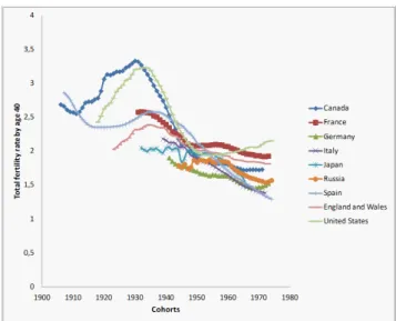
In the 20th century, growth theorists paid particular attention to interactions between, on the one hand, the production of goods, and, on the other hand, fertility behavior, that is, the production of men. When studying those inter-actions, they have mainly focused on one aspect of fertility: the number or quantum of births. From that perspective, the key stylized fact to be explained is the declining trend in fertility.1 That decline is illustrated on Figure 1, which
shows the cohort total fertility rate (hereafter, TFR) for cohorts of women aged 40 in industrialized countries. That fertility decline was explained through var-ious channels, such as the rise in the opportunity costs of children (Barro and Becker 1989), a shift from investment in children’s quantity towards children’s quality caused by lower infant mortality (Erhlich and Lui 1991, Doepke 2005, Bhattacharya and Chakraborty 2012), a rise in the return to education (Galor and Weil 2000), a rise in women’s relative wages (Galor and Weil 1996), and the rise of contraception (Bhattacharya and Chakraborty 2017, Strulik 2017).
Figure 1: Cohort total fertility rate by age 40 (source: Human Fertility Database)
Although those models cast substantial light on interactions between fertility and development, their exclusive emphasis on the quantum of births leaves aside another important aspect of fertility, which has a strong impact on economic development: the timing or tempo of births. Studying the tempo of births - and not only the quantum of births - matters for understanding long-run economic development, because of two distinct reasons.
1Note that, although the long-run trend of the TFR is decreasing, the TFR can nonetheless exhibit signi…cant short-run ‡uctuations around that trend, as shown on Figure 1.
First, theoretical papers, such as Happel et al (1984), Cigno and Ermisch (1989) and Gustafsson (2001), studied, at the microeconomic level, the mech-anisms by which the birth timing decision is related to education and labor supply decisions. A lower wage early in the career reduces the opportunity cost of an early birth, and pushes towards more early births (substitution e¤ect), but limits also the purchasing power, which pushes towards fewer early births (income e¤ect). Moreover, investing in education raises the purchasing power in the future (which pushes towards more late births), but, at the same time, raises also the opportunity cost of future children (which pushes towards fewer late births). Those strong interactions between birth timing, education and labor decisions at the temporary equilibrium motivate the study, in a dynamic model, of how development a¤ects - and is a¤ected by - birth timing.
Second, there is also strong empirical evidence supporting the existence of complex, multiple interactions between the tempo of births and various eco-nomic variables, with causal relations going in both directions. Demographic studies show that the tempo of births is strongly correlated with the education level, which a¤ects the human capital accumulation process (see Smallwood, 2002, Lappegard and Ronsen 2005, Robert-Bobée et al 2006). Moreover, sev-eral works, such as Schultz (1985), Heckman and Walker (1990) and Tasiran (1995), show that a rise in women’s wages tends to favor a postponement of births.2 There is also evidence that the wage level is a¤ected by the timing of
births (see Miller 1989, Joshi 1990, 1998, Dankmeyer 1996).
The timing of births has varied signi…cantly during the 20th century, as illustrated on Figure 2, which shows the cohort mean age at motherhood by age 40 (hereafter, MAM).3 Whereas patterns di¤er across countries, Figure 2
reveals an important stylized fact: the MAM exhibits, across cohorts, a U-shaped pattern. The MAM has been …rst decreasing for cohorts born before 1940/1950, and, then, has been increasing for later cohorts.4
The U-shaped pattern for the MAM raises several questions. A …rst question concerns the economic causes and consequences of that non-monotonic pattern. How can one explain that economic development is associated …rst with advanc-ing births, and, then, with postponadvanc-ing births? How can one relate this stylized fact with income and substitution e¤ects, and with the education decision? An-other key question concerns the relation between the dynamics of the quantum of births (Figure 1) and the tempo of births (Figure 2). Why is it the case that, at a time of strong fertility decline, cohorts tended to advance births, and, then, tended to postpone births once total fertility was stabilized?
2Those studies focused on Sweden. Similar results were shown for Japan (Ermish and Ogawa 1994), for Canada (Merrigan and Saint-Pierre 1998), and for the UK (Joshi 2002).
3The cohort mean age at motherhood by age 40 is computed for all births combined (and not only for …rst births). Consequently, this measure depends on the quantum of births (women having more children being likely to be older, on average, when giving birth to a child). Our paper focuses precisely on this relation between the tempo of births and the quantum of births.
4Note that the timing of the reversal varies across countries. For instance, in Russia, the reversal of the mean age at motherhood occurred for cohorts born in the late 1960s.
Figure 2: Cohort mean age at motherhood by age 40 (Source: Human Fertility Database)
The goal of this paper is precisely to cast some light on the relation between the quantum of births, the tempo of births, and economic development. For that purpose, we propose to adopt a Uni…ed Growth Theory approach. As pioneered by Galor (see Galor and Moav, 2002, Galor, 2010), Uni…ed Growth Theory pays a particular attention to the relation between quantitative changes (i.e. changes in numbers) and qualitative changes (i.e. changes in the form of relations between variables).5 Qualitative changes are studied by means of
regime shifts, which are achieved as the economy develops, and which cause major changes in the relations between fundamental variables. The fact, shown on Figure 2, that development was …rst associated with an advancement of births, and, then, with a postponement of births, can be regarded as a major qualitative change. Our paper aims at developing a single uni…ed framework of analysis to understand the relation between development and birth timing, and, as such, can be regarded as a contribution to Uni…ed Growth Theory.6
For that purpose, this paper develops a three-period overlapping generations (OLG) model with lifecycle fertility, that is, with two fertility periods (instead of one as usually assumed). In our model, individuals decide not only the quantum of births, but, also, how they allocate those births along their lifecycle, that is, the tempo of births. In order to study the interactions between birth timing
5Recent works in that approach include de la Croix and Licandro (2013), de la Croix and Mariani (2015), Lindner and Strulik (2015) and Strulik (2016).
6As argued by Galor (2011, p. 141), Uni…ed Growth Theory refers to a class of economic theories that "capture the entire growth process within a single uni…ed framework of analysis". Our model, which provides a single uni…ed framework to analyze the relation between fertility and development, is in line with that class of theories, even though it does not consider all facets of development, but only its relations with the quantum and the tempo of births.
and education, we also assume that individuals choose how much they invest in their education when being young, which will a¤ect their future productivity.
Anticipating our results, we show, using a general model with additively separable preferences, that there exist conditions on preferences such that, de-pending on the prevailing level of human capital, the temporary equilibrium takes three distinct forms, which correspond to three distinct regimes. In each of those regimes, a rise in human capital pushes towards fewer births. However, those regimes di¤er regarding the relation between human capital and the tim-ing of births. In the …rst regime, which prevails for low levels of human capital, individuals do not invest in education, and rises in human capital push them towards advancing births (a decline of the MAM). In the second regime, which is achieved once human capital crosses a …rst threshold, individuals start investing in education, but education remains so low that human capital accumulation still makes individuals advance births. Then, once human capital is su¢ ciently high, and reaches a second threshold, the economy enters a third regime, where human capital accumulation leads to postponing births (a rise in the MAM).
Whereas the last, modern regime (with declining TFR and births postpone-ment) was studied in the literature (see Iyigun 2000), a merit of this paper is to highlight the existence of two anterior regimes, where the decline of the TFR is associated not with the postponement of births, but with the advancement of births. In particular, the second regime, which exhibits increasing education and births advancement, has received little attention so far, but plays a key role in the transition from a traditional economy with a high TFR and a decreasing MAM to a modern economy with a low TFR and an increasing MAM.
The conditions on preferences leading to the existence of those regimes have three main aspects, which admit intuitive economic interpretation. First, those conditions guarantee that, as human capital accumulates, the substitution e¤ect dominates the income e¤ect for both early and late fertility rates (leading to a fall of TFR). Second, the conditions on preferences are such that, beyond some threshold for human capital, the level of education becomes positive and increas-ing with human capital. Third, standard assumptions on preferences imply also that the level of education tends to weaken the strength of the substitution ef-fect with respect to the income e¤ect for late births only. This latter property explains that, once education reaches a su¢ ciently high level, the tendency to advance births as human capital accumulates (which prevails for low levels of human capital) is replaced by a tendency to postpone births, leading to the U-shaped curve for the MAM.
Our dynamic lifecycle fertility model can thus rationalize both the decrease in fertility and the U-shaped pattern of the mean age at motherhood. That rationalization of the non-monotonic relation between development and birth timing is achieved by means of regime shifts as the economy develops, without having to rely on exogenous shocks. Besides this analytical …nding, we also explore the capacity of our model to replicate numerically the dynamics of the quantum and the tempo of births. Using data for 28 countries from the Human Fertility Database (cohorts 1906-1975), we show that our model can, with some degree of approximation, …t the patterns of the TFR and the MAM.
Our paper is related to several branches of the literature. First of all, it com-plements microeconomic studies of birth timing, such as Happel et al (1984), Cigno and Ermisch (1989) and Gustafsson (2001), which examine birth tim-ing decisions in a static setttim-ing, whereas we propose to draw the corollaries of those decisions for long-run dynamics. Second, we also complement the litera-ture focusing on the relation between birth timing and long-run development. In a pioneer paper, Iyigun (2000) showed, by means of a 3-period OLG model with two fertility periods, that human capital accumulation leads to the post-ponement of births. While Iyigun’s paper rationalizes the increasing part of the U-shaped curve for the MAM, our paper provides a rationalization for the entire U-shaped curve, including its decreasing segment.7 Our paper
comple-ments also other papers, such as, in continuous time, d’Albis et al (2010), and, in discrete time, Momota and Horii (2013) and Pestieau and Ponthiere (2014, 2015). Those papers examined the relation between, on the one hand, physi-cal capital accumulation, and, on the other hand, the quantum and tempo of births.8 Whereas those papers paid attention to the existence and stability of a stationary equilibrium under several fertility periods, our paper adopts, on the contrary, a Uni…ed Growth Theory approach, where regime shifts are used to rationalize the non-monotonic pattern exhibited by the tempo of births.
The rest of the paper is organized as follows. Section 2 has a closer look at the data, and examines the statistical signi…cance and the robustness of the stylized facts concerning the quantum and the tempo of births, as well as the relation between fertility behavior and education. The model is presented in Section 3. Section 4 characterizes the temporary equilibrium, and examines the distinct regimes. Long-run dynamics is studied in Section 5. An analytical example is developed in Section 6. Section 7 illustrates our …ndings numerically, by focusing on cohorts of the Human Fertility Database. Section 8 concludes.
2
Stylized facts
Before considering how a theory of the quantum and the tempo of births can be developed to rationalize the two stylized facts mentioned in Section 1 (the declining long-run trend in cohort TFR and the U-shaped trend for cohort MAM), it is useful to have a closer look at the data, in order to examine the statistical signi…cance and robustness of those stylized facts, and, also, in order to explore the relation between those stylized facts and education data.
Regarding the issue of statistical signi…cance and robustness, we run sim-ple statistical regressions using data from the Human Fertility Database. The data provides measures of cohort fertility by age 40 (TFR) and cohort mean
7Another related paper is Sommer (2016), which studies the relation between the quantum and the tempo of births under risk (in earnings and fertility). More recently, de la Croix and Pommeret (2017) study the optimal timing of births under fertility risks. Unlike those papers, our study involves no risk, but adopts a Uni…ed Growth Theory approach with multiple regimes.
8The interactions between the quantum of births and physical capital accumulation are studied under more general preferences in Momota (2016).
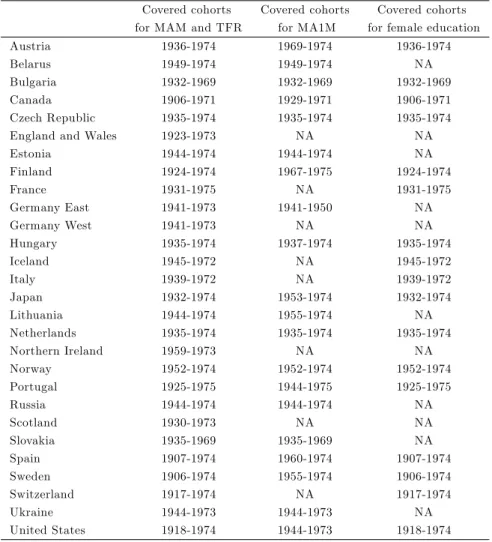
age at childbirth by age 40 (MAM) for 28 countries, for cohorts 1906 to 1975 (unbalanced panel). Table A1 in the Appendix provides an overview of covered countries and cohorts for the variables used in this section. Regressions are all run with country-…xed e¤ects. These models include country-speci…c dummies which implicitly control for country-speci…c variables that are constant over time. Our …xed-e¤ects models therefore focus on within-country variations.
The data con…rms, …rst of all, the existence of a long-run declining trend in cohort fertility at age 40 (cohort TFR).9 Concerning the tempo of births, our
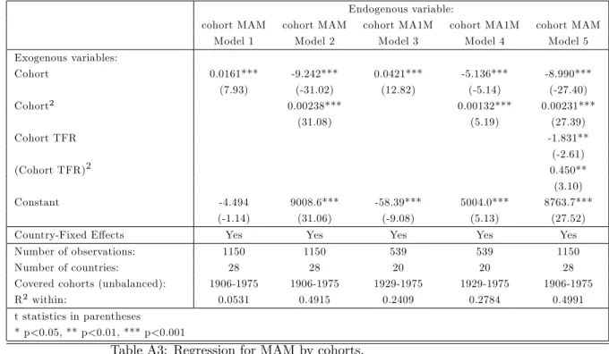
regressions con…rm the existence of a statistically signi…cant U-shaped relation between the birth year of cohort and the cohort MAM.10 The estimated
U-shaped relation is shown on Figure 3, with a 95 % con…dence interval.
Figure 3: MAM by age 40 by cohorts (source Human Fertility Database).
The estimated U-shaped pattern is somewhat ‡atter than the one that is actually observed for most countries. This is partly due to a di¤erence in the timing of the reversal. Some countries, such as France, exhibit a reversal for co-horts born in the 1940s, whereas in other countries, such as Russia, the reversal took place for cohorts born only in the 1960s. In addition, the estimated curve is ‡attened by the fact some countries join the panel later than others. It is likely that for these countries, we do not observe the full declining branch and/or the
9See, in the Appendix, Table A2 for the regression and Figure A1 for the graphical repre-sentation of the evolution of cohort TFR across cohorts. For most countries, the overall trend exhibited by the TFR is a decline over the observed cohorts. Two major exceptions are the United States and Canada, for which cohort TFR increases for cohorts 1910 to 1930.
1 0See Table A3 in the Appendix. Note that a cubic speci…cation has also been tested for the cohort MAM, but was found to be non-signi…cant (results available on request).
full re-increasing branch. However, despite the fact that the estimated U-shaped curve is ‡atter than the one for each country, it remains nonetheless statisti-cally signi…cant. Thus the stylized fact of a U-shaped cohort MAM is a robust empirical fact, which is not speci…c to only some of the observed countries.11
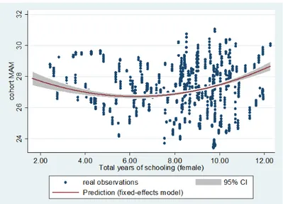
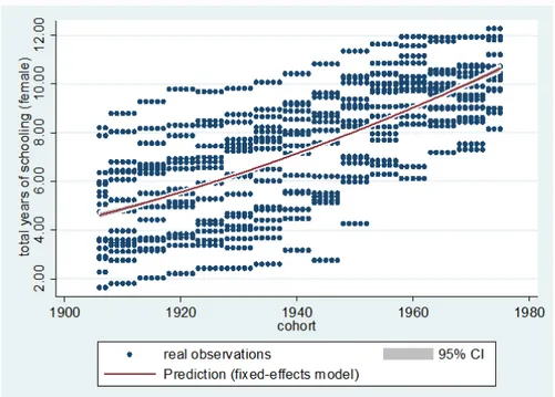
Given that education will play a key role in our theory of the quantum and the tempo of births, it is also worth considering data on education, and their relation with the TFR and the MAM. As cohort data on education is not available for most cohorts of interest, we use, as a second-best option, periodic data and assign the period measures to our cohorts 1906-1975. We use estimates on education attainment for the female population aged 15-24, which come from the Lee and Lee (2016) Long-Run Education Dataset, and cover years 1870 to 2010 (5-year intervals). In order to assign the periodic observations of the average years of total schooling (primary, secondary and tertiary) of a female population aged 15-24 to our birth cohorts of 1906 to 1974, we allow a 20-year delay between the periodic observations of education and our cohorts.12 As shown in the Appendix, female educational attainment has been growing over the cohorts born during the 20th century for all countries.13
Figure 4: Cohort MAM by education (sources: Human Fertility Database and Lee-Lee Long-Run Education Dataset).
1 1Note that, as discussed in the Appendix, the estimated path for the mean age at …rst motherhood (MA1M) over cohorts exhibits also a U-shaped pattern, but the declining branch is smaller than the rising branch, which is most likely due to the fact that observations of MA1M are not available for cohorts born earlier than 1929 for the majority of countries.
1 2See the Appendix for the extrapolation of cohort educational attainments from period educational attainments observations.
1 3Figure A2 in the Appendix shows the countries’average years of female schooling assigned to the cohorts 1906-1974 as well as the estimated within-country path.
When relating education attainment with fertility behavior, a …rst observa-tion is that, for the cohorts under study, there has been both a decline in the quantum of births, as well as a rise in education over cohorts (Figures A1 and A2 in the Appendix). Regarding the relation between cohort education and the tempo of births, one would, at …rst glance, expect that the rise in education is associated with a postponement of births. However, as shown in Figure 4, which contrasts the country-observations to the estimated within-country path, the relation between cohort education (average years of schooling: primary, sec-ondary and tertiary) and the cohort MAM is non monotonous, and exhibits a U-shaped form. This U-shaped relation between education and MAM is robust to the de…nition of the education variable, and remains statistically signi…cant even when education is restricted to only secondary and tertiary education.14
Figure 4, which plots real country observations against the regression result of Model 1 in Table A4 in the Appendix, can be interpreted as follows. Con-trary to what one may expect at …rst glance, the relation between education and the tempo of births is not always increasing for the observed cohorts. Ac-tually, there exists a threshold level in education such that, for education levels below the threshold, an increase in education leads to a reduction in the MAM (advancement of births), whereas, for education levels above the threshold, an increase in education leads to a rise in the MAM (postponement of births).
The goal of the next sections is to develop a simple theoretical model ratio-nalizing the declining trend in the TFR, the U-shaped pattern for the MAM, as well as the U-shaped relation between education and the MAM.
3
The model
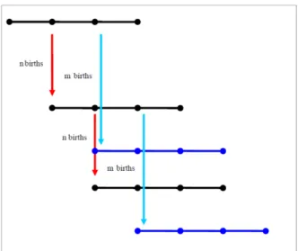
Let us consider a three-period OLG model with lifecycle fertility. Time goes from 0 to +1. Each period has a unitary length. Period 1 is childhood, during which the child is raised by the parent, and does not make any decision. Period 2 is early adulthood, during which individuals work, consume, have ntchildren
and invest in education. Period 3 is mature adulthood, during which individuals work, consume, and can complete their fertility by having mt+1children. Figure
5 shows the formal structure of the model.
Figure 5: The lifecycle fertility model.
Production Production involves labor and human capital. The output of an agent at time t, denoted by yt, is equal to:
yt= ht`t (1)
where htis the human capital of the agent at time t, while `tis the labor time.
Human capital accumulation When becoming a young adult at time t, each agent is endowed with a human capital level ht> 0.15 htdetermines the
marginal productivity of labor when being a young adult.
The young adult can invest in education, in such a way as to increase his human capital stock at the next period. Human capital accumulates according to the law:
ht+1= (v + et) ht (2)
where etdenotes the level of e¤ort/investment in education, while v is an
mulation parameter, which determines the rate at which human capital accu-mulates in the absence of education (i.e. when et= 0).
Throughout this paper, we will suppose that v > 1, that is, that even in the absence of education, individuals can become more productive over time. Human skills can improve despite the absence of education, because either of a
1 5This uniformity of endowments across all individuals born at the same point in time (independently from the age of their parent) allows us to keep a representative agent structure, unlike in Pestieau and Ponthiere (2016), where early and late children, who di¤er in terms of time constraints, are studied as two distinct populations.
standard learning by doing mechanism, or of an exogenous technological progress raising the productivity of labor.16
We assume here that education takes the form of a monetary, non-temporal, physical e¤ort, which is a source of disutility. This non-standard formulation allows us to provide an analytically tractable framework by reducing the number of possible regimes (and sequences of regimes) that can emerge as human capital accumulates (see infra).17
Budget constraints It is assumed that raising a child has a time cost q 2 ]0; 1[. That cost is supposed to be the same for early and late children. Assuming that there is no saving, so that each agent consumes what he produces at each period of life, the budget constraint at early adulthood is:
ct= ht(1 qnt) (3)
where ct denotes consumption at early adulthood for a young adult at time t.
The budget constraint at mature adulthood is:
dt+1= ht+1(1 qmt+1) (4)
where dt+1 denotes consumption at mature adulthood for a mature adult at
time t + 1.
Assuming that there is no possibility for individuals to save or to borrow resources is in line with Uni…ed Growth Theory (Galor 2011). Whereas that as-sumption simpli…es the picture, it should be stressed that education and savings are quite redundant in the present context, since these are two ways to transfer resources over time. As far as fertility choices are concerned, education and savings are also redundant: by increasing the hourly wage in period 3, human capital and physical capital accumulations are two ways to increase the future purchasing power of individuals (which push, through an income e¤ect, towards more late births), and, also, two ways to increase the opportunity cost of having late births (which push, through a substitution e¤ect, towards fewer late births). Given this redundancy, and the necessity to keep the model parsimonious, this framework will abstract from savings choices.18
1 6The assumption v > 0 is widespread in the literature (see de la Croix and Doepke 2003 and Moav 2005). Assuming v > 1 is stronger but that assumption is close to what Kremer (1993) assumed in his seminal paper, where the variable re‡ecting knowledge or labor productivity grows at a positive rate as long as the population size is positive.
1 7Since the marginal return of education is ht, the marginal utility gain from investing in education at et = 0 is increasing in ht. Our assumption of a physical education e¤ort, by implying that the marginal disutility of education is constant with ht, guarantees the existence of a single threshold for ht below which et = 0and above which et > 0(see infra ). If, on the contrary, education e¤ort were time, the marginal disutility of investing in education at et = 0would be increasing in ht, so that there could be several thresholds for ht de…ning a succession of regimes with zero or positive education. Our assumption prevents that this counterintuitive case appears.
1 8The reasons why we focus on education choices rather than on savings choices are twofold. First, demographic studies emphasized the key role played by education choices for the timing
Preferences Individuals derive utility from consumption and from hav-ing children. They also derive disutility from investhav-ing e¤orts in education. Individuals are endowed with time-additive preferences having the form:19
U (ct; nt; et) + V (dt+1; mt+1) (5)
where U ( ) and V ( ) are additively separable in their components, increasing and strictly concave with respect to (ct; nt; dt+1; mt+1). Moreover, we assume
that U ( ) is strictly decreasing and strictly convex with respect to et.
With respect to fertility, an important feature of that utility function is that it exhibits limited substitutability between early births and late births. The main justi…cation for this feature is that, in the same way as there is no perfect substitutability for the allocation of consumption across time periods, there is no perfect substitutability for the allocation of births across time periods.
Regarding preferences over early children and late children, it should be stressed that our utility function treats all children as sources of temporal wel-fare at the period of their birth. Alternatively, one may want to treat children as durable goods, and make third-period welfare depend not only on late chil-dren, but, also, on early children. Whereas treating children as durable goods is a potentially fruitful approach, we prefer here to rely on a more standard formulation, to avoid that our results are driven by a too asymmetric treatment of early children and late children at the level of parental preferences.20
4
The temporary equilibrium
At the beginning of early adulthood, individuals choose consumptions ct and
dt+1, the education e¤ort et, the number of early children nt, and the number of
late children mt+1, in such a way as to maximize their lifetime welfare, subject
to budget constraints.
Throughout this paper, we will, without loss of generality, look at a solution that is interior for (ct; nt; dt+1; mt+1). However, we will allow the education
e¤ort etto be a corner solution.
The problem faced by young adults can be written as:
max (ct;nt;et;dt+1;mt+1) U (ct; nt; et) + V (dt+1; mt+1) ; s:t: ct= ht(1 qnt) ; dt+1= ht( + et) (1 qmt+1) ; et 0:
of births (see Smallwood 2002, Lappegard and Ronsen 2005 and Robert-Bobée et al 2006). This makes the education variable more relevant than savings for the study of births timing. Second, works by Momota and Horii (2013) and Pestieau and Ponthiere (2014, 2015) examined the relation between physical capital accumulation and the timing of births.
1 9Being time-additive, those preferences guarantee that fertility choices are time consistent. 2 0Note also that, in our representation of preferences, it is still possible to account indirectly for the longer period of coexistence of parents with early children than with late children, simply by assigning a larger weight to early births than to late births.
The …rst-order conditions (FOCs) for, respectively, optimal interior levels of early fertility nt, education etand late fertility mt+1, are:
Ucthtq + Unt = 0; (6)
Uet+ Vdt+1ht(1 qmt+1) + t = 0; (7) Vdt+1ht( + et) q + Vmt+1 = 0; (8)
where t is the multiplier associated to the inequality constraint on et. The
complementary slackness condition is therefore:
et t= 0: (9)
When considering those FOCs, we see that the prevailing stock of human capital htconstitutes a major determinant of individual choices in terms of
fer-tility (number and timing of births). A rise in ht leads to both a rise in the
opportunity cost of having children (substitution e¤ect), which pushes towards fewer births, and to a rise of the purchasing power of the individual (income e¤ect), leading to more births. The strength of those various income and sub-stitution e¤ects, by a¤ecting the early and late fertility rates nt and mt+1,
determines the reactivity of the TFR (equal to nt+ mt+1) and of the MAM
(equal to nt+2mt+1
nt+mt+1 ) to variations in human capital ht.
Since ht is the unique latent variable in our model, studying the dynamics
of the TFR and the MAM is equivalent to examining how these variables react to variations in ht. In the rest of this section, we derive su¢ cient conditions on
preferences for the existence of the following three regimes, whose occurrence depends on the prevailing level of human capital ht:
1. Regime I: et= 0 and the TFR and the MAM decrease in ht;
2. Regime II: et> 0 and the TFR and the MAM decrease in ht;
3. Regime III: et> 0, the TFR decreases in htand the MAM increases with
ht.
In order to derive conditions on preferences that are su¢ cient for the exis-tence of those three regimes, this section proceeds in four successive steps, each step of the proof being associated with a lemma:
Lemma 1 states conditions under which ntand mt+1are decreasing in ht
and MAM decreases with htwhen et= 0.
Lemma 2 states conditions under which ntand mt+1are decreasing in ht
and etincreases with ht when et> 0.
Lemma 3 states conditions under which there exists a threshold h below which et= 0 and above which et> 0.
Lemma 4 states conditions under which there exists a second threshold ~
h > h below which the MAM decreases with htand above which the MAM
Taken together, the conditions on preferences stated in those four lemmas su¢ ce to prove the existence of Regimes I, II and III. Given that our general framework does not rely on particular functional forms for U ( ) and V ( ), those conditions are quite general, and these point to key features of preferences that lead to rationalizing both the decline of TFR and the U-shaped MAM. Another advantage of our general model lies in the fact that it allows us to provide eco-nomic interpretations of those conditions on preferences in terms of income and substitution e¤ects for early and late births. By doing so, our general framework contributes to generalize the microeconomic analysis of fertility choices, which focussed only on the microeconomic determinants of the quantum of births, without examining the determinants of the tempo of births.21
Regarding notations, we will, throughout this section, abstract from time indexes, as they are not necessary here: the solution of the individual’s program is a set of functions of h that we denote as follows: n , e and m . Analyzing the responses of those variables with respect to h is equivalent to analyzing their behavior with respect to time, as h is the only latent variable in the model.
For that purpose, let us de…ne the elasticities of early fertility n and late fertility m , computed at the optimum, with respect to h, as:
"nh:= @n @h h n and "mh:= @m @h h m : (10)
Moreover, it is convenient to de…ne the following elasticities:
"c := Uccc Uc , "n:= Unnn Un , "e:= Ueee Ue , "d:= Vddd Vd , "m:= Vmmm Vm ; (11) which are evaluated at the optimum and are all positive.
Let us …rst assume the existence of Regime I (i.e. e = 0), and consider the reactions of n and m to human capital conditionally on being in Regime I.22
Lemma 1 Suppose that e = 0. The optimal responses of early and late fertility rates to human capital satisfy:
"nh = 1 "c "c1 qnqn + "n
and "mh= 1 "d "d1 qmqm + "m
: (12)
Thus, the TFR decreases with h if "c < 1 and "d < 1. Moreover, the MAM is decreasing with h if:
1 "c "c1 qnqn + "n <
1 "d
"d1 qmqm + "m: (13)
2 1One drawback is that those general conditions may look quite abstract, so that it is not easy to see how restrictive those conditions are. However, we will show, when examining an analytical example in Section 6, that those general conditions have a simple counterpart once particular functional forms are imposed on U ( ) and V ( ).
Proof. See the Appendix.
As stated above, a rise in the human capital stock implies a rise in the opportunity cost of having children, which pushes towards fewer births, as well as a rise in the purchasing power of individuals, which favors more births. The conditions "c < 1 and "d< 1 stated in Lemma 1 imply that, for both early births and late births, the substitution e¤ect dominates the income e¤ect, implying that n and m are decreasing with human capital. As a consequence, those conditions on preferences imply that, as human capital accumulates, the TFR, equal to n + m , declines. This result is in line with the fertility transition.
Regarding the timing of births, whether the MAM is increasing or decreasing in human capital depends on the relative strengths of the responses of n and m to variations of human capital. We have that the MAM is decreasing in human capital (i.e. an advancement of births) when the rate at which n falls is smaller, in absolute value, than the rate at which m falls. Expression (13) states the condition on preferences under which, in the absence of education, the rate at which the early fertility rate falls when human capital accumulates is, in absolute value, lower than the rate at which the late fertility rate falls, leading to the advancement of births.23
Let us now assume the existence of regimes characterized by a non-binding investment in education (i.e. e > 0), and characterize the responses of fertility rates and education to human capital in those regimes.24
Lemma 2 Suppose that e > 0. The optimal responses of early fertility to human capital is the same as in (12), and thus n decreases with h if "c < 1. The optimal response of late fertility to human capital satis…es:
"mh= 1 "d qm 1 qm "d+ "m + 1 qmqm + "m (1 "d) ("e +e e 1) : (14)
Moreover, m decreases with h and e increases with h if "d< 1 and:
"e + e e < "d
(1 "d)2
"d+ "m1 qmqm : (15)
Proof. See the Appendix.
Given our assumption that the cost of education is a utility cost, early fer-tility n does not depend on education. As a consequence, the response of early fertility to variations in human capital is the same expression as in Regime I (when education equals zero), implying that the condition guaranteeing that n is decreasing in human capital is the same as in Lemma 1 (i.e. "c < 1).
On the contrary, the late fertility rate m is impacted by education, and the response of late fertility to human capital "mh is also impacted, in a way that
2 3That condition, expressed in terms of elasticities, may seem quite abstract, so that it is di¢ cult, at …rst glance, to see how restrictive it is. We show in Section 6 that this condition takes a simple form under standard functional forms for U ( ) and V ( ).
depends on the level of education, and on how education a¤ects the relative sizes of the substitution and income e¤ects. When the preferences satisfy "d< 1 and (15), it is still the case that the substitution e¤ect dominates the income e¤ect, and that m decreases with h. Those conditions also guarantee that education is increasing with human capital, in line with empirical evidence.
We now turn to the existence of Regime I.
Lemma 3 There exists a unique threshold h > 0 such that e = 0 for all h h and e > 0 for all h > h if:
lim
d!0Vdd < elim!0Ue< limd!+1Vdd: (16)
and if conditions "d< 1 and (15) are satis…ed.
Proof. See the Appendix.
Lemma 3 states conditions on preferences that are su¢ cient for the existence of a single threshold in human capital h > 0 such that for any level of human capital below h, education is equal to zero, whereas for any level of h above h, education is strictly positive. The conditions on preferences include boundary conditions on utility functions, plus some conditions guaranteeing that education increases with human capital (which imply the uniqueness of the threshold h).
The reason why e = 0 when h < h lies in the fact that the marginal utility gain from investing in education is, given the low human capital stock, too low with respect to the marginal disutility of education e¤orts, which makes investment in education not worthy. However, once h > h, it becomes desirable to invest in education, leading to e > 0. Thus Lemma 3 shows that the economy is in Regime I if h h, and does not lie in Regime I when h > h.
Finally, Lemma 4 provides conditions on preferences under which there exists a unique level of human capital below which the MAM is decreasing in human capital, and beyond which the MAM is increasing with human capital, implying thus the existence of Regime III.
Lemma 4 There exists a threshold ~h > h such that the MAM is decreasing with h for h ~h and is increasing with h for h > ~h if condition (13) is satis…ed, if
lim
e!+1
Uee
Ue
( + e) = 1; (17)
and if limd!+1Vdd is not too large. Moreover, ~h is unique if:
@ (j"nhj j"mhj)
@h h=~h> 0: (18)
Proof. See the Appendix.
Condition (17) guarantees that, when education is su¢ ciently large, it is necessarily the case that the elasticity of early births to human capital exceeds, in absolute value, the elasticity of late births to human capital, so that j"nhj >
j"mhj. Jointly with the condition on the limd!+1Vdd, it implies that there
exists at least one threshold ~h at which j"nhj = j"mhj, so that the derivative of the MAM with respect to h equals 0. The uniqueness of that threshold is guaranteed by condition (18). The intuition behind that condition goes as follows. We know, under the conditions of Lemma 1, that the MAM is decreasing with h for a low h, that is, that j"nhj < j"mhj. We also know that, when h tends
to +1, the MAM is increasing with h, that is, j"nhj > j"mhj. Hence a necessary
and su¢ cient condition for uniqueness of the threshold ~h at which j"nhj = j"mhj is that the derivative of (j"nhj j"mhj) is positive at any such ~h. This condition
is given by (18).
In economic terms, the conditions in Lemma 4 can be interpreted as follows. From Lemma 1, we know that, under our conditions on preferences, the MAM is decreasing with human capital when education equals zero. Moreover, from Lemma 2, our conditions on preferences imply that education, once positive, is increasing with h. The conditions stated in Lemma 4 can be interpreted as conditions that imply that there exists a unique threshold in terms of education, below which the MAM is decreasing with h (i.e. advancement of births), and above which the MAM becomes increasing with h (i.e. postponement of births). This reversal of the sign of the impact of human capital on the MAM suggests that, under our assumptions, education tends to weaken the relative strength of the substitution e¤ect with respect to the income e¤ect for late births, but not for early births (since the response of early births to h is not a¤ected by the level of education).
The conditions stated in Lemma 4 guarantee that Regime III prevails when h > ~h > h. Given that we know, from Lemma 3, that Regime I prevails when h < h < ~h, we can deduce from Lemmas 3 and 4 that there must exist an intermediate interval for human capital (h; ~h] where Regime II prevails. Indeed, in that interval, we know from Lemma 3 that education is strictly positive, and from Lemma 4 that the MAM is decreasing with h. These are the two features of Regime II. Our results are summarized in Proposition 1.
Proposition 1 Let us assume that "c < 1 and "d< 1 and that conditions (13), (15), (16), (17) and (18) are satis…ed. Then there exist three regimes. The human capital in Regime I is lower than that of Regime II, which is lower than that of Regime III. The three regimes are characterized as follows:
In Regime I (h h), there is no education and the TFR and the MAM decrease with human capital.
In Regime II (h < h ~h), education is positive and increases with human capital, while the TFR and the MAM decrease with human capital.
In Regime III (~h h), education is positive and increases with human capital, the TFR decreases with human capital, while the MAM increases with human capital.
Proposition 1 states conditions on preferences such that, depending on the prevailing level of the human capital stock, the economy is either in Regime I, or in Regime II, or in Regime III. Those conditions, which are presented in the previous lemmas, have three main aspects, which admit intuitive economic interpretation. First, those conditions guarantee that, as human capital accu-mulates, the substitution e¤ect dominates the income e¤ect for both early and late fertility rates (leading to a fall of the TFR). Second, the conditions are such that the level of education becomes positive beyond some threshold of human capital, and increasing with human capital. Third, our assumptions on prefer-ences imply also that the level of education tends to weaken the strength of the substitution e¤ect with respect to the income e¤ect for late births only (and not for early births). This explains that, once education reaches a su¢ ciently high level, the tendency to advance births as human capital accumulates (which prevails for low levels of human capital) is replaced by a tendency to postpone births, leading to the U-shaped curve for the MAM.
Each of the three regimes described in Proposition 1 can be regarded as a distinct stage of development, with particular relations between human capital, the quantum of births (i.e. the TFR) and the tempo of births (i.e. the MAM).
Under Regime I, the response of early fertility to human capital accumula-tion is, in absolute value, lower than the one of late fertility. Thus, the MAM decreases with human capital, leading to an advancement of births. In Regime II, where education is positive, the response of late fertility is still higher than the one of early fertility, so that the MAM continues to decrease. But when education reaches a su¢ ciently high level, the economy enters Regime III, and the response of late fertility becomes lower, in absolute value, than the one of early fertility, so that the MAM starts increasing with human capital, leading to a postponement of births.
Thus, when comparing Regime III with Regimes I and II, there is an im-portant qualitative change. Whereas the rise in income used to push towards advancing births in Regimes I and II, this is no longer the case in Regime III, where the rise in income pushes towards postponing births. This third regime coincides with what could be called the modern regime, where the decline in fertility is associated with births postponement.
5
Economic and demographic dynamics
Having shown that the temporary equilibrium can take three distinct forms, depending on the prevailing level of human capital, let us now describe how the economy evolves over time, that is, how the economy shifts from one regime to another as human capital accumulates.
For that purpose, let us assume that the economy starts at an initial human capital level h0 < h. Let us also make all assumptions on preferences made in
Proposition 1. Thus, using Proposition 1, the economy lies initially in Regime I. Given v > 1, human capital grows in Regime I, so that it will, sooner or later, cross the threshold h, leading the economy to Regime II, where education
becomes positive. Note that, in Regime II, the growth rate of human capital is positively correlated with education, which is itself increasing with human capital. Given those relations, the growth rate of human capital is larger in Regime II than in Regime I, and the human capital stock will, sooner or later, cross the second threshold, i.e. ~h > h, which coincides with entry in Regime III. Hence, starting from an initial human capital h0 < h, the economy will move
from Regime I to II and from Regime II to III, and then stay in Regime III. This transition from Regime I to Regime II, and from Regime II to Regime III has some consequences in demographic terms. From Proposition 1, we can see that this implies that the TFR exhibits a declining trend, which is in line with the fertility transition. Moreover, we also know from Proposition 1 that the shift from Regimes I and II to Regime III leads to a reversal of the relationship between human capital and the MAM. Whereas economic development was associated with the advancement of births (i.e. a decreasing MAM) in Regimes I and II, this is not the case in Regime III, where development leads to postponing births (i.e. an increasing MAM). Thus, as the economy develops, the MAM exhibits the U-shaped curve, in line with the stylized fact identi…ed above.
Proposition 2 summarizes our results concerning long-run dynamics.
Proposition 2 Assume an initial human capital h0 < h. Assume also the
conditions made in Proposition 1.
The economy is initially in Regime I, and tends, as human capital accu-mulates, to shift from Regime I to Regime II, and, then, from Regime II to Regime III.
The growth rate of human capital is lower in Regime I than in Regime II, and lower in Regime II and in Regime III.
Over time, the TFR and MAM variables exhibit the following patterns:
–The TFR exhibits a decreasing pattern; –The MAM exhibits a U-shaped pattern.
Proof. Proposition 2 is a corollary of the accumulation law ht+1 = (v + et)ht
and of Proposition 1.
Proposition 2 states that our model can rationalize the observed patterns for the quantum and the tempo of births. That rationalization of the patterns for the TFR and the MAM does not rely on any external, exogenous shock. In line with Uni…ed Growth Theory (Galor 2011), the patterns for the TFR and the MAM are induced by the dynamics of a latent variable (here human capital). As that latent variable crosses some thresholds, the economy enters into di¤erent regimes, which can be regarded as distinct stages of development, characterized by di¤erent relations between economic and demographic variables.
Our rationalization of the U-shaped pattern for MAM is particularly in line with Uni…ed Growth Theory, since there is here a qualitative change, a reversal of the relation between development and the timing of births: below some level
of development, income rises push towards advancing births, whereas beyond some level of development, income rises push towards postponing births. That qualitative change is, in our model, rationalized by a shift from Regime II to Regime III as human capital accumulates.
Note that the ability of our model to rationalize the observed patterns for the TFR and the MAM relies on some conditions on preferences (see Proposition 1). Not all kinds of preferences are compatible with a decline in TFR and a U-shaped curve for MAM. Those trends can be rationalized when preferences are such that the substitution e¤ect dominates the income e¤ect for the two fertility rates (implying a decline in the TFR), and when the emergence of education weakens the strength of the substitution e¤ect relative to the income e¤ect for late births (but not for early births), implying that the rate at which late fertility declines when human capital accumulates becomes, for a su¢ ciently high level of education, lower than the rate at which early fertility reacts.
Given the general forms for U ( ) and V ( ), the conditions stated in Proposi-tion 1 are not easy to interpret, since these concern elasticities that are de…ned in terms of the variables prevailing at the temporary equilibrium. Hence it is not simple to see whether these conditions are satis…ed under standard functional forms for U ( ) and V ( ). In order to answer that question, the next section develops an analytical example based on speci…c forms for U ( ) and V ( ). This example will illustrate the scope of parametric restrictions on utility functions that can rationalize the declining TFR and the U-shaped pattern for MAM.
6
An analytical example
This section develops an analytical example of the general model presented in the previous sections. The goal of that example is not only to examine whether standard functional forms for U ( ) and V ( ) can satisfy the conditions stated in Proposition 1, but, also, to provide explicit solutions for the patterns of all variables, including the TFR and the MAM.
Preferences Let us now impose the following functional forms for the utility function:
U (ct; nt; et) : = log (ct+ ) log (et+ ) + log(nt) (19)
V (dt+1; mt+1) : = log(dt+1+ ") + log(mt+1) (20)
where > 0, > 0, > 0, > 0, > 0, " > 0, > 0 and > 0 are preference parameters. (resp. ) captures the weight assigned to consumption early (resp. late) in life. captures the disutility of education e¤orts. (resp. ) captures the taste for early (resp. late) fertility. The parameters , and " allow us to have a su¢ ciently general structure for preferences.
Temporary equilibrium Substituting for the budget constraints, the problem of the individual can be written as follows:
max
et;nt;mt+1
log (ht(1 ntq) + ) log (et+ )
+ log((v + et)ht(1 mt+1q) + ") + log(nt) + log(mt+1)
The FOCs for, respectively, optimal interior levels of early fertility nt,
edu-cation et and late fertility mt+1, are:
htq ht(1 ntq) + = nt (21) (et+ ) = ht(1 mt+1q) (v + et)ht(1 mt+1q) + " (22) (v + et)htq (v + et)ht(1 mt+1q) + " = mt+1 (23)
The …rst FOC, which characterizes the optimal early fertility level, equalizes the marginal utility gain from early fertility (RHS) with the marginal utility loss from early fertility (LHS). Note that, since > 0, the marginal utility loss of early births depends on the prevailing level of human capital. This would not be the case under = 0, since in that case the income and substitution e¤ects would cancel each other, making early fertility independent of human capital.
The second FOC states that the optimal education equalizes the marginal disutility of education e¤ort (LHS) and the marginal utility gain from extra consumption at mature adulthood thanks to education (RHS). Under " = 0, the optimal education would be independent from late fertility (and from ht).
Finally, the third FOC characterizes the optimal late fertility level. It equal-izes the marginal utility gain from late births (RHS) with the marginal utility loss from late births (LHS). Under " = 0, the marginal utility loss from late births would be invariant to human capital, which would make mt+1
indepen-dent from ht. On the contrary, under " > 0, the LHS depends on the human
capital level, which a¤ects both the purchasing power at mature adulthood and the opportunity cost of late births.
Whereas the 3 FOCs characterize a temporary equilibrium with interior levels for early fertility nt, education etand late fertility mt+1, such an interior
temporary equilibrium is not necessarily reached, depending on the level of human capital at time t.
Proposition 3 states conditions on the structural parameters under which the conditions stated in Lemmas 1 to 4 are valid, so that Proposition 1 holds and the economy exhibits the three regimes studied in the previous sections.
Proposition 3 De…ne h v("( v+ v)), (ht) [ht + ']2+4ht!v ( v ) (ht
h), ' " ( + ) and e(ht)
[ht +']+p2 (ht)
The utility function log (ct+ ) log (et+ )+ log (nt)+ log (dt+1+ ")+
log (mt+1) satis…es the conditions stated in Lemmas 1 to 4 i¤ the
para-meters satisfy:
" > v and > v ; ht 0(ht) > 2 (ht) 2'2
p (ht);
> v and is not too high
as well as: ~ h + 2 + h e00(~h)~h + e0(~h)i v + e(~h) ~h e0(~h) 2 1 " h v + e(~h)i2 v + e(~h) ~h + " > ~ h + e0(~h)~h + v + e(~h) v + e(~h) ~h + "
where ~h is the solution to: e(ht) + (ht+ ) e0(ht) ="(v + e(ht))2 v.
The three regimes can be characterized as follows:
–In Regime I (ht h), et= 0; nt= ht(hq( + )t+ ) ; mt+1= vh(vhtq( + )t+") , as well as @T F Rt @ht < 0 and @M AMt @ht < 0. –In Regime II (h < ht ~h), et = e(ht) > 0; nt= ht(hq( + )t+ ); mt+1 = ((v+e(ht))ht+") (v+e(ht))htq( + ), as well as @T F Rt @ht < 0 and @M AMt @ht < 0.
–In Regime III (~h < ht), et = e(ht) > 0; nt = ht(hq( + )t+ ); mt+1 = ((v+e(ht))ht+") (v+e(ht))htq( + ), as well as @T F Rt @ht < 0 and @M AMt @ht > 0: Proof. See the Appendix.
Proposition 3 states that, under the particular functional forms for U ( ) and V ( ), there exist conditions on the structural parameters of our economy such that the conditions stated in Lemmas 1 to 4 are satis…ed, so that Proposition 1 holds. As a consequence of Proposition 1, the economy exhibits, under those conditions, the three regimes studied in the previous sections: Regime I where education equals zero, and where both the TFR and the MAM decrease when human capital accumulates; Regime II, where education is positive and increas-ing in ht, but where the TFR and the MAM are still decreasing in ht; and,
…nally, Regime III, where education is still increasing in ht, and where the TFR
is decreasing in ht, whereas the MAM is increasing in ht.
Long-run dynamics The development process follows the same pattern as in Section 5. Assuming an initial human capital h0< h, as well as h0> ,
"
v (to guarantee non-negative consumptions at t = 0), the economy lies initially
in Regime I, and, given v > 1, human capital will grow and will sooner or later reach the threshold h, and thus enter Regime II. Given that education becomes positive in Regime II, this reinforces the accumulation of human capital, which will at one point cross the second threshold ~h, implying entry into Regime III.
The monotonicity of education in human capital guarantees that the economy will then remain in Regime III.
Regarding demographic variables, the economy exhibits all along a decreas-ing TFR, while the MAM, which is decreasdecreas-ing in htin Regimes I and II, becomes
increasing in htin Regime III, and, hence, exhibits a U-shaped form.
While those results are already obtained in the general model, an important contribution of this analytical example is that this allows us to compute the long-run levels of the TFR and the MAM. These are obtained by taking the limit of nt and mt+1when human capital tends to in…nity.25 We obtain:
lim ht!1 nt= q ( + ) > 0 and hlimt!1 mt+1= q ( + ) > 0
Thus the TFR and MAM converge asymptotically towards, respectively:
T F R1 =
q ( + )+q ( + )
M AM1 = ( + ) + 2 ( + )
( + ) + ( + )
Thus, whereas human capital keeps on increasing over time without limit, the quantum and the tempo of births tend to stabilize over time. The asymptotic TFR depends on the preference parameters , , and , as well as on the time cost of children q. Regarding the timing of births, the asymptotic MAM does not depend on the time cost of children (which is the same for early and late births), but only depends on preference parameters , , and .
7
Numerical illustration
The previous Sections show that our model can, qualitatively, explain or ratio-nalize the global patterns exhibited by the quantum and the tempo of births. One may want to go further in the replications, and wonder to what extent it is possible, by calibrating our model, to reproduce the TFR and MAM patterns for a real-world economy. This is the task of this Section.
For that purpose, this Section takes, as a reference, the estimated trends for the cohort TFR and the cohort MAM based on the Human Fertility Database (Section 2), and examines the extent to which the analytical model of Section 6 can …t those patterns. Note that, in our model, periods are of about 18 years (which implies having early children at age 18 and late children at age 36). Hence, since the database includes cohorts born from 1906 onwards, our
2 5Notice also that the education converges asymptotically towards: lim h!1e(ht) = v + 2! + 2 s 2 2+ 8!v ( v ) 8!2 > 0
numerical analysis will try to replicate TFR and MAM for the cohorts born in 1906, 1924, 1942, 1960 and 1978.26
This numerical exercise requires to calibrate the structural parameters of our model. Regarding the parameter q, which captures the time cost of children, we rely on the American Time Use Survey, which shows that parents spend on average 9.83 % of their time with their children. We thus assume q = 0:10. Regarding preference parameters, we …rst normalize to 1. The parameter of time preferences is calibrated while assuming a quarterly discount factor equal to 0:99, which implies that = (0:99)4 18 = 0:484. Regarding the calibration of (taste for late births), we assume, as a proxy, that time preferences are the same for consumption goods and for fertility, so that = .
Under those assumptions, we are left with 5 preference parameters to cali-brate, i.e. , , ", and . We also need to set a value for the initial human capital h0, and to calibrate v, which determines the speed at which the economy
goes through the 3 regimes. Together with , the parameters , , ", , and v determine the …rst threshold in human capital h "( v+v( v)), below which education is equal to zero (Regime I), and above which education becomes pos-itive (Regime II). Assuming that the cohort born in 1906 lies in the Regime I, whereas the cohort born in 1924 invests in education (and is thus in Regime II), h0, , , , ", , and v must satisfy the condition: h0 "( v+v( v)) < vh0.
Whereas several combinations of values for those parameters satisfy that con-dition, we selected the values that provide the best …t for the MAM of the …rst two cohorts (1906 and 1924). This is achieved when we set h0= 0:001, v = 2:8,
= 0:015, = 0:0035, " = 0:02, = 18 and = 0:7.27 Figure 6 below compares
the observed cohort MAM pattern (in continuous trait) with the cohort MAM pattern simulated from the model (thick discontinuous trait).
2 6This last observation is not available yet on a cohort basis. This is approximated by taking the last cohort of the sample (i.e. 1974).
2 7Note that those values satisfy the conditions stated in Proposition 3 (and, hence, the general conditions stated in Lemmas 1 to 4), as well as the non-negativity constraints for c and d, that is, h0> ;"v.
Figure 6: Cohort MAM: data and model.
As shown on Figure 6, this calibration allows us to replicate, with some degree of accuracy, the estimated U-shaped pattern for the MAM for cohorts born during the 20th century. The replication of this pattern is achieved without using any exogenous shock, but by means of regime shifts. The economy starts in Regime I for cohorts born in 1906. In that regime, the rise in incomes generates an advancement of births, that is, a fall of the MAM. Then, the economy enters Regime II for the cohort 1924. During that regime, there is also an advancement of births, but at a slower rate. Finally, the economy enters Regime III for the cohort 1942, for which the rise in income is associated not with an advancement, but with a postponement of births (i.e. a rise in the MAM).
To explore the robustness of our simulations, Figure 6 also shows, in light discontinuous traits, the simulated MAM patterns obtained when we allow for a +/- 10 percent variation for the parameters and " around their calibrated value, everything else remaining unchanged. We can see that, in any case, the MAM still exhibits a U-shaped pattern. It is also worth noticing that all those scenarios lead to the same long-run level for MAM, which does not vary with and ". The only di¤erences across those scenarios concern: (1) the precise level
of the turning point (minimum MAM) and (2) the precise temporal location of that turning point. But the overall U-shaped form of MAM is a robust result, and does not constitute a knife edge solution.
In the light of this, it appears that our Uni…ed Growth model can rationalize the dynamics of the tempo of births as a succession of regime shifts. However, it is also worth noticing some limitations of our numerical analysis.
First, although the model can replicate the U-shaped pattern of the MAM, it exhibits nonetheless, from a quantitative perspective, some limitations in being able to reproduce the very strong growth in the MAM for cohorts born after 1960. Figure 6 shows that the model can only explain about one third of the total variation in the MAM that occurred for the cohorts born after 1960. This suggests that other factors - possibly cultural, institutional or medical - may have also a¤ected the magnitude of the recent births postponement.
Second, while our calibrated model replicates a declining trend in the TFR, it tends to exaggerate the size of that decline. Whereas the TFR has exhibited a relatively slow decline (equal, on a yearly average, to about 0.6 %), our cali-brated model leads to a stronger decline of the TFR (equal, on a yearly average, to about 2.5 %). This is due to the fact that the TFR has exhibited relatively slow changes, in comparison with the rapid variations in the MAM. We are thus here in presence of two distinct temporalities for changes in the quantum and in the tempo of births. Given that our Uni…ed Growth model has a unique latent variable, it can hardly replicate accurately both the pattern for the quantum and for the tempo of births, since the former requires a slow growth of the latent variable, whereas the latter requires a quick growth of the latent variable.28
8
Conclusions
The goal of this paper was to study the relationship between economic develop-ment, the quantum of births and the tempo of births. Our purpose was to build a model that can rationalize the patterns of the TFR and the MAM. In partic-ular, our goal was to build a theory explaining that, as the economy develops, there is …rst an advancement of births, and, then, a postponement of births.
We developed a 3-period OLG model with lifecycle fertility, where individ-uals with additively-separable preferences choose their education, the number and timing of births. Adopting a Uni…ed Growth approach, we assumed that human capital accumulation drives the latent dynamics that a¤ects individual decisions, and we examined how, as human capital accumulates, individuals modify their fertility choices (number and timing of births).
Our analysis shows that there exist conditions on preferences such that, depending on the prevailing level of human capital, an economy can be in three
2 8One solution consists in relaxing the assumption of a constant time cost of children q. Allowing for time-varying time cost of children qt can allow to rationalize both the pattern for MAM and for TFR, provided one assumes that the time cost of children has fallen over time. Note also that, unlike the TFR, the MAM does not depend on q, so that the MAM curve would be left una¤ected by introducing time-varying cost of children qt.
distinct regimes. In Regime I, there is no education and fertility is high. In that traditional regime, a rise in income pushes towards advancing births. Then, once human capital reaches some threshold, the economy enters Regime II, where individuals start investing in education and fertility is lower. But it is still the case that, as income grows, births are being advanced. However, once the human capital stock reaches a second threshold, the economy enters Regime III, where higher incomes lead now to postponing births.
The conditions on preferences implying those regimes admit simple economic interpretations. Those conditions imply that (i) the substitution e¤ect domi-nates the income e¤ect for both early and late fertility (leading to a decrease of TFR as human capital accumulates); (ii) the level of education becomes posi-tive beyond some threshold of human capital, and increasing with it; (iii) the level of education weakens the substitution e¤ect with respect to the income e¤ect for late births (but not for early births). Taken together, those conditions rationalize the U-shaped pattern for the MAM: they explain why, at low levels of education, human capital accumulation leads to advancing births, whereas, beyond some threshold for education, it leads to postponing births.
The identi…cation of three distinct regimes casts signi…cant light on the re-lation between economic development and fertility behaviors. First of all, our model can explain why advanced industrialized economies exhibit, since the 1970s, both low fertility and births postponement. This coincides with Regime III in our model. More importantly, whereas most studies focused on the post-ponement of births since the 1970s, our framework allows us also to bring new light on what happened during the …rst part of the 20th century, an epoch where economic development was associated with a decline of fertility and an advancement of births. This coincides with Regimes I and II in our model.
Finally, using data for 28 countries from the Human Fertility Database, we examined the capacity of our model to …t the estimated fertility patterns. We showed that our model can approximately replicate the observed U-shaped pattern of the MAM. Note, however, that the model can replicate only one third of the substantial rise in the MAM observed for cohorts born after 1960. This suggests that other factors have been at work in the postponement of births.
This leads us to mentioning some limitations of our analysis. First, our model focuses on the impact of education on childbearing age. This leaves aside several other explanations of the MAM pattern, such as variations in infant mortality, advances in procreation techniques, and changes in the age at mar-riage.29 However, it should be stressed that those alternative explanations are
all closely related to the accumulation of human capital, which drives the latent dynamics in our model. A second limitation is that our lifecycle fertility model cannot rationalize other stylized facts (e.g. age at the …rst/last birth), whose rationalization would require a broader model. Hence, much work remains to be done to develop a more general theory of lifecycle fertility.