Chapter 3
t (s) 0 50 100 150 " V || (V) -2.5 -2 -1.5 t (s) 0 50 100 150 " V ? (V) -3 -2.5 -2 -1.5 t (s) 0 50 100 150 || " V|| 2 (V 2 ) #10-8 6 8 10 12 t (s) 0 50 100 150 I || 0.4518 0.452 0.4522 0.4524
Figure 3.1: ∆V and I vs t at U = 10−3m s−1, ω = 1571 rad s−1 and α = 6.9 %.
!M (rad/s) 0 0.2 0.4 0.6 0.8 1 " V || (V) #10-5 0 2 4 6 !M (rad/s) 0 0.2 0.4 0.6 0.8 1 " V ? (V) #10-5 0 2 4 6 ! M (rad/s) 0 0.2 0.4 0.6 0.8 1 || " V|| 2 -h || " V|| 2 i (V 2 ) #10 -9 0 1 2 3 4
Figure 3.2: FFT spectral density of ∆V vs ωM at U = 10−3m s−1, ω = 1571 rad s−1and
t (s) 0 50 100 150 200 " V || (V) #10-4 -6 -4 -2 0 2 t (s) 0 50 100 150 200 " V ? (V) #10-4 -10 -5 0 5 t (s) 0 50 100 150 200 || " V|| 2 (V 2 ) #10-7 0 2 4 6 t (s) 0 50 100 150 200 I || 0.434 0.435 0.436 0.437
Figure 3.3: ∆V and I vs t at U = 10−3m s−1, ω = 3142 rad s−1 and α = 6.9 %.
!M (rad/s) 0 0.2 0.4 0.6 0.8 1 " V || (V) #10-4 0 0.5 1 !M (rad/s) 0 0.2 0.4 0.6 0.8 1 " V ? (V) #10-4 0 0.5 1 1.5 2 ! M (rad/s) 0 0.2 0.4 0.6 0.8 1 || " V|| 2 -h || " V|| 2 i (V 2 ) #10 -8 0 2 4 6
Figure 3.4: FFT spectral density of ∆V vs ωM at U = 10−3m s−1, ω = 3142 rad s−1 and
t (s) 0 50 100 150 200 " V || (V) -4 -3 -2 t (s) 0 50 100 150 200 " V ? (V) -8 -6 -4 -2 t (s) 0 50 100 150 200 || " V|| 2 (V 2 ) #10-7 0 2 4 6 t (s) 0 50 100 150 200 I || 0.4203 0.4204 0.4205 0.4206 0.4207
Figure 3.5: ∆V and I vs t at U = 10−3m s−1, ω = 4712 rad s−1 and α = 6.9 %.
!M (rad/s) 0 0.2 0.4 0.6 0.8 1 " V || (V) #10-4 0 0.5 1 !M (rad/s) 0 0.2 0.4 0.6 0.8 1 " V ? (V) #10-4 0 1 2 3 ! M (rad/s) 0 0.2 0.4 0.6 0.8 1 || " V|| 2 -h || " V|| 2 i (V 2 ) #10 -7 0 0.5 1 1.5 2
Figure 3.6: FFT spectral density of ∆V vs ωM at U = 10−3m s−1, ω = 4712 rad s−1and
t (s) 0 50 100 150 200 " V || (V) #10-4 -4 -3 -2 -1 t (s) 0 50 100 150 200 " V ? (V) #10-4 -10 -5 0 5 t (s) 0 50 100 150 200 || " V|| 2 (V 2 ) #10-6 0 0.5 1 t (s) 0 50 100 150 200 I || 0.4044 0.4045 0.4046 0.4047 0.4048
Figure 3.7: ∆V and I vs t at U = 10−3m s−1, ω = 6283 rad s−1 and α = 6.9 %.
!M (rad/s) 0 0.2 0.4 0.6 0.8 1 " V || (V) #10-4 0 0.5 1 !M (rad/s) 0 0.2 0.4 0.6 0.8 1 " V ? (V) #10-4 0 1 2 3 4 ! M (rad/s) 0 0.2 0.4 0.6 0.8 1 || " V|| 2 -h || " V|| 2 i (V 2 ) #10 -7 0 1 2 3 4
Figure 3.8: FFT spectral density of ∆V vs ωM at U = 10−3m s−1, ω = 6283 rad s−1 and
t (s) 0 50 100 150 200 " V || (V) -4 -3.5 -3 -2.5 t (s) 0 50 100 150 200 " V ? (V) -15 -10 -5 0 t (s) 0 50 100 150 200 || " V|| 2 (V 2 ) #10-6 0 0.5 1 1.5 t (s) 0 50 100 150 200 I || 0.3895 0.39 0.3905
Figure 3.9: ∆V and I vs t at U = 10−3m s−1, ω = 7854 rad s−1 and α = 6.9 %.
!M (rad/s) 0 0.2 0.4 0.6 0.8 1 " V || (V) #10-5 0 2 4 6 8 !M (rad/s) 0 0.2 0.4 0.6 0.8 1 " V ? (V) #10-4 0 2 4 6 ! M (rad/s) 0 0.2 0.4 0.6 0.8 1 || " V|| 2 -h || " V|| 2 i (V 2 ) #10 -7 0 2 4 6
Figure 3.10: FFT spectral density of ∆V vs ωM at U = 10−3m s−1, ω = 7854 rad s−1
t (s) 0 50 100 150 200 " V || (V) #10-4 -4 -3.5 -3 -2.5 -2 t (s) 0 50 100 150 200 " V ? (V) #10-4 -15 -10 -5 0 5 t (s) 0 50 100 150 200 || " V|| 2 (V 2 ) #10-6 0 0.5 1 1.5 2 t (s) 0 50 100 150 200 I || 0.3745 0.375 0.3755
Figure 3.11: ∆V and I vs t at U = 10−3m s−1, ω = 9425 rad s−1 and α = 6.9 %.
!M (rad/s) 0 0.2 0.4 0.6 0.8 1 " V || (V) #10-5 0 1 2 3 4 !M (rad/s) 0 0.2 0.4 0.6 0.8 1 " V ? (V) #10-4 0 2 4 6 ! M (rad/s) 0 0.2 0.4 0.6 0.8 1 || " V|| 2 -h || " V|| 2 i (V 2 ) #10 -7 0 2 4 6 8
Figure 3.12: FFT spectral density of ∆V vs ωM at U = 10−3m s−1, ω = 9425 rad s−1
t (s) 0 50 100 150 200 " V || (V) -4 -3.5 -3 t (s) 0 50 100 150 200 " V ? (V) -15 -10 -5 0 t (s) 0 50 100 150 200 || " V|| 2 (V 2 ) #10-6 0 1 2 3 t (s) 0 50 100 150 200 I || 0.3595 0.36 0.3605 0.361
Figure 3.13: ∆V and I vs t at U = 10−3m s−1, ω = 10 996 rad s−1 and α = 6.9 %.
!M (rad/s) 0 0.2 0.4 0.6 0.8 1 " V || (V) #10-5 0 1 2 3 4 !M (rad/s) 0 0.2 0.4 0.6 0.8 1 " V ? (V) #10-4 0 2 4 6 8 ! M (rad/s) 0 0.2 0.4 0.6 0.8 1 || " V|| 2 -h || " V|| 2 i (V 2 ) #10 -7 0 2 4 6 8
Figure 3.14: FFT spectral density of ∆V vs ωM at U = 10−3m s−1, ω = 10 996 rad s−1
t (s) 0 50 100 150 200 " V || (V) #10-4 -4 -3.5 -3 -2.5 t (s) 0 50 100 150 200 " V ? (V) #10-3 -2 -1 0 1 t (s) 0 50 100 150 200 || " V|| 2 (V 2 ) #10-6 0 1 2 3 t (s) 0 50 100 150 200 I || 0.3455 0.346 0.3465 0.347 0.3475
Figure 3.15: ∆V and I vs t at U = 10−3m s−1, ω = 12 566 rad s−1 and α = 6.9 %.
!M (rad/s) 0 0.2 0.4 0.6 0.8 1 " V || (V) #10-5 0 2 4 6 !M (rad/s) 0 0.2 0.4 0.6 0.8 1 " V ? (V) #10-4 0 2 4 6 8 ! M (rad/s) 0 0.2 0.4 0.6 0.8 1 || " V|| 2 -h || " V|| 2 i (V 2 ) #10 -6 0 0.5 1
Figure 3.16: FFT spectral density of ∆V vs ωM at U = 10−3m s−1, ω = 12 566 rad s−1
t (s) 4 6 8 10 " V || (V) -3 -2 -1 t (s) 4 6 8 10 " V ? (V) -3 -2.5 -2 -1.5 t (s) 4 6 8 10 || " V|| 2 (V 2 ) #10-8 4 6 8 10 12 t (s) 4 6 8 10 I || 0.4516 0.4517 0.4518 0.4519
Figure 3.17: ∆V and I vs t at U = 0.1 m s−1, ω = 1571 rad s−1 and α = 6.9 %.
!M (rad/s) 0 20 40 60 80 100 " V || (V) #10-5 0 2 4 6 !M (rad/s) 0 20 40 60 80 100 " V ? (V) #10-5 0 2 4 6 ! M (rad/s) 0 20 40 60 80 100 || " V|| 2 -h || " V|| 2 i (V 2 ) #10 -9 0 1 2 3 4
Figure 3.18: FFT spectral density of ∆V vs ωM at U = 0.1 m s−1, ω = 1571 rad s−1 and
t (s) 4 6 8 10 " V || (V) #10-4 -6 -4 -2 0 2 t (s) 4 6 8 10 " V ? (V) #10-4 -10 -5 0 5 t (s) 4 6 8 10 || " V|| 2 (V 2 ) #10-7 0 2 4 6 t (s) 4 6 8 10 I || 0.434 0.435 0.436 0.437
Figure 3.19: ∆V and I vs t at U = 0.1 m s−1, ω = 3142 rad s−1 and α = 6.9 %.
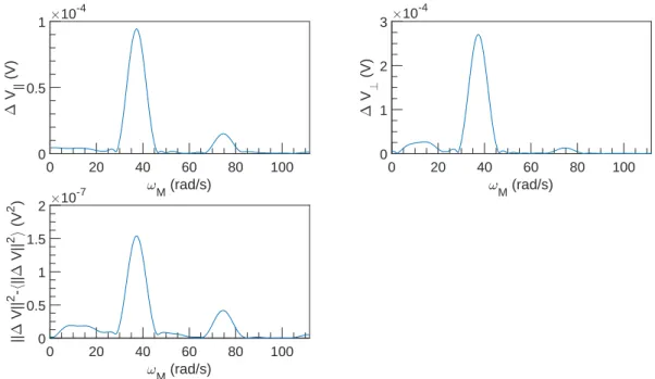
!M (rad/s) 0 20 40 60 80 100 " V || (V) #10-4 0 0.5 1 !M (rad/s) 0 20 40 60 80 100 " V ? (V) #10-4 0 0.5 1 1.5 2 ! M (rad/s) 0 20 40 60 80 100 || " V|| 2 -h || " V|| 2 i (V 2 ) #10 -8 0 2 4 6
Figure 3.20: FFT spectral density of ∆V vs ωM at U = 0.1 m s−1, ω = 3142 rad s−1 and
t (s) 7 8 9 10 11 12 " V || (V) -4 -3 -2 t (s) 7 8 9 10 11 12 " V ? (V) -8 -6 -4 -2 t (s) 7 8 9 10 11 12 || " V|| 2 (V 2 ) #10-7 0 2 4 6 t (s) 7 8 9 10 11 12 I || 0.4201 0.4202 0.4202 0.4203
Figure 3.21: ∆V and I vs t at U = 0.1 m s−1, ω = 4712 rad s−1 and α = 6.9 %.
!M (rad/s) 0 20 40 60 80 100 " V || (V) #10-4 0 0.5 1 !M (rad/s) 0 20 40 60 80 100 " V ? (V) #10-4 0 1 2 3 ! M (rad/s) 0 20 40 60 80 100 || " V|| 2 -h || " V|| 2 i (V 2 ) #10 -7 0 0.5 1 1.5 2
Figure 3.22: FFT spectral density of ∆V vs ωM at U = 0.1 m s−1, ω = 4712 rad s−1 and
t (s) 2 3 4 5 6 7 " V || (V) #10-4 -5 -4 -3 -2 -1 t (s) 2 3 4 5 6 7 " V ? (V) #10-4 -10 -5 0 5 t (s) 2 3 4 5 6 7 || " V|| 2 (V 2 ) #10-6 0 0.5 1 t (s) 2 3 4 5 6 7 I || 0.4044 0.4046 0.4048 0.405
Figure 3.23: ∆V and I vs t at U = 0.1 m s−1, ω = 6283 rad s−1 and α = 6.9 %.
!M (rad/s) 0 20 40 60 80 100 " V || (V) #10-4 0 0.5 1 !M (rad/s) 0 20 40 60 80 100 " V ? (V) #10-4 0 1 2 3 4 ! M (rad/s) 0 20 40 60 80 100 || " V|| 2 -h || " V|| 2 i (V 2 ) #10 -7 0 1 2 3
Figure 3.24: FFT spectral density of ∆V vs ωM at U = 0.1 m s−1, ω = 6283 rad s−1 and
t (s) 2 4 6 8 10 " V || (V) -4 -3 -2 t (s) 2 4 6 8 10 " V ? (V) -15 -10 -5 0 t (s) 2 4 6 8 10 || " V|| 2 (V 2 ) #10-6 0 0.5 1 1.5 t (s) 2 4 6 8 10 I || 0.389 0.3892 0.3894 0.3896 0.3898
Figure 3.25: ∆V and I vs t at U = 0.1 m s−1, ω = 7854 rad s−1 and α = 6.9 %.
!M (rad/s) 0 20 40 60 80 100 " V || (V) #10-5 0 2 4 6 !M (rad/s) 0 20 40 60 80 100 " V ? (V) #10-4 0 2 4 6 ! M (rad/s) 0 20 40 60 80 100 || " V|| 2 -h || " V|| 2 i (V 2 ) #10 -7 0 2 4 6
Figure 3.26: FFT spectral density of ∆V vs ωM at U = 0.1 m s−1, ω = 7854 rad s−1 and
t (s) 5 6 7 8 9 10 " V || (V) #10-4 -4 -3.5 -3 -2.5 -2 t (s) 5 6 7 8 9 10 " V ? (V) #10-4 -15 -10 -5 0 5 t (s) 5 6 7 8 9 10 || " V|| 2 (V 2 ) #10-6 0 0.5 1 1.5 2 t (s) 5 6 7 8 9 10 I || 0.374 0.3745 0.375
Figure 3.27: ∆V and I vs t at U = 0.1 m s−1, ω = 9425 rad s−1 and α = 6.9 %.
!M (rad/s) 0 20 40 60 80 100 " V || (V) #10-5 0 1 2 3 4 !M (rad/s) 0 20 40 60 80 100 " V ? (V) #10-4 0 2 4 6 ! M (rad/s) 0 20 40 60 80 100 || " V|| 2 -h || " V|| 2 i (V 2 ) #10 -7 0 2 4 6
Figure 3.28: FFT spectral density of ∆V vs ωM at U = 0.1 m s−1, ω = 9425 rad s−1 and
t (s) 3 4 5 6 7 8 " V || (V) -4 -3.5 -3 t (s) 3 4 5 6 7 8 " V ? (V) -15 -10 -5 0 t (s) 3 4 5 6 7 8 || " V|| 2 (V 2 ) #10-6 0 0.5 1 1.5 2 t (s) 3 4 5 6 7 8 I || 0.3595 0.36 0.3605 0.361
Figure 3.29: ∆V and I vs t at U = 0.1 m s−1, ω = 10 996 rad s−1 and α = 6.9 %.
!M (rad/s) 0 20 40 60 80 100 " V || (V) #10-5 0 1 2 3 4 !M (rad/s) 0 20 40 60 80 100 " V ? (V) #10-4 0 2 4 6 ! M (rad/s) 0 20 40 60 80 100 || " V|| 2 -h || " V|| 2 i (V 2 ) #10 -7 0 2 4 6 8
Figure 3.30: FFT spectral density of ∆V vs ωM at U = 0.1 m s−1, ω = 10 996 rad s−1
t (s) 3 4 5 6 7 8 " V || (V) #10-4 -4 -3.5 -3 -2.5 t (s) 3 4 5 6 7 8 " V ? (V) #10-4 -15 -10 -5 0 5 t (s) 3 4 5 6 7 8 || " V|| 2 (V 2 ) #10-6 0 1 2 3 t (s) 3 4 5 6 7 8 I || 0.345 0.3455 0.346 0.3465 0.347
Figure 3.31: ∆V and I vs t at U = 0.1 m s−1, ω = 12 566 rad s−1 and α = 6.9 %.
!M (rad/s) 0 20 40 60 80 100 " V || (V) #10-5 0 1 2 3 4 !M (rad/s) 0 20 40 60 80 100 " V ? (V) #10-4 0 2 4 6 8 ! M (rad/s) 0 20 40 60 80 100 || " V|| 2 -h || " V|| 2 i (V 2 ) #10 -6 0 0.5 1
Figure 3.32: FFT spectral density of ∆V vs ωM at U = 0.1 m s−1, ω = 12 566 rad s−1
t (s) 19 20 21 22 23 " V || (V) -2 -1 0 1 t (s) 19 20 21 22 23 " V ? (V) -2 -1 0 1 t (s) 19 20 21 22 23 || " V|| 2 (V 2 ) #10-6 0 1 2 3 4 t (s) 19 20 21 22 23 I || 0.44 0.45 0.46 0.47
Figure 3.33: ∆V and I vs t at U = 1 m s−1, ω = 1571 rad s−1 and α = 6.9 %.
!M (rad/s) 0 200 400 600 800 1000 " V || (V) #10-4 0 0.5 1 !M (rad/s) 0 200 400 600 800 1000 " V ? (V) #10-5 0 2 4 6 ! M (rad/s) 0 200 400 600 800 1000 || " V|| 2 -h || " V|| 2 i (V 2 ) #10 -7 0 0.5 1
Figure 3.34: FFT spectral density of ∆V vs ωM at U = 1 m s−1, ω = 1571 rad s−1 and
t (s) 3 4 5 6 7 " V || (V) #10-4 -10 -5 0 5 t (s) 3 4 5 6 7 " V ? (V) #10-4 -10 -5 0 5 t (s) 3 4 5 6 7 || " V|| 2 (V 2 ) #10-7 0 2 4 6 t (s) 3 4 5 6 7 I || 0.435 0.4355 0.436 0.4365 0.437
Figure 3.35: ∆V and I vs t at U = 1 m s−1, ω = 3142 rad s−1 and α = 6.9 %.
!M (rad/s) 0 200 400 600 800 1000 " V || (V) #10-5 0 2 4 6 8 !M (rad/s) 0 200 400 600 800 1000 " V ? (V) #10-4 0 0.5 1 1.5 ! M (rad/s) 0 200 400 600 800 1000 || " V|| 2 -h || " V|| 2 i (V 2 ) #10 -8 0 2 4 6
Figure 3.36: FFT spectral density of ∆V vs ωM at U = 1 m s−1, ω = 3142 rad s−1 and
t (s) 5 6 7 8 9 " V || (V) -10 -5 0 t (s) 5 6 7 8 9 " V ? (V) -10 -5 0 t (s) 5 6 7 8 9 || " V|| 2 (V 2 ) #10-7 0 2 4 6 8 t (s) 5 6 7 8 9 I || 0.42 0.4202 0.4204 0.4206
Figure 3.37: ∆V and I vs t at U = 1 m s−1, ω = 4712 rad s−1 and α = 6.9 %.
!M (rad/s) 0 200 400 600 800 1000 " V || (V) #10-4 0 0.5 1 !M (rad/s) 0 200 400 600 800 1000 " V ? (V) #10-4 0 1 2 3 ! M (rad/s) 0 200 400 600 800 1000 || " V|| 2 -h || " V|| 2 i (V 2 ) #10 -8 0 2 4 6
Figure 3.38: FFT spectral density of ∆V vs ωM at U = 1 m s−1, ω = 4712 rad s−1 and
t (s) 4 5 6 7 8 " V || (V) #10-4 -6 -4 -2 0 2 t (s) 4 5 6 7 8 " V ? (V) #10-4 -15 -10 -5 0 5 t (s) 4 5 6 7 8 || " V|| 2 (V 2 ) #10-6 0 0.5 1 1.5 t (s) 4 5 6 7 8 I || 0.4044 0.4046 0.4048 0.405
Figure 3.39: ∆V and I vs t at U = 1 m s−1, ω = 6283 rad s−1 and α = 6.9 %.
!M (rad/s) 0 200 400 600 800 1000 " V || (V) #10-5 0 2 4 6 8 !M (rad/s) 0 200 400 600 800 1000 " V ? (V) #10-4 0 1 2 3 4 ! M (rad/s) 0 200 400 600 800 1000 || " V|| 2 -h || " V|| 2 i (V 2 ) #10 -7 0 0.5 1 1.5 2
Figure 3.40: FFT spectral density of ∆V vs ωM at U = 1 m s−1, ω = 6283 rad s−1 and
t (s) 4 5 6 7 8 " V || (V) -6 -4 -2 t (s) 4 5 6 7 8 " V ? (V) -15 -10 -5 0 t (s) 4 5 6 7 8 || " V|| 2 (V 2 ) #10-6 0 0.5 1 1.5 t (s) 4 5 6 7 8 I || 0.3892 0.3894 0.3896 0.3898 0.39
Figure 3.41: ∆V and I vs t at U = 1 m s−1, ω = 7854 rad s−1 and α = 6.9 %.
!M (rad/s) 0 200 400 600 800 1000 " V || (V) #10-5 0 2 4 6 !M (rad/s) 0 200 400 600 800 1000 " V ? (V) #10-4 0 1 2 3 4 ! M (rad/s) 0 200 400 600 800 1000 || " V|| 2 -h || " V|| 2 i (V 2 ) #10 -7 0 1 2 3
Figure 3.42: FFT spectral density of ∆V vs ωM at U = 1 m s−1, ω = 7854 rad s−1 and
t (s) 3 4 5 6 7 " V || (V) #10-4 -6 -4 -2 0 t (s) 3 4 5 6 7 " V ? (V) #10-4 -15 -10 -5 0 5 t (s) 3 4 5 6 7 || " V|| 2 (V 2 ) #10-6 0 0.5 1 1.5 2 t (s) 3 4 5 6 7 I || 0.374 0.3745 0.375 0.3755
Figure 3.43: ∆V and I vs t at U = 1 m s−1, ω = 9425 rad s−1 and α = 6.9 %.
!M (rad/s) 0 200 400 600 800 1000 " V || (V) #10-5 0 1 2 3 4 !M (rad/s) 0 200 400 600 800 1000 " V ? (V) #10-4 0 2 4 6 ! M (rad/s) 0 200 400 600 800 1000 || " V|| 2 -h || " V|| 2 i (V 2 ) #10 -7 0 2 4 6
Figure 3.44: FFT spectral density of ∆V vs ωM at U = 1 m s−1, ω = 9425 rad s−1 and
t (s) 4 5 6 7 " V || (V) -6 -4 -2 t (s) 4 5 6 7 " V ? (V) -15 -10 -5 0 t (s) 4 5 6 7 || " V|| 2 (V 2 ) #10-6 0 1 2 3 t (s) 4 5 6 7 I || 0.3595 0.36 0.3605 0.361
Figure 3.45: ∆V and I vs t at U = 1 m s−1, ω = 10 996 rad s−1 and α = 6.9 %.
!M (rad/s) 0 200 400 600 800 1000 " V || (V) #10-5 0 1 2 3 4 !M (rad/s) 0 200 400 600 800 1000 " V ? (V) #10-4 0 2 4 6 ! M (rad/s) 0 200 400 600 800 1000 || " V|| 2 -h || " V|| 2 i (V 2 ) #10 -7 0 2 4 6
Figure 3.46: FFT spectral density of ∆V vs ωM at U = 1 m s−1, ω = 10 996 rad s−1 and
t (s) 6 7 8 9 " V || (V) #10-4 -6 -4 -2 0 t (s) 6 7 8 9 " V ? (V) #10-3 -2 -1 0 1 t (s) 6 7 8 9 || " V|| 2 (V 2 ) #10-6 0 1 2 3 t (s) 6 7 8 9 I || 0.345 0.3455 0.346 0.3465 0.347
Figure 3.47: ∆V and I vs t at U = 1 m s−1, ω = 12 566 rad s−1 and α = 6.9 %.
!M (rad/s) 0 200 400 600 800 1000 " V || (V) #10-5 0 1 2 3 !M (rad/s) 0 200 400 600 800 1000 " V ? (V) #10-4 0 2 4 6 ! M (rad/s) 0 200 400 600 800 1000 || " V|| 2 -h || " V|| 2 i (V 2 ) #10 -7 0 2 4 6 8
Figure 3.48: FFT spectral density of ∆V vs ωM at U = 1 m s−1, ω = 12 566 rad s−1 and
t (s) 0 50 100 150 200 " V || (V) -6 -4 -2 0 t (s) 0 50 100 150 200 " V ? (V) -10 -5 0 t (s) 0 50 100 150 200 || " V|| 2 (V 2 ) #10-7 0 2 4 6 t (s) 0 50 100 150 200 I || 0.434 0.435 0.436 0.437
Figure 3.49: ∆V and I vs t at U = 10−3m s−1, ω = 3142 rad s−1 and α = 6.9 %.
!M (rad/s) 0 0.2 0.4 0.6 0.8 1 " V || (V) #10-4 0 0.5 1 !M (rad/s) 0 0.2 0.4 0.6 0.8 1 " V ? (V) #10-4 0 0.5 1 1.5 2 ! M (rad/s) 0 0.2 0.4 0.6 0.8 1 || " V|| 2 -h || " V|| 2 i (V 2 ) #10 -8 0 2 4 6
Figure 3.50: FFT spectral density of ∆V vs ωM at U = 10−3m s−1, ω = 3142 rad s−1
t (s) 0 50 100 150 200 " V || (V) #10-4 -4 -3 -2 -1 t (s) 0 50 100 150 200 " V ? (V) #10-4 -10 -5 0 5 t (s) 0 50 100 150 200 || " V|| 2 (V 2 ) #10-6 0 0.5 1 t (s) 0 50 100 150 200 I || 0.4044 0.4045 0.4046 0.4047 0.4048
Figure 3.51: ∆V and I vs t at U = 10−3m s−1, ω = 6283 rad s−1 and α = 6.9 %.
!M (rad/s) 0 0.2 0.4 0.6 0.8 1 " V || (V) #10-4 0 0.5 1 !M (rad/s) 0 0.2 0.4 0.6 0.8 1 " V ? (V) #10-4 0 1 2 3 4 ! M (rad/s) 0 0.2 0.4 0.6 0.8 1 || " V|| 2 -h || " V|| 2 i (V 2 ) #10 -7 0 1 2 3 4
Figure 3.52: FFT spectral density of ∆V vs ωM at U = 10−3m s−1, ω = 6283 rad s−1
t (s) 0 50 100 150 " V || (V) -6 -4 -2 0 t (s) 0 50 100 150 " V ? (V) -10 -5 0 t (s) 0 50 100 150 || " V|| 2 (V 2 ) #10-7 0 2 4 6 t (s) 0 50 100 150 I || 0.434 0.435 0.436 0.437
Figure 3.53: ∆V and I vs t at U = 3 × 10⁻³m s−1, ω = 3142 rad s−1 and α = 6.9 %.
!M (rad/s) 0 1 2 3 " V || (V) #10-4 0 0.5 1 !M (rad/s) 0 1 2 3 " V ? (V) #10-4 0 0.5 1 1.5 2 ! M (rad/s) 0 1 2 3 || " V|| 2 -h || " V|| 2 i (V 2 ) #10 -8 0 2 4 6
Figure 3.54: FFT spectral density of ∆V vs ωM at U = 3 × 10⁻³m s−1, ω = 3142 rad s−1
t (s) 0 50 100 150 " V || (V) #10-4 -4 -3 -2 -1 t (s) 0 50 100 150 " V ? (V) #10-4 -10 -5 0 5 t (s) 0 50 100 150 || " V|| 2 (V 2 ) #10-6 0 0.5 1 t (s) 0 50 100 150 I || 0.4044 0.4046 0.4048 0.405
Figure 3.55: ∆V and I vs t at U = 3 × 10⁻³m s−1, ω = 6283 rad s−1 and α = 6.9 %.
!M (rad/s) 0 1 2 3 " V || (V) #10-4 0 0.5 1 !M (rad/s) 0 1 2 3 " V ? (V) #10-4 0 1 2 3 4 ! M (rad/s) 0 1 2 3 || " V|| 2 -h || " V|| 2 i (V 2 ) #10 -7 0 1 2 3 4
Figure 3.56: FFT spectral density of ∆V vs ωM at U = 3 × 10⁻³m s−1, ω = 6283 rad s−1
t (s) 0 10 20 30 40 " V || (V) -6 -4 -2 0 t (s) 0 10 20 30 40 " V ? (V) -10 -5 0 t (s) 0 10 20 30 40 || " V|| 2 (V 2 ) #10-7 0 2 4 6 t (s) 0 10 20 30 40 I || 0.434 0.435 0.436 0.437
Figure 3.57: ∆V and I vs t at U = 10−2m s−1, ω = 3142 rad s−1 and α = 6.9 %.
!M (rad/s) 0 2 4 6 8 10 " V || (V) #10-4 0 0.5 1 !M (rad/s) 0 2 4 6 8 10 " V ? (V) #10-4 0 0.5 1 1.5 2 ! M (rad/s) 0 2 4 6 8 10 || " V|| 2 -h || " V|| 2 i (V 2 ) #10 -8 0 2 4 6
Figure 3.58: FFT spectral density of ∆V vs ωM at U = 10−2m s−1, ω = 3142 rad s−1
t (s) 10 20 30 40 50 " V || (V) #10-4 -5 -4 -3 -2 -1 t (s) 10 20 30 40 50 " V ? (V) #10-4 -10 -5 0 5 t (s) 10 20 30 40 50 || " V|| 2 (V 2 ) #10-6 0 0.5 1 t (s) 10 20 30 40 50 I || 0.4045 0.4046 0.4047 0.4048 0.4049
Figure 3.59: ∆V and I vs t at U = 10−2m s−1, ω = 6283 rad s−1 and α = 6.9 %.
!M (rad/s) 0 2 4 6 8 10 " V || (V) #10-4 0 0.5 1 !M (rad/s) 0 2 4 6 8 10 " V ? (V) #10-4 0 1 2 3 4 ! M (rad/s) 0 2 4 6 8 10 || " V|| 2 -h || " V|| 2 i (V 2 ) #10 -7 0 1 2 3 4
Figure 3.60: FFT spectral density of ∆V vs ωM at U = 10−2m s−1, ω = 6283 rad s−1
t (s) 0 5 10 15 " V || (V) -6 -4 -2 0 t (s) 0 5 10 15 " V ? (V) -10 -5 0 t (s) 0 5 10 15 || " V|| 2 (V 2 ) #10-7 0 2 4 6 t (s) 0 5 10 15 I || 0.434 0.435 0.436 0.437
Figure 3.61: ∆V and I vs t at U = 3 × 10⁻²m s−1, ω = 3142 rad s−1 and α = 6.9 %.
!M (rad/s) 0 10 20 30 " V || (V) #10-4 0 0.5 1 !M (rad/s) 0 10 20 30 " V ? (V) #10-4 0 0.5 1 1.5 2 ! M (rad/s) 0 10 20 30 || " V|| 2 -h || " V|| 2 i (V 2 ) #10 -8 0 2 4 6
Figure 3.62: FFT spectral density of ∆V vs ωM at U = 3 × 10⁻²m s−1, ω = 3142 rad s−1
t (s) 0 5 10 15 20 " V || (V) #10-4 -5 -4 -3 -2 -1 t (s) 0 5 10 15 20 " V ? (V) #10-4 -10 -5 0 5 t (s) 0 5 10 15 20 || " V|| 2 (V 2 ) #10-6 0 0.5 1 t (s) 0 5 10 15 20 I || 0.4044 0.4046 0.4048 0.405
Figure 3.63: ∆V and I vs t at U = 3 × 10⁻²m s−1, ω = 6283 rad s−1 and α = 6.9 %.
!M (rad/s) 0 10 20 30 " V || (V) #10-4 0 0.5 1 !M (rad/s) 0 10 20 30 " V ? (V) #10-4 0 1 2 3 4 ! M (rad/s) 0 10 20 30 || " V|| 2 -h || " V|| 2 i (V 2 ) #10 -7 0 1 2 3 4
Figure 3.64: FFT spectral density of ∆V vs ωM at U = 3 × 10⁻²m s−1, ω = 6283 rad s−1
t (s) 4 6 8 10 " V || (V) -6 -4 -2 0 t (s) 4 6 8 10 " V ? (V) -10 -5 0 t (s) 4 6 8 10 || " V|| 2 (V 2 ) #10-7 0 2 4 6 t (s) 4 6 8 10 I || 0.434 0.435 0.436 0.437
Figure 3.65: ∆V and I vs t at U = 0.1 m s−1, ω = 3142 rad s−1 and α = 6.9 %.
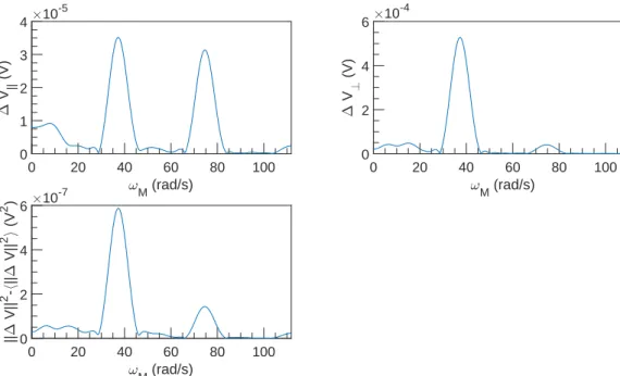
!M (rad/s) 0 20 40 60 80 100 " V || (V) #10-4 0 0.5 1 !M (rad/s) 0 20 40 60 80 100 " V ? (V) #10-4 0 0.5 1 1.5 2 ! M (rad/s) 0 20 40 60 80 100 || " V|| 2 -h || " V|| 2 i (V 2 ) #10 -8 0 2 4 6
Figure 3.66: FFT spectral density of ∆V vs ωM at U = 0.1 m s−1, ω = 3142 rad s−1 and
t (s) 2 3 4 5 6 7 " V || (V) #10-4 -5 -4 -3 -2 -1 t (s) 2 3 4 5 6 7 " V ? (V) #10-4 -10 -5 0 5 t (s) 2 3 4 5 6 7 || " V|| 2 (V 2 ) #10-6 0 0.5 1 t (s) 2 3 4 5 6 7 I || 0.4044 0.4046 0.4048 0.405
Figure 3.67: ∆V and I vs t at U = 0.1 m s−1, ω = 6283 rad s−1 and α = 6.9 %.
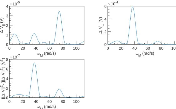
!M (rad/s) 0 20 40 60 80 100 " V || (V) #10-4 0 0.5 1 !M (rad/s) 0 20 40 60 80 100 " V ? (V) #10-4 0 1 2 3 4 ! M (rad/s) 0 20 40 60 80 100 || " V|| 2 -h || " V|| 2 i (V 2 ) #10 -7 0 1 2 3
Figure 3.68: FFT spectral density of ∆V vs ωM at U = 0.1 m s−1, ω = 6283 rad s−1 and
t (s) 2 3 4 5 6 " V || (V) -6 -4 -2 0 t (s) 2 3 4 5 6 " V ? (V) -10 -5 0 t (s) 2 3 4 5 6 || " V|| 2 (V 2 ) #10-7 0 2 4 6 t (s) 2 3 4 5 6 I || 0.435 0.4355 0.436 0.4365 0.437
Figure 3.69: ∆V and I vs t at U = 0.25 m s−1, ω = 3142 rad s−1 and α = 6.9 %.
!M (rad/s) 0 50 100 150 200 250 " V || (V) #10-4 0 0.5 1 !M (rad/s) 0 50 100 150 200 250 " V ? (V) #10-4 0 0.5 1 1.5 2 ! M (rad/s) 0 50 100 150 200 250 || " V|| 2 -h || " V|| 2 i (V 2 ) #10 -8 0 1 2 3 4
Figure 3.70: FFT spectral density of ∆V vs ωM at U = 0.25 m s−1, ω = 3142 rad s−1
t (s) 3 4 5 6 7 8 " V || (V) #10-4 -5 -4 -3 -2 -1 t (s) 3 4 5 6 7 8 " V ? (V) #10-4 -10 -5 0 5 t (s) 3 4 5 6 7 8 || " V|| 2 (V 2 ) #10-6 0 0.5 1 t (s) 3 4 5 6 7 8 I || 0.4046 0.4047 0.4048 0.4049 0.405
Figure 3.71: ∆V and I vs t at U = 0.25 m s−1, ω = 6283 rad s−1 and α = 6.9 %.
!M (rad/s) 0 50 100 150 200 250 " V || (V) #10-4 0 0.5 1 !M (rad/s) 0 50 100 150 200 250 " V ? (V) #10-4 0 1 2 3 4 ! M (rad/s) 0 50 100 150 200 250 || " V|| 2 -h || " V|| 2 i (V 2 ) #10 -7 0 1 2 3
Figure 3.72: FFT spectral density of ∆V vs ωM at U = 0.25 m s−1, ω = 6283 rad s−1
t (s) 8 9 10 11 " V || (V) -10 -5 0 t (s) 8 9 10 11 " V ? (V) -10 -5 0 t (s) 8 9 10 11 || " V|| 2 (V 2 ) #10-7 0 2 4 6 t (s) 8 9 10 11 I || 0.435 0.4355 0.436 0.4365 0.437
Figure 3.73: ∆V and I vs t at U = 0.5 m s−1, ω = 3142 rad s−1 and α = 6.9 %.
!M (rad/s) 0 100 200 300 400 500 " V || (V) #10-4 0 0.5 1 !M (rad/s) 0 100 200 300 400 500 " V ? (V) #10-4 0 0.5 1 1.5 2 ! M (rad/s) 0 100 200 300 400 500 || " V|| 2 -h || " V|| 2 i (V 2 ) #10 -8 0 0.5 1 1.5 2
Figure 3.74: FFT spectral density of ∆V vs ωM at U = 0.5 m s−1, ω = 3142 rad s−1 and
t (s) 5 6 7 8 9 " V || (V) #10-4 -6 -4 -2 0 t (s) 5 6 7 8 9 " V ? (V) #10-4 -10 -5 0 5 t (s) 5 6 7 8 9 || " V|| 2 (V 2 ) #10-6 0 0.5 1 1.5 t (s) 5 6 7 8 9 I || 0.4046 0.4047 0.4048 0.4049 0.405
Figure 3.75: ∆V and I vs t at U = 0.5 m s−1, ω = 6283 rad s−1 and α = 6.9 %.
!M (rad/s) 0 100 200 300 400 500 " V || (V) #10-4 0 0.5 1 !M (rad/s) 0 100 200 300 400 500 " V ? (V) #10-4 0 1 2 3 4 ! M (rad/s) 0 100 200 300 400 500 || " V|| 2 -h || " V|| 2 i (V 2 ) #10 -7 0 1 2 3
Figure 3.76: FFT spectral density of ∆V vs ωM at U = 0.5 m s−1, ω = 6283 rad s−1 and
t (s) 2 3 4 5 " V || (V) -10 -5 0 t (s) 2 3 4 5 " V ? (V) -10 -5 0 t (s) 2 3 4 5 || " V|| 2 (V 2 ) #10-7 0 2 4 6 t (s) 2 3 4 5 I || 0.435 0.4355 0.436 0.4365 0.437
Figure 3.77: ∆V and I vs t at U = 0.75 m s−1, ω = 3142 rad s−1 and α = 6.9 %.
!M (rad/s) 0 200 400 600 800 " V || (V) #10-4 0 0.5 1 !M (rad/s) 0 200 400 600 800 " V ? (V) #10-4 0 0.5 1 1.5 ! M (rad/s) 0 200 400 600 800 || " V|| 2 -h || " V|| 2 i (V 2 ) #10 -8 0 1 2 3
Figure 3.78: FFT spectral density of ∆V vs ωM at U = 0.75 m s−1, ω = 3142 rad s−1
t (s) 5 6 7 8 " V || (V) #10-4 -6 -4 -2 0 t (s) 5 6 7 8 " V ? (V) #10-4 -15 -10 -5 0 5 t (s) 5 6 7 8 || " V|| 2 (V 2 ) #10-6 0 0.5 1 1.5 t (s) 5 6 7 8 I || 0.4046 0.4048 0.405 0.4052
Figure 3.79: ∆V and I vs t at U = 0.75 m s−1, ω = 6283 rad s−1 and α = 6.9 %.
!M (rad/s) 0 200 400 600 800 " V || (V) #10-5 0 2 4 6 8 !M (rad/s) 0 200 400 600 800 " V ? (V) #10-4 0 1 2 3 4 ! M (rad/s) 0 200 400 600 800 || " V|| 2 -h || " V|| 2 i (V 2 ) #10 -7 0 0.5 1 1.5 2
Figure 3.80: FFT spectral density of ∆V vs ωM at U = 0.75 m s−1, ω = 6283 rad s−1
t (s) 4 5 6 7 " V || (V) -10 -5 0 t (s) 4 5 6 7 " V ? (V) -10 -5 0 t (s) 4 5 6 7 || " V|| 2 (V 2 ) #10-7 0 2 4 6 t (s) 4 5 6 7 I || 0.435 0.4355 0.436 0.4365 0.437
Figure 3.81: ∆V and I vs t at U = 1 m s−1, ω = 3142 rad s−1 and α = 6.9 %.
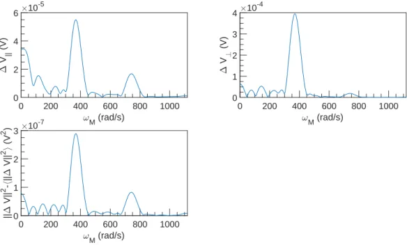
!M (rad/s) 0 200 400 600 800 1000 " V || (V) #10-4 0 0.5 1 !M (rad/s) 0 200 400 600 800 1000 " V ? (V) #10-4 0 0.5 1 1.5 ! M (rad/s) 0 200 400 600 800 1000 || " V|| 2 -h || " V|| 2 i (V 2 ) #10 -8 0 2 4 6
Figure 3.82: FFT spectral density of ∆V vs ωM at U = 1 m s−1, ω = 3142 rad s−1 and
t (s) 4 5 6 7 8 " V || (V) #10-4 -6 -4 -2 0 2 t (s) 4 5 6 7 8 " V ? (V) #10-4 -15 -10 -5 0 5 t (s) 4 5 6 7 8 || " V|| 2 (V 2 ) #10-6 0 0.5 1 1.5 t (s) 4 5 6 7 8 I || 0.4046 0.4047 0.4048 0.4049 0.405
Figure 3.83: ∆V and I vs t at U = 1 m s−1, ω = 6283 rad s−1 and α = 6.9 %.
!M (rad/s) 0 200 400 600 800 1000 " V || (V) #10-5 0 2 4 6 8 !M (rad/s) 0 200 400 600 800 1000 " V ? (V) #10-4 0 1 2 3 4 ! M (rad/s) 0 200 400 600 800 1000 || " V|| 2 -h || " V|| 2 i (V 2 ) #10 -7 0 0.5 1 1.5 2
Figure 3.84: FFT spectral density of ∆V vs ωM at U = 1 m s−1, ω = 6283 rad s−1 and