HAL Id: tel-03147834
https://hal.archives-ouvertes.fr/tel-03147834
Submitted on 21 Feb 2021
HAL is a multi-disciplinary open access
archive for the deposit and dissemination of
sci-entific research documents, whether they are
pub-lished or not. The documents may come from
teaching and research institutions in France or
abroad, or from public or private research centers.
L’archive ouverte pluridisciplinaire HAL, est
destinée au dépôt et à la diffusion de documents
scientifiques de niveau recherche, publiés ou non,
émanant des établissements d’enseignement et de
recherche français ou étrangers, des laboratoires
publics ou privés.
in vascular surgery
Hugo Gangloff
To cite this version:
Hugo Gangloff. Probabilistic models for image processing: applications in vascular surgery. Medical
Imaging. Université de Strasbourg, 2020. English. �tel-03147834�
Université de Strasbourg
École doctorale MSII
Laboratoire ICube - UMR 7357
THÈSE
présentée par :
Hugo GANGLOFF
soutenue le :
15 décembre 2020
pour l’obtention du grade de : docteur de l’Université de Strasbourg
Discipline / Spécialité : signal, image, automatique, robotique
Probabilistic models for image processing:
applications in vascular surgery
THÈSE dirigée par :
Christophe Collet
Professeur, Université de Strasbourg
Directeur de thèse
Nabil Chakfé
Professeur, Université de Strasbourg
Co-directeur de thèse
RAPPORTEURS :
Isabelle Bloch
Professeur, Télécom Paris
Cédric Richard
Professeur, Université Nice Sophia Antipolis
AUTRES MEMBRES DU JURY :
In the morning all the birds are chirping and everything is going on. I grab a coffee and get to work. Then when I get tired, I take off. If I run out of ideas, I go for a run, and things fall into place.
Acknowledgements
Je te tiens tout d’abord à remercier Isabelle Bloch et Cédric Richard d’avoir accepté d’être les rapporteurs de mon travail. Je remercie également Wojciech Pieczynski d’avoir présidé mon jury de thèse.
Merci à Mauro Gargiulo (Professeur à l’Université de Bologne) d’avoir honoré le jury de sa présence, en qualité de membre invité.
Un grand merci à mes directeurs de thèse, Christophe Collet et Nabil Chakfé, et à mon encadrant de thèse, Emmanuel Monfrini. Depuis le début, ils m’ont fait confiance, m’ont encouragé et soutenu. Merci de m’avoir ouvert les portes des laboratoires ICube et Geprovas pour ces trois intenses années de thèse qui viennent de s’écouler...
Merci à Jean-Baptiste Courbot, qui m’a transmis une partie de ses connais-sances et de son expérience d’enseignant-chercheur, en donnant beaucoup de son temps et de son énergie.
Merci à ma famille. En particulier, la présence sans faille de mes deux mamies et de mes parents, depuis le tout début, a été essentielle à la réussite de cette thèse. Merci à ma sœur, qui démontre que le succès peut prendre une infinité de formes.
Finalement, je veux dire merci à toutes les personnes que j’ai croisées pendant ces dernières années, je suis certain d’avoir appris quelque chose de chacune de nos rencontres. C’était un plaisir de passer du temps à vos côtés et d’avancer, dans la thèse ou dans toutes les autres aventures qu’offre la vie. Donner une liste de noms me semble risqué et grandement insatisfaisant ; j’ai confiance dans le fait que vous vous reconnaîtrez...
Contents
Acknowledgements v
Contents vii
List of Acronyms xi
List of Notations xiii
Résumé étendu 1
Introduction 9
Chapter 1. Main concepts in probabilistic modeling 23
1.1. Introduction . . . 24
1.2. Graphical modeling . . . 24
1.2.1. Main definitions . . . 24
1.2.2. Directed Graphical Models . . . 25
1.2.3. Undirected Graphical Models . . . 27
1.3. Inference in probabilistic models . . . 28
1.3.1. Exact inference . . . 29
1.3.2. Approximate inference . . . 30
1.4. Parameter estimation . . . 30
1.4.1. Maximum Likelihood estimation . . . 31
1.4.2. Estimation for DGMs . . . 31
1.4.3. Parameter estimation for UGMs . . . 32
1.5. Probabilistic models for image segmentation . . . 33
1.5.1. Definitions and context . . . 33
1.5.2. Bayesian image segmentation . . . 34
1.5.3. Discriminative and generative models . . . 35
1.6. Hidden Markov Models . . . 35
1.6.1. Main families of HMMs . . . 36
1.6.2. Pairwise and Triplet extensions . . . 39
1.7. Conclusion . . . 39
Chapter 2. Gaussian Pairwise Markov Fields 41 2.1. Introduction . . . 42
2.2. Gaussian Pairwise Markov Fields . . . 44
2.2.1. Model definition . . . 44
2.2.2. Description of the GPMF distribution . . . 45
2.2.4. The model parameters . . . 47
2.3. Related models: the PMF model family . . . 48
2.4. Parameter estimation . . . 50
2.4.1. Stochastic Parameter Estimation . . . 50
2.5. Experiments and Results . . . 53
2.5.1. Improved sampling with Tempered-Gibbs sampler . . . 54
2.5.2. Supervised segmentation of semi-real images with the PMF models . . . 57
2.5.3. Unsupervised segmentation on semi-real images . . . 57
2.5.4. On real world images . . . 60
2.6. Conclusion . . . 63
Chapter 3. Spatial Triplet Markov Trees 67 3.1. Introduction . . . 68
3.2. Markov Tree models . . . 68
3.2.1. Hidden Markov Trees . . . 68
3.2.2. Spatial Triplet Markov Trees . . . 69
3.3. Image segmentation . . . 75
3.3.1. The Potts-like transition distributions . . . 75
3.3.2. Iterative Parameter Estimation for Trees . . . 77
3.3.3. Experiments and Results . . . 78
3.4. STMTs for Auxiliary Variational Inference in SBNs . . . 81
3.4.1. Spatial Bayes Networks . . . 83
3.4.2. Variational inference . . . 86
3.4.3. Mean Field Variational Inference in SBNs . . . 87
3.4.4. Markov Tree Variational Inference in SBNs . . . 88
3.4.5. Auxiliary variable Variational Inference . . . 88
3.4.6. STMT auxiliary variable Variational Inference in SBNs 90 3.4.7. Experiments & Results . . . 91
3.5. Conclusion . . . 93
Chapter 4. Image segmentation with Deep Learning and Conditional Random Fields 97 4.1. Introduction . . . 98
4.2. Convolutional Neural Networks . . . 101
4.2.1. The Deep-Learning approach . . . 101
4.2.2. Network definition . . . 101
4.3. Fully-connected Conditional Random Fields . . . 104
4.3.1. Model definition . . . 104
4.3.2. Optimized Mean Field Variational Inference for fcCRFs 105 4.4. Markov Chain Variational Inference for fcCRFs . . . 107
4.4.1. Markov Chains for image processing . . . 108
4.4.2. Scanning the data with Markov Chains . . . 108
4.5. Experiments and Results . . . 111
Contents 4.5.2. Experimental comparisons of MF VI and MC VI on
semi-real images . . . 112
4.5.3. Post-processing with fcCRFs . . . 115
4.6. Conclusion . . . 120
Chapter 5. Applications to vascular surgery 123 5.1. Introduction . . . 124
5.2. Unsupervised segmentation of stents corrupted by artifacts . . 124
5.2.1. Context and motivation . . . 124
5.2.2. A HMC dedicated to handling strong artifacts . . . 126
5.2.3. Results . . . 129
5.3. Unsupervised segmentation of the organic material and calcifi-cations . . . 133
5.3.1. Organic material segmentation with GPMFs . . . 133
5.3.2. Unsupervised calcification segmentation with STMTs . . 137
5.4. Histological segmentation of microCT with Deep Learning . . . 141
5.4.1. Motivation . . . 141
5.4.2. Protocol and database construction . . . 141
5.4.3. Results . . . 143
5.5. Conclusion . . . 148
Conclusions and Perspectives 149 Appendix A. Main algorithms in probabilistic modeling 153 Appendix B. Complements on GMRFs 157 B.1. Stationary GRFs and GMRFs . . . 157
B.2. Spectral methods for GMRFs . . . 158
B.2.1. Circulant matrices . . . 158
B.2.2. Spectral properties . . . 159
B.2.3. Torus assumption for GRFs and GMRFs . . . 159
B.2.4. Indices ordering . . . 160
B.3. Application to GMRF simulation . . . 161
Appendix C. Complements on GPMF 163 C.1. Derivation of the single site equations . . . 163
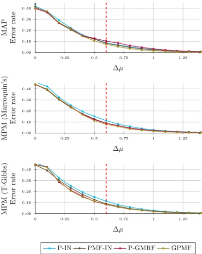
C.2. T-Gibbs sampler complementary experiment . . . 165
Appendix D. Complements on Variational Inference 169 D.1. Mean Field Variational Inference in SBNs . . . 169
D.2. Markov Tree Variational Inference in SBNs . . . 172
D.3. STMT auxiliary variable Variational Inference in SBNs . . . 175
Appendix E. Complements on fcCRFs 179 E.1. Augmented space for the bilateral kernel computations . . . 179
Appendix F. Complements on the applications to vascular surgery 185
F.1. Fine stent segmentation: exponential mixture models . . . 185
Bibliography 189
List of Figures 209
List of Tables 211
List of Acronyms
Probabilistic Graphical Models
CN Correlated Noise.
CRF Conditional Random Field. DAG Directed Acyclic Graph. DGM Directed Graphical Model.
fcCRF fully-connected Conditional Random Field. GMM Gaussian Mixture Model.
GMRF Gaussian Markov Random Field. GMRF Gaussian Random Field.
GPMF Gaussian Pairwise Markov Field. HMC Hidden Markov Chain.
HMF Hidden Markov Field. HMM Hidden Markov Model. HMT Hidden Markov Tree. IN Independent Noise. MC Markov Chain.
MoE Mixture of exponentials. MoG Mixture of Gaussians. MRF Markov Random Field. MT Markov Tree.
P-IN Potts-Independent Noise. PMF Pairwise Markov Field. SBN Spatial Bayes Network. STMT Spatial Triplet Markov Tree. UGM Undirected Graphical Model. UN Uncorrelated Noise.
Others
AUC Area Under Curve.
Ba Background.
BHC Beam Hardening Correction. BIC Bayesian Information Criterion. BM3D Block-Matching 3D.
CNN Convolutional Neural Network. CT Computed Tomography. CVD Cardiovascular Disease. DL Deep Learning. EM Expectation Maximization. FB Forward Backward. FN False Negative. FP False Positive. FT Fatty Tissue. GC Graph-Cut.
IPET Iterative Parameter Estimation for Trees. KL Kullback Leibler.
LLS Linear Least Square. MAP Maximum A Posteriori. MAR Metal Artifact Reduction. MCMC Markov Chain Monte Carlo.
mCT micro-Computed Tomography (also microCT). MF Mean Field.
ML Maximum Likelihood. MPM Maximum Posterior Mode. MRI Magnetic Resonance Imaging. NC Nodular Calcification.
PET Positron Emission Tomography. PR Precision Recall.
pyIS pyImSegm.
RNN Recurrent Neural Network. ROC Receiver Operating Characteristic.
RORPO Ranking the Orientation Responses of Path Opera-tor.
SA Simulated Annealing. SC Sheet Calcification.
SEM Stochastic Expectation Maximization. SH Specimen Holder.
SPD Symmetric Positive Definite. SPE Stochastic Parameter Estimation. ST Soft Tissue.
T-Gibbs Tempered-Gibbs. UD Upward Downward. VI Variational Inference.
List of Notations
General
a Light lower case letters represent scalars or func-tions.
a a a a
aaa Bold lower case letters represent vectors. A Capital letters represent matrices. ∝ Equality up to a constant factor. δ Kronecker function.
1 Indicator function.
| · | Cardinal of a set or absolute value of scalar. k.k A distance function (Euclidean, `1, ...). det(·) Determinant of a matrix.
·T Transpose operator on vectors or matrices.
× Product (explicit notation) or Cartesian product. • Element-wise power.
Element-wise multiplication.
DFT2(·) Bidimensional Discrete Fourier Transform. IDFT2(·) Bidimensional Inverse Fourier Transform. <(·) Real part of complex number.
=(·) Imaginary part of complex number. ∪ Set union operator.
∩ Set intersection operator. ∧ Logical and operator. ∨ Logical or operator.
Graph Theory
G A graph.
E Set of edges of a graph. S Set of vertices of a graph. Ns Neighborhood of site s.
P(s) Set of parents of s. s− A parent vertice of s.
¯
S Set of vertices with at least a parent vertice. s
s s
ssss++ The set of all descendants of s.
s s s
Probability Theory
X Capital letters represent random variables. x The realization of the random variable X. X X X X X X
X Bold capital letters represent random vectors. E[X] Expectation of random variable X.
KL(q||p) Kullback Leibler divergence between distributions q and p.
PX The law of random variable X.
p(x) -Discrete case: the probability p({X = x}).
-Continuous case: the probability density of random variable X.
N (·, ·) Normal (Gaussian) density function.
(first argument is the mean and second the vari-ance).
Résumé étendu
Introduction
Les maladies cardiovasculaires sont la première cause de mortalité dans le monde. Les coûts de ces maladies pour les sociétés sont humain et économique, ils sont déjà importants (chiffrés en plusieurs centaines de milliards de dollars) et ne cessent de croître1 2. Le vieillissement et l’augmentation de la population
mondiale sont des facteurs contribuant à l’augmentation de ces pathologies. Pour y faire face, la recherche est poussée à mieux connaître ces maladies et développer de nouveaux traitements plus efficaces.
Dans ce contexte, les approches modernes en chirurgie vasculaires sont basées sur des opérations mini-invasives guidées par l’image et sur l’implantation de biomatériaux (dont l’élément le plus connu est le stent). On parle de chirurgie endovasculaire. Ces nouveaux types d’intervention offrent une alternative à la chirurgie ouverte classique. Cependant, la chirurgie endovasculaire, déjà largement pratiquée, soulève des questions auxquelles la recherche n’a actuelle-ment que des réponses trop partielles. Ces questions concernent aussi bien le comportement mécanique des biomatériaux dans le corps du patient et leur implantation par le chirurgien, que la correction d’images scanner illisibles et l’utilisation per-opératoire de ces images.
Les problématiques présentées ci-dessus relèvent d’une recherche fortement pluri-disciplinaire. Dans cette thèse, nous présentons des contributions aux traitement des images médicales. Ces contributions ont pour but de perme-ttre la création de nouveaux outils qui doivent servir à d’autres chercheurs (biomécaniciens, chirurgiens, spécialistes du textile, radiologues, histopatholo-gistes, ...) pour, in fine, mieux connaître les maladies cardiovasculaires, leur traitement et leur prévention. Nos contributions sont liées à une principale application : celle de la segmentation des images médicales.
Les images que nous traitons dans la thèse sont de type Computed Tomogra-phy(CT) ou micro-Computed Tomography (mCT). Les principaux défis dans la segmentation des images médicales en chirurgie vasculaire concernent la com-plexité et les dégradations subies par images à rayons-X lorsque celles-ci con-tiennent un biomatériau métallique, la disponibilité limitée des données et la taille des données à traiter. Dans la section suivante, nous décrivons plus en dé-tails ces problèmes, en mettant en avant les méthodes graphiques probabilistes utilisées pendant la thèse pour les traiter. La Figure0.2illustre un cas typique
1https://healthmetrics.heart.org/wp-content/uploads/2017/10/
Cardiovascular-Disease-A-Costly-Burden.pdf
2https://www.bhf.org.uk/what-we-do/our-research/heart-statistics/
Calcifications Stent Artifacts
Figure 0.2.: Coupe de CT scan typique des données à traiter. Le stent se trouve dans un environnement complexe, entouré de calcifications et d’artéfacts. Notons qu’un bruit corrélé est une modélisation per-tinente de ce phénomène.
des données de chirurgie vasculaire que nous souhaitons pouvoir segmenter.
Méthodes
Dans les modèles graphiques probabilites appliqués à la segmentation des im-ages, des sommets du graphe sont associés à des variables aléatoires qui représen-tent l’image observée, et d’autres sommets sont associés à des variables aléa-toires qui correspondent aux classes dans l’image segmentée. Les arêtes du graphe représentent une relation de dépendance entre les deux variables reliées. Les arêtes peuvent être orientées ou non-orientées ce qui modifie la formulation probabiliste du modèle (Murphy, 2012).
Les modèles graphiques probabilistes les plus connus pour la segmentation sont ceux de la famille des modèles de Markov cachés (Baum and Petrie, 1966). Parmi les modèles de Markov cachés les plus populaires, nous notons les chaînes et arbres de Markov (Baum and Petrie, 1966) (Laferté et al., 2000) (modèles graphiques orientés) et les champs de Markov (Kato and Zerubia, 2012) (modèle graphique non-orienté). Nous étudions largement ces modèles et leurs extensions : les modèles de Markov cachés couples et triplets ( Pieczyn-ski and Tebbache, 2000) (Lanchantin et al., 2011) (Gorynin, Gangloff, et al., 2018). Les modèles probabilistes markoviens offrent un moyen simple et intuitif d’introduire de la dépendance entre les pixels de l’image, ils sont une réponse pertinente aux problématiques posées par les images étudiées pendant la thèse. Nous passons maintenant en revue les principales notions théoriques sur les modèles probabilistes graphiques, à la lumière des problématiques propres à notre application.
Modèles probabilistes et segmentation d’images bruitées
Une problématique particulière à laquelle nous devons faire face est celle des artéfacts. Lors de l’acquisition des images à rayons-X, les biomatériauxmé-talliques présents dans le corps du patient vont intéragir avec les rayons-X ce qui va créer, à la sortie de l’algorithme de reconstruction CT, de forts arté-facts. Ces derniers empêchent de discerner facilement l’anatomie environnante. D’un point du vue du traitement du signal les artéfacts peuvent être modélisés comme du bruit spatialement corrélé. Ce type bruit peut être naturellement modélisé dans certains modèles graphiques probabilistes comme les nouveaux modèles de Markov couples et triplets (Gorynin, Gangloff, et al., 2018) qui sont présentés dans la thèse. En parallèle, les corrélations spatiales sont classique-ment étudiées dans les modèles de type Gaussian Markov Random Fields (Rue and Held, 2005) (GMRF) qui sont également étudiés dans notre travail.
Modèles probabilistes et disponibilité des données
Les biomatériaux sont récents et leur étude par l’imagerie après explantation n’a débutée que récemment. Ainsi, la quantité de données est encore relativement restreinte et les données sont, pour la plupart, non-annotées3.
Dans de tels cas, les approches non-supervisées sont privilégiées, voire néces-saires. Les modèles probabilistes graphiques sont souvent utilisés car ils bénéfi-cient d’algorithmes relativement efficaces dans les cas où les données sont rares ou manquantes. En contexte non-supervisé, les paramètres des distributions de probabilité des variables aléatoires du modèle graphique doivent être estimés à l’aide seulement de l’observation. Dans ce contexte, les approches de type Expectation-Maximization (Dempster et al., 1977) (EM) qui ont pour objectif de maximiser la vraisemblance des données sont les plus connues. Plusieurs versions de ces algorithmes existent et elles sont déclinables pour les modèles graphiques orientés et non-orientés (Celeux et al., 1995) (Tieleman, 2008). Nous nous intéressons, dans notre travail, à ce type d’approches non-supervisées et leur procédure d’estimation de paramètres.
Le cas où une base de données annotées est disponible (approche supervisée) est aussi étudié dans la thèse. La segmentation des images bidimensionnelles est faite par un réseau de neurones convolutionnel (Srinidhi et al., 2019). Ces approches qui relèvent de l’apprentissage profond sont introduites dans la thèse. En effet, elles donnent les meilleurs résultats dans un grand nombre de prob-lèmes de segmentation supervisée et sont devenues incontournables dans le domaine. En revanche, l’étape ultérieure qui correspond à la reconstruction d’images segmentées tridimensionnelles est plus complexe. Elle nécessite des approches plus fines, notamment des associations de modèles d’apprentissage profond et de modèles probabilistes graphiques, que nous étudions également dans le manuscrit (Ben-Cohen et al., 2016) (Kamnitsas et al., 2017) (Novikov et al., 2018).
3Les travaux de cette thèse utilisent la base de données d’explants du laboratoire Geprovas
(https://geprovas.org) qui a vu le jour grâce à son programme de collecte et d’analyse d’explants.
Modèles probabilistes et le coût de l’inférence
Les images de chirurgie vasculaire de type mCT (qui offrent une bien meilleure résolution spatiale que les images CT) sont de très grande taille. Les tâches d’inférence dans les modèles graphiques probabilistes associés à des images de grande taille peuvent être très coûteuses en temps de calcul, voire même infaisables.
De nombreuses approches sont alors fondées sur une approximation de l’étape d’inférence. Par exemple, la technique de l’inférence variationnelle approche la distribution de probabilité pour laquelle l’inférence est coûteuse par une distribution simplifiée. Les recherches sur cette approche sont aujourd’hui très actives (C. Zhang et al., 2018) et l’inférence variationnelle est étudiée en détail dans notre travail pour des modèles graphiques orientés et non-orientés.
Les champs de Markov cachés sont les modèles graphiques probabilistes les plus populaires pour la segmentation non-supervisée d’images médicales. Or l’inférence dans les modèles graphiques non-orientés (auxquels appartiennent les champs de Markov) ne peut se faire, sauf dans des cas particuliers, de manière directe. L’inférence dans ces modèles repose sur des calculs indirects (qui peu-vent être approximants ou non) comme l’approche itérative de l’échantillonneur de Gibbs (S. Geman and D. Geman, 1984). Les chaînes de Markov cachées peuvent alors être une alternative judicieuse car leur structure intrinsèquement unidimensionelle et les possibilités d’inférence exacte offrent des coûts calcula-toires faibles relativement aux approches classiques d’inférence dans les champs. Ces propriétés sont rencontrées dans (Bricq et al., 2008) (Courbot, Rust, et al., 2015) et vues dans cette thèse également.
Contributions
Après avoir introduit les principales notions sur les modèles graphiques proba-bilistes, nous donnons ici les principales contributions de la thèse.
Le modèle Gaussian Pairwise Markov Fields
Nous présentons un nouveau modèle de champs de Markov couples cachés, nommé Gaussian Pairwise Markov Fields (GPMF), qui permet la segmen-tation non-supervisée d’images corrompues par du bruit spatialement corrélé modélisé par un GMRF (Rue and Held, 2005). Nous étudions, théoriquement et expérimentalement, dans quelle mesure ce modèle est une généralisation du modèle de champ de Markov caché classique. Nous proposons également un al-gorithme stochastique itératif pour l’estimation non-supervisée des paramètres. Le modèle est utilisé pour segmenter la matière organique dans des images mCT touchées par des artéfacts de stents. La Figure0.3illustre cet axe de recherche.
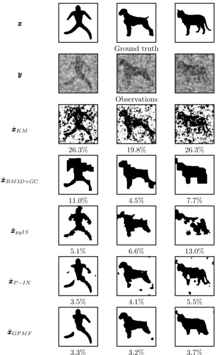
Figure 0.3.: Segmentation non-supervisée de la matière organique. De gauche à droite : le mCT observé, la segmentation par champ de Markov caché classique, la segmentation par le nouveau modèle GPMF. La résolution des artéfacts par le modèle GPMF est bien meilleure, elle réduit le nombre de faux-positifs et faux-négatifs.
Ys
Xs
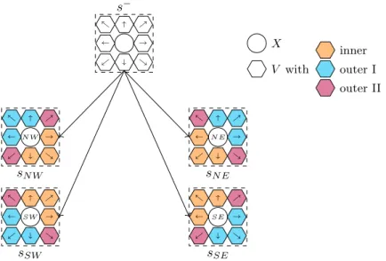
Figure 0.4.: Arbre de Markov caché classique (gauche) et STMT (droite). Les arbres sont de taille 4. Les variables cachées sont en rond, les vari-ables visibles en carré grisé et les varivari-ables auxiliaires en losange. Nous notons les corrélations directes bien plus riches dans le mod-èle STMT où l’inférence reste cependant exacte.
Le modèle Spatial Triplet Markov Tree
Dans cette thèse, nous développons également un nouveau modèle d’arbre de Markov triplet nommé Spatial Triplet Markov Tree (STMT) basé sur ( Cour-bot, Monfrini, et al., 2018). Ce modèle intègre des variables aléatoires auxili-aires afin d’enrichir les possibilités de modélisations. Le modèle STMT est une généralisation des arbres de Markov caché classique.
De plus nous étudions ses liens avec les champs de Markov cachés classiques. Le nouveau modèle semble en effet exhiber des corrélations semblables aux champs mais offre des possibilités d’inférence exacte grâce à la structure d’arbre. Une telle propriété a pour principal avantage d’éviter le recours à des procé-dures itératives souvent approximantes, plus longues et induisant des pertes de précision. Nous étudions les corrélations à l’intérieur du nouveau modèle STMT avec la technique de l’inférence variationnelle à variables aléatoires aux-iliaires. Le modèle STMT est aussi utilisé dans le cadre de la segmentation de calcifications sur des images mCT. La Figure 0.4illustre les modèles d’arbres de Markov.
(a) (b)
Figure 0.5.: Exemples de modèles probabilistes graphiques plus généraux. Gauche : Spatial Bayes Network. Droite : fully-connected Condi-tional Random Field. Les ronds blancs représentent une variable cachée et les carrés gris représentent une variable observée.
Inférence variationnelle dans des modèles plus complexes
Nous étudions des modèles plus généraux dans le sens où plus de dépendances directes sont modélisées entre les variables aléatoires.Pour les modèles graphiques orientés, alors que tous les modèles de Markov cachés classiques sont associés à des graphes ne présentant ni cycles ni semi-cycles, nous proposons un nouveau modèle qui contient des semi-cycles appelé Spatial Bayes Network. La représentation graphique de ce modèle est donnée Figure 3.9. L’introduction de semi-cycles rend l’inférence beaucoup plus com-plexe et nous résolvons ce problème en ayant recours à l’inférence variationnelle. Pour les modèles graphiques non-orientés, il est possible de complexifier le modèle en ajoutant des dépendances conditionnelles entre les variables qui agrandissent les voisinages. Le modèle des fully-connected Conditional Ran-dom Fields est un modèle probabiliste populaire en segmentation d’images qui est associé à un graphe totalement connecté (voir Figure0.5b). Nous étudions à nouveau plusieurs techniques d’inférence variationnelle afin de pouvoir mener l’inférence dans ce modèle.
Segmentation de stents
Dans les images CT, les stents peuvent apparaître fortement déformés à cause des artéfacts qui les entourent. Nous proposons une modélisation basée sur les chaînes de Markov cachées et un modèle de bruit particulier qui permet de segmenter finement le stent dans un environnement complexe (tel que celui de la Figure0.2). Notre approche opère de manière non-supervisée et est entière-ment automatique grâce à l’algorithme d’estimation des paramètres que nous développons également. Une illustrations des résultats de cet algorithme est donnée dans la Figure0.6.
Segmentation histologique tridimensionnelle d’artères
Dans une dernière partie, nous mettons au point un protocole pour la créa-tion de la première base de données d’images annotées d’artères explantées
Figure 0.6.: Segmentation d’un stent explanté par notre approche.
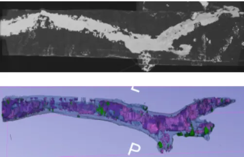
Figure 0.7.: Segmentation tridimensionnelle d’une artère pathologique. Haut : Image rayons-X originale. Bas : Notre segmentation histologique. touchées par l’athérosclérose. Ensuite, nous développons un réseau de neu-rones convolutionnel de type U-Net (Ronneberger et al., 2015) afin de procéder à la segmentation bidimensionnelle histologique des images. L’objectif de ce projet unique est de permettre une première analyse histologique de l’artère uniquement à l’aide du scanner.
Une reconstruction tridimensionnelle propre est obtenue grâce à un post-traitement basé sur une inférence variationnelle dans un modèle de champs aléatoires conditionnels (Krähenbühl and Koltun, 2011). Nous étudions égale-ment une amélioration de cette dernière procédure d’inférence variationnelle utilisant les chaînes de Markov. Un exemple de segmentation tridimensionnelle d’une artère est visible dans la Figure0.7.
Conclusion
Les modèles développés au cours de la thèse apportent des contributions sur des enjeux cruciaux de la modélisation des images par modèles graphiques probabilistes tout en répondant à des problématiques modernes de la chirurgie vasculaire.
Introduction
Advances in vascular surgery and current issues
Cardiovascular Diseases
Cardiovascular Diseases (CVDs) are a major cause of mortality in the world, and particularly in developed countries, with an increasing human and mone-tary cost for societies. In 2016, approximately 17.9 million people died world-wide from CVDs, which represents 31% of all deaths4. In 2015, 49 million
people (9.6% of the population) in the European Union where living with a CVD, the total costs are estimated to e210 billion with e111 billion of direct health care costs and e99 billion indirect costs (productivity loss and informal care of people)5. A major cause of the rise of CVDs is also the increasing
lifetime: this causes new diseases, related to old age, to be seen more widely and needing to be treated. But CVDs are also often linked with life hygiene: smoking, sedentarity and nutrition are habits with direct effects on health in general and more particularly on the cardiovascular system6.
CVDs include a number of heart and blood vessel conditions. Among the most prevalent conditions, one can note ischemic heart disease, stroke and high blood pressure. These conditions often relate to another condition called atherosclerosis. Atherosclerosis is a disease of the arterial wall (not restricted to coronary arteries). It consists in the formation of plaques, called atheromatous plaques, which mostly contain lipids, macrophage cells, connective tissues and calcium (Rafieian-Kopaei et al., 2014). The deposition of calcium contributes to the plaque hardening and the sclerosis of the artery, but it is also what makes the plaque clearly visible on X-ray images. Therefore, one commonly refers to the atheromatous plaques as calcifications since the latter are the most easily identifiable elements of the plaques. Those plaques may grow and/or break which disturbs or, in the most severe cases, stops the blood flow (total occlusion of the artery, rupture of the artery, etc.). These situations are medical emergencies (Rosenfeld, 2000). However, in some cases, atherosclerotic plaques can remain stable and/or regress (Dave et al., 2013). Much is yet to discover about this phenomenon which is summarized in Figure0.8.
In this thesis, our research will be applied to pathologies affecting the arteries of the lower limbs, as well as their surgeries and their treatments, which are described in the next section. More precisely, we will focus on the superficial
4https://www.who.int/en/news-room/fact-sheets/detail/cardiovascular-diseases-(cvds) 5http://www.ehnheart.org/cvd-statistics.html
6https://healthmetrics.heart.org/wp-content/uploads/2017/10/
Figure 0.8.: Summary of the atherosclerotic process. From (CNX, 2016). femoral artery and the popliteal artery which are located in the human body in Figure 0.9. The choice of the femoropopliteal arterial segment was made because it is still the most challenging area for treatment, it is also the most often affected segment in the arterial tree.
Remark: Strictly speaking, cardiovascular refers to the heart and its main arteries and veins. Hence, we will use the adjective vascular to refer to the ar-teries of the lower limb. However, the problematics and pathologies that affect the vessels are identical or very similar.
Remark: Veins will not be mentioned in this thesis since they do no develop atherosclerosis (G. Saul and Gerard, 1991).
Vascular surgery: open and endovascular approaches
Vascular surgery began with the first attempt to control a bleeding vessel. (S. G. Friedman, 2005)The traditional approach in vascular surgery, often called open surgery, relies in opening the patient body up to the affected vessel. The vessel is then repaired or replaced. This approach can lead to high-risk interventions and might not be tolerated by already weak patients such as old patients or patients with a chronic illness. In such cases, the latter have increased chances of complications, including death, following the intervention.
A more recent approach is endovascular surgery, in which new interventions and protocols are regularly created since the last two decades of the 20th
cen-tury. In this interventional technique, the vessel is reached and treated from the inside. With an incision in a peripheral artery, the surgical tools and treat-ments are brought to the desired location, by the inside of the blood vessel, following the patient’s vascular tree. The treatment often includes a biomate-rial. Biomaterials are introduced in the next section.
Figure 0.9.: Arteries of the lower limbs (anterior view). From (CNX, 2016). Endovascular interventions rely heavily on imaging to see inside the patient which is not opened: the terms image-guided surgery and mini-invasive are then often associated with endovascular surgery. This surgical technique is of-ten a solution proposed to patients who cannot undergo open surgery. The risk of medical complications and the patient’s traumatism following an en-dovascular procedure is reduced (Nichols and Wei, 2011). While endovascular techniques have classically been linked with a higher monetary cost than open surgery procedures, the gradually decreasing cost of the treatment and of the patient’s length of stay becomes an additional asset for endovascular proce-dures (Sternbergh III and Money, 2000) (Brinster et al., 2020).
Note that interventional techniques, either from endovascular or open surgery, are constantly improved and updated. A complete reference to endovascular history, techniques and biomaterials is available in (Jing et al., 2018).
Endovascular surgery is a modern approach which raises new questions on biomaterials and new challenges on the per-operative use of imagery during surgical interventions and at all the other stages of the patient’s treatment. Those questions are the motivations behind this thesis.
Biomaterials and related problematics
Biomaterials[A biomaterial is] a systemically and pharmacologically inert sub-stance designed for implantation within or incorporation with living systems. (J. Park and Lakes, 2007)
(a)
(b) (c)
Figure 0.10.: Common biomaterials in vascular surgery: (a) a stent manufac-tured by Cook8, (b) a stentgraft manufactured by Bard9, (c) a
vascular prosthesis manufactured by Gore10.
Biomaterials are found in many medical fields: knee or hip prosthesis in orthopedic surgery, intraocular lens in ocular surgery, heart valve in cardiac surgery, etc. We focus here in biomaterials in vascular surgery. Following (Jing et al., 2018), we list the most common biomaterials:
• Stents are metallic biomaterials widely used to solve problems such as stenosis or dissection of the artery. Once they have been brought to the location of the lesion via the intravascular path, they are released. They are either self-expandable or expanded with a surgical balloon. A stent is illustrated in Figure 0.10a.
• Stentgrafts are distinguished from the (bare) stents described above by the covering (most of the time in polytetrafluoroethylene or polyethy-lene terephthalate7) added over the stent. Stentgrafts are used mainly in
aneurysm repairs or aortic dissections for their capacity to seal the vessel wall. The Figure0.10bdepicts a stentgraft.
• In the most severe cases of lesions, such as complete stenosis or occlusion, the vessel can be replaced with vascular protheses. They may originate from an autogenous vein (the ideal case for biocompatibility) or from an artificial prosthesis which can again be made of PTFE or PET. Note that, as opposed to stents and endografts, an implantation of a vascular prosthesis involves an open-surgery procedure. However they offer better performance and stability than stentgrafts in terms of biocompatibility, fracture resistance and ability to seal the vessel wall. A vascular prosthesis can be seen in Figure0.10c.
To treat a given lesion, the choice of the model and size of the biomaterial depends mainly on the patient’s imaging analysis and the surgeon’s experience.
7Polytetrafluoroethylene (PTFE) and Polyethylene Terephthalate (PET) are
thermoplas-tics. Note that their biocompatibility with the human body is debated (Nabil Chakfé et al., 2020).
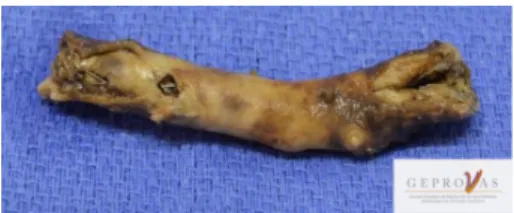
Figure 0.11.: Explanted stent from a superficial femoral artery. The stent itself can be seen, it is encapsulated in a biological material (artery). Remark: In this thesis, we will mainly work with medical images of ex-plants. In vascular surgery, explanting is the act of removing an implanted bio-material or a part of a blood vessel. Note that when a biobio-material is explanted, it is almost always encapsulated in some biological material. An explant can be seen in Figure0.11.
Problematics
Biomaterials in vascular surgery are recent treatments. While these devices benefit from constant improvements and are increasingly implanted, many ques-tions remain unanswered:
• The mechanical behavior of the implanted stents are almost unknown. Simulations, or in vitro experiments, only partially reflect the reality of the constraints applied on a biomaterial implanted in a living body. In vivo mechanical data are still very much ignored and biomaterial man-ufacturers would greatly take advantage of such data. For example, the optimal stent design is still much debated (Raffort et al., 2020).
• The choice of the endovascular procedure is still very dependent on the experience of the surgeon. Objective mathematical tools and databases to guide clinicians are still lacking (Ohana et al., 2014).
• In many cases, the cause(s) of failure of the vascular biomaterials are ignored or unclear. Why did the stentgraft covering tear? Why did the stent fracture? This highlights the need of new analysis tools for explanted biomaterials to investigate biomaterial failures (Chakfé and Heim, 2017) (Lejay et al., 2018).
• Although the whole branch of endovascular surgery relies heavily on im-ages, those medical images remain widely unused. Indeed we could benefit from deeper, large-scale and automated analyses, carried by new tools that researchers in image processing could provide (Raffort et al., 2020). The perspectives of image processing for vascular surgery are the
8https://www.cookmedical.com/products/224e3666-308f-4244-8695-6fd23bbd671c/ 9https://www.crbard.com/Peripheral-Vascular/en-US/Products/
FLUENCY-Plus-Endovascular-Stent-Graft
central motivation for this thesis and are discussed in depth later in this introduction.
We have only listed a small sample of questions arising today in the field of vascular surgery. Yet, addressing these questions already requires joint work from research teams from many fields (biomechanics, image processing, vas-cular surgery, textile sciences, artificial intelligence, histolopathologists, etc.). However, this translational research is also dependent on the availability of data (explanted biomaterials, explanted arteries, patient’s clinical images, patient’s clinical data, antecedents and outcomes, etc.). Since this research involves hu-man subjects on a new topic, the data is scarce and sometimes unavailable due to legal issues. Availability of the data is a crucial point in the field of image processing as we will see later.
The Geprovas laboratory
The Geprovas11 laboratory (Groupe Européen de Recherche sur les Prothèses
liées à la Chirurgie Vasculaire), located in Strasbourg, France, has been founded in 1993 by Professor Nabil Chakfé. It has become a worldwide actor in the field of biomaterials, with an original and unique expertise for devices from vascular surgery. The Geprovas is organized around four activities: the collect and analysis of explants, the innovative research on biomaterials, the medical education program and the clinical analysis program. One of the main goals of Geprovas is to remove barriers and motivate translational research to help answer questions in medical research such as the questions we listed in the previous section.
The work presented in this thesis is initiated and supported by the explant analysis program of the Geprovas. In this context, our work benefited from the wide knowledge of the Geprovas experts as well as from its unique database of explants from vascular surgery.
Medical image processing and new challenges
In the previous section, we mentioned medical imaging and its key role in the modern approaches in vascular surgery. In this second part of the introducion, we present medical imaging in more details. We start with very general defini-tions and gradually shift our focus towards the mathematical methods linked with image analysis studied in this thesis. The goal is to develop approaches which are automated. Automated analysis is indeed the modern way to pro-cess images relying on the power of computers to support medical practice and research.
Medical image processing
Main concepts and vocabularyA bidimensional (respectively tridimensional) image is a set of values arranged on a rectangular (respectively cubic) grid12. For numerical images, the grid is
discretized. If the values are scalars, the image is called grayscale, if the values are vectors, the image is a color image in some color space (Fieguth, 2010).
The most common medical image processing operations are image segmen-tation, which consists in dividing an image into non-overlapping regions with homogeneous properties, image registration, which deals with associating the objects/features in one image with those in one or more other images, and im-age denoising, which aims at estimating a noise-reduced imim-age given an imim-age corrupted by noise (Fieguth, 2010). Image segmentation is the task studied in this thesis and all the methods we develop can be linked with the final goal of segmentation.
A numerical image has to be constructed with some devices, in medical image processing, it is related to the notion of image modality.
Medical imaging modalities
The observed image that we have to process can be of different types in medical research. Those are called the imaging modalities: they are acquired with different devices relying on different physical phenomena to form the image. Thus, the imaging of the same physical object will result in different images with different properties according to the modality. Following (Suetens, 2017), the main medical imaging modalities for diagnosis and treatment13 are now
listed:
• ray Computed Tomography (CT) is an imaging technique based on X-rays. X-rays are electromagnetic waves with wavelengths around 10−10m
which are attenued differently according to the matter it interacts with. The computation of the attenuations undergone by X-rays at certain lo-cations of the space are at the foundation of X-ray images. Computed Tomography (CT) refers to the technique of the computations of the at-tenuations. X-rays have been used in medical imaging starting from the end of the 19thcentury. Figure0.12ashows a typical CT scan image from
vascular surgery.
• Magnetic Resonance Imaging (MRI) is an imaging modality introduced in the medical field in the 1970s. In MRI, the reconstructed image illustrates the magnetic properties of the object of interest. In normal operating conditions, MRI is safer for patients than CT imaging or PET imaging (see next item) because MRI does not rely on ionizing radiations.
12The definition straightforwardly extends to higher dimensions.
13The use of these modalities for medical diagnosis and treatment defines the medical field
• Positron Emission Tomography (PET) is a technique from the field of nuclear medical imaging. It uses a tracer molecule that will be involved in a metabolic process of the body. The tracer molecule is injected to the patient and can be localized because some identified radioactive atoms of the molecule emit γ-rays (wavelength below 10−11m). This way, an
abnormal metabolism can be detected. PET is used clinically since the 2000s.
Note that some modalities describe the anatomy, this is called structural imaging and this is the case for most CT and MRI performed. Others depict a function, this is called functional imaging; PET is a functional imaging modal-ity. In more specific contexts, a modality can be ambivalent and relate to both structural and functional imaging.
In this thesis, we will only develop approaches for X-ray images. Indeed, X-ray images are more common than any other modalities in vascular surgery notably because current MRI devices can be unsafe for patients with a metallic implant. Indeed, MRI might induce stent dislodgement, heating and important image artifacts (Jabehdar Maralani et al., 2020). X-ray images have also the advantage of being a totally non-invasive technique14, the body of the patients
does not need to be touched.
Our work will be more particularly focused on the potential assets of micro-computed tomography (mCT or microCT) X-ray images used for the research in vascular diseases. The formation of mCT images follows the same principles as CT X-ray images described above but they are suited for the imaging of small objects (animals 15, stones, wood, etc.). Notably, mCT modality deals
particularly well with the imaging of explanted arteries. Those images offer a much greater spatial resolution than classic CT scans since pixel sizes are on the scale of the micrometer (Flannery et al., 1987). The first report of a microtomographic image dates back to 1982 in (J. C. Elliott and Dover, 1982). Figure0.12bshows a mCT image of an arterial cross-section.
Remark: We will also mention optical microscopy, which is an image modal-ity that uses light to image a very thin section of an object of interest, which often cannot be analyzed or seen by the naked eyes (Davidson and Abramowitz, 2002). Figure 0.12c describes an arterial cross-section seen in optical mi-croscopy. The work in this thesis will not deal with a direct processing such images, however microscopic images will be essential in the project described in Chapter5.
Main challenges
In this section, we describe the difficulties linked with medical image processing that motivate the approaches we developed during the thesis.
14Provided we tolerate the ionizing radiations which are problematic for some
pa-tients (Pearce et al., 2012) but also clinicians (Brun et al., 2018).
15Some illustrations of the possibilities offered by mCTs in the imaging of small animals are
(a) CT: slice of a CT scan which depicts an abdominal cross-section of a human body. A stent implanted in the aorta is visible at the center of the image. Artifacts are also visible, see Figure0.13for more details.
(b) mCT: cross-section of a stented and explanted superficial femoral artery.
(c) Microscopy: histological cross-section of an explanted, stented and totally occluded superficial femoral artery.
Figure 0.12.: Illustrations of the CT, mCT and microscopy medical imaging modalities with examples from vascular surgery.
(a) CT scan (b) mCT scan
Figure 0.13.: Metallic artifacts in X-ray scans hiding the underlying anatomy. Elements around the stent parts are hardly discernible. Green, red and blue arrows respectively indicate stent metallic artifacts, stent components and calcification components.
Metallic biomaterials and artifacts
We have discussed above that metallic stents (and metallic biomaterials in general) are an issue for MRI scanning but some problems also arise in CT scans. Due to high variations of attenuations in metallic parts according to the X-ray energy level, the CT reconstruction algorithms introduce artifacts in the reconstructed images. The artifacts are problematic since they hide the underlying anatomy. Figure0.13illustrates stent metallic artifacts in vascular X-ray scans. This issue is becoming increasingly important because of the development of biomaterials (orthopedic prostheses, stents, pacemakers, etc.). To answer this problem, many approaches to Metal Artifact Reduction (MAR) have been developed in the literature. See (H. S. Park et al., 2015) for an introduction on stent metallic artifacts and MAR.
Availability of the data
In some medical applications data are scarce while in other fields data abound. This variable then plays a role on the processing approach to follow and on the problem complexity. In vascular surgery, biomaterials were usually destroyed after explantation or patient’s death and relatively little research could be car-ried. As stated earlier, the goal of the explant analysis program of the Geprovas is precisely to collect such data, and make it available in a database that can be used in subsequent studies.
An image analysis task in which no images can be used to learn the algo-rithm parameters, i.e., where the algoalgo-rithm has to work with the observed image alone, is called unsupervised. In the opposite case, it is called a super-vised task. Both approaches will be seen in the thesis. Note that a supervised problem requires a human interaction at some stage, for example, to add an-notations to the data.
Remark: Collections of biological samples used for scientific investigation, or biobanks, are initiatives that are slowly gaining popularity (PW Scholtes et al., 2011).
Computational costs
Image processing can rapidly become a computationally intensive task, espe-cially for medical images. We encounter this problem in our work dealing with mCT images which are big, high resolution images. In other problematics, when a database with hundreds of elements must be processed, the treatments must be wisely chosen. In this thesis, some of the works study the problem of computational complexity.
Remark: Our developments are however not constrained by speed consid-erations. Our primary data are images of explanted materials, thus the time constraint is not comparable at all to developments linked with videos or real-time analyses such as (Nwoye et al., 2019).
Image processing and probabilistic modeling
In this thesis, the main contributions will be focused on probabilistic graphical models applied to image segmentation, particularly Hidden Markov Models (HMM) (Baum and Petrie, 1966) and their extensions to Pairwise and Triplet Markov Models (Pieczynski and Tebbache, 2000) (Lanchantin et al., 2011) (Gorynin, Gangloff, et al., 2018). Markovian models offer a simple and intuitive way to introduce dependencies between the pixels of the images and thus, they can be a relevant answer to the problematics previously presented.
For example, it will be seen that stent metallic artifacts (illustrated in Fig-ure 0.13) can be modeled by spatially correlated noise: a pixel value at a location is highly dependent on the neighboring pixel values. Such a noise is naturally taken into account in Pairwise and Triplet Markov Models. Such correlations are also studied in models based on Gaussian Markov Random Field (Rue and Held, 2005) (GMRF). In this thesis, these models are then studied as possible improvements to MAR algorithms and as a way to perform segmentation in images degraded with spatially correlated noise.
A second asset to probabilistic models is that they are relatively efficient in unsupervised problems. Following the popular Expectation Maximization ( Demp-ster et al., 1977) (EM) algorithm, there is a rich literature of learning algorithms in unsupervised context for graphical models (Celeux et al., 1995) (Tieleman, 2008). They are then competitive methods for problems with scarce and/or missing data.
Probabilistic models also benefit from a very active research community fo-cusing on optimization methods. Efficient approaches exist to approximate computations that cannot be done exactly. See for example (C. Zhang et al., 2018) which deals with Variational Inference (VI). They also offer much mod-elization power with possibly auxiliary random variables (Lanchantin et al.,
2011) and can then fit many complex real life problems (Courbot, Monfrini, et al., 2018).
Probabilistic graphical models will be introduced in depth in Chapter1.
Outline of the thesis
This thesis is composed of five chapters and their appendices.
Chapter 1 consists in a literature review of the main concepts and devel-opments around probabilistic modeling with graphical models with a special focus on image segmentation. This chapter sets up all the definitions and no-tations that will be used more in depth in subsequent chapters. Chapters 2,
3 and 4present the core research of this thesis dealing with the improvement and development of new probabilistic models for image segmentation. Chap-ter2proposes a new model of Markov Fields, called Gaussian Pairwise Markov Fields (GPMF), for the unsupervised segmentation of regions that are corrupted with long-spatially correlated noise. The model is tested on both artificial and real datasets. Chapter 3 describes a new model of Markov Trees, called Spa-tial Triplet Markov Tree (STMT), aiming at being a deterministic counterpart to Markov Fields, which are also used in the context of unsupervised image segmentation. Theoretical results and applications on real data are provided. STMTs make use of auxiliary random variables, the enhanced correlations they introduce are largely studied. Chapter4 proposes a review on Deep Learning for medical imaging and describes the development of a Convolutional Neural Network for semantic segmentation. This segmentation is subsequently im-proved by a new approximate inference approach for a model of Conditional Random Fields that is also presented in Chapter 4. Chapter 5 illustrates the applications to vascular surgery of the probabilistic graphical models developed along the thesis.
The appendix of each chapter gives the full details of calculations and addi-tional observations.
List of publications
During this thesis, several journal and conferences articles have been written. They are listed below according to the part of the thesis they deal with. For completeness, the other publications from the author of the thesis are also listed even if their topic is not directly related to the content of this thesis.
First we list the publications primarily directed to the signal processing com-munity:
• Chapter 2:
– Under review: Unsupervised Segmentation with Gaussian Pair-wise Markov Fields, H. Gangloff, J.-B. Courbot, E. Monfrini, C. Collet, Computational Statistics & Data Analysis, 2020.
– (Gangloff, Courbot, et al., 2019): Segmentation non-supervisée dans les champs de Markov couples gaussiens, H. Gangloff, J.-B. Courbot, E. Monfrini, C. Collet, Colloque GRETSI, 2019.
• Chapter 3:
– Under review: Unsupervised Image Segmentation with Spatial Triplet Markov Trees, H. Gangloff, J.-B. Courbot, E. Monfrini, C. Collet, International Conference on Acoustics, Speech, and Signal Processing, 2021.
– (Gangloff, Courbot, et al., 2020): Spatial Triplet Markov Trees for auxiliary variational inference in Spatial Bayes Networks, H. Gan-gloff, J.-B. Courbot, E. Monfrini, C. Collet, Stochastic Modeling Techniques and Data Analysis, 2020.
• Chapter 4:
– Under review: Markov Chain Variational Inference in Fully-Connected Conditional Random Fields, H. Gangloff, E. Monfrini, C. Collet, In-ternational Conference on Acoustics, Speech, and Signal Processing, 2021.
• Chapter 5:
– (Gangloff, Monfrini, Collet, et al., 2020): Unsupervised segmenta-tion of stents corrupted by artifacts in medical X-ray images, H. Gangloff, E. Monfrini, C. Collet, N. Chakfé, International Confer-ence on Image Processing Theory, Tools and Applications, 2020. – (Gangloff, Monfrini, Collet, et al., 2019): Segmentation de stents
dans des données médicales à rayons-X corrompues par les artéfacts, H. Gangloff, E. Monfrini, C. Collet, N. Chakfe, Colloque GRETSI, 2019.
• Not in the thesis:
– (Gorynin, Crelier, et al., 2016): Performance comparison across hid-den, pairwise and triplet Markov models’ estimators, I. Gorynin, L. Crelier, H. Gangloff, E. Monfrini, W. Pieczynski, International Conference on Applied and Computational Mathematics, 2016. – (Gorynin, Gangloff, et al., 2018): Assessing the segmentation
perfor-mance of pairwise and triplet Markov models, I. Gorynin, H. Gan-gloff, E. Monfrini, W. Pieczynski, Signal Processing, 2018.
– (Gangloff, Monfrini, Ghariani, et al., 2020): Improved Centerline Tracking for new descriptors of atherosclerotic aortas, H. Gangloff, E. Monfrini, M.Z. Ghariani, M. Ohana, C. Collet, N. Chakfé, Inter-national Conference on Image Processing Theory, Tools and Appli-cations, 2020.
We then present the publications primarily directed to the vascular surgery community:
• Chapter 5:
– (Kuntz et al., 2020): Co-registration of peripheral atherosclerotic plaques assessed by conventional CT-angiography, micro-CT and histology in CLTI patients, S. Kuntz, H. Jinnouchi, M. Kutyna, S. Torii, A. Cornelissen, Y. Sato, M. E. Romero, F. Kolodgie, A. V. Finn, A. Schwein, M. Ohana, H. Gangloff, A. Lejay, N. Chakfé, R. Virmani, European Journal of Vascular & Endovascular Surgery, 2020.
– Under review: Automated histological segmentation on micro-computed tomography images of atherosclerotic arteries, S. Kuntz*, H. Gangloff*, H. Naamoune, E. Monfrini, C. Collet, A. Lejay, M. Kutyna, R. Virmani, N. Chakfé, European Journal of Vascular & Endovascular Surgery, 2020.
Chapter 1.
Main concepts in probabilistic
modeling
Contents
1.1. Introduction . . . 24
1.2. Graphical modeling. . . 24
1.2.1. Main definitions . . . 24
1.2.2. Directed Graphical Models . . . 25
1.2.3. Undirected Graphical Models . . . 27
1.3. Inference in probabilistic models . . . 28
1.3.1. Exact inference . . . 29
1.3.2. Approximate inference . . . 30
1.4. Parameter estimation . . . 30
1.4.1. Maximum Likelihood estimation . . . 31
1.4.2. Estimation for DGMs . . . 31
1.4.3. Parameter estimation for UGMs . . . 32
1.5. Probabilistic models for image segmentation. . . 33
1.5.1. Definitions and context . . . 33
1.5.2. Bayesian image segmentation . . . 34
1.5.3. Discriminative and generative models . . . 35
1.6. Hidden Markov Models . . . 35
1.6.1. Main families of HMMs . . . 36
1.6.2. Pairwise and Triplet extensions . . . 39
1.1. Introduction
This chapter introduces probabilistic modeling with a focus on Hidden Markov Models and on applications to probabilistic image segmentation. More in-depth introductions can be found in popular books on the topic such as (C. M. Bishop, 2006) (Goodfellow et al., 2016) (Koller and N. Friedman, 2009) (Murphy, 2012) (Wainwright and Michael I Jordan, 2008).
1.2. Graphical modeling
1.2.1. Main definitions
Elements of graph theoryA graph G = (S, E) is formed by a set of vertices S, that we also refer to as sites or nodes, and by a set of edges E. We have E ⊂ S × S, since, in general, not all vertices are connected by an edge. The set of vertices connected to a vertice s ∈ G is called the neighborhood of s and is denoted Ns. Note that we have
s /∈ Ns. A clique is a subset of S with the property that every two elements are
connected by an edge. A clique is then a fully-connected subset. A maximal clique of G is clique of G which cannot accept any more vertice from G without breaking the clique property. A tree is a connected graph without any cycle. In a graph G, the edges can either be directed, undirected or a mix of both. This leads to different families of probabilistic models which we discuss in the next sections. In the graphical representation of the probabilistic graphical models we will use arrows to represent directed edges. The absence of arrow represents an undirected edge. These first definitions are illustrated in Figure1.1.
In a probabilistic graphical model, each vertice s of G is associated with a random variable whose name then contains the name of the vertice as subscript, for example, Xs. a b c d e f g h i An undirected graph S = {a, b, c, d, e, f, g, h, i} c = {a, b, d, e}is a clique The subset c is fully connected Ne= {a, b, c, d, f, g, h, i}
Na= {b, d, e}
Figure 1.1.: Examples and notations of graph theory I. Elements of probability theory
Let X be a random variable from a probability to space, equipped with a probability measure p, to a measurable space (E, E). If E is a finite or countable set, then X is said to be a discrete random variable. If E is an uncountable
1.2. Graphical modeling set, then X is said to be a continuous random variable. In both cases, we are interested in measuring the probability of X taking certain values, i.e., we want to evaluate the quantities of the type PX(A) = p(X ∈ A), ∀A ∈ E. Such
computations involve PX another probability measure. PX is called the law of
X which is more precisely called distribution in the discrete case and density in the continuous case. The definitions are similar for random vectors. When considering the law of random vectors made of both continuous and discrete random variables, we may use indistinctly the term distribution or density. If PX is the law of a random variable X, we may write X ∼ PX.
If X is a discrete random variable, we denote by x its realization, ∀x ∈ E. When A is a singleton, i.e., A = x, ∀A ∈ E, we have p(X ∈ A) = p({X = x}). When there is no ambiguity we write p({X = x}) = p(X = x) or even p({X = x}) = p(x)1 to denote the probability of a realization x of X. Similarly, if X is a continuous random variable, in case of no ambiguity, we might use p(x) to refer to the density of X. If X ∼ PX, we denote the expectation of X by E[X],
which can also be written, with a slight notation abuse, Ex∼p(x)[x].
The conditioning of a probability law on the realization of some other random variable(s) will be written classically with a vertical bar |. For example, using the notation shortcuts mentioned above, the law of X given the realization y of random variable Y will be written p(x|y).
All our definitions extend to the multivariate case: random variables then become random vectors. Some of the random vectors we will work with are more precisely stochastic processes. However, stochastic processes and their properties are out of the scope of this thesis and little will be said about them.
1.2.2. Directed Graphical Models
Directed Graphical Models (DGMs), also known as Beliefs Networks, have di-rected edges represented by an arrow between two vertices. Let (s, s0) ∈ S2,
if there is a directed edge from s to s0 then s is called the father node of s0,
conversely, s0 is called the child node of s. A node s may have several fathers,
which are refered to as the set of parents of s, denoted P(s). A node for which the parent set is empty is refered to as a root node. Furthermore we denote ¯S the set of vertices which have at least one father. Figure1.2illustrates the new notions we have just introduced.
The notion of Directed Acyclic Graph (DAG), also known as Bayesian Net-works, refers to graphs where all the edges are directed and where the graphs do not contain directed cycles. The directed edges of a DGM leads to a partial ordering of its vertices (Wainwright and Michael I Jordan, 2008). A directed tree is a DAG which does not contain any directed cycles and not any semi cycles. A semi cycle is the DAG that has been obtained after reversing some arrow directions of a directed cycle.
In this thesis we will focus on several kinds of directed rooted trees, called arborescences. In such graphs the root vertice is unique, it is then the only
1Note that this last notation shortcut then confuses p with P
X but no ambiguity is raised
a c d e g h A directed graph S = {a, c, d, e, g, h} ¯ S = {d, e, g, h}
aand c are root nodes ais the father of d dis the son of a P(d) = {a, e, g}
{d, g, h}forms a directed cycle Figure 1.2.: Examples and notations of graph theory II.
a c d e g h A DAG {d, g, h} is a semi cycle a c d e g h A directed tree a d e g h An arborescence a b c d A directed chain
Figure 1.3.: Examples and notations of graph theory III.
vertice with no edge pointing towards it, and all the other edges are directed away from it. Note that in arborescences, the fact that there is only one root node implies that all the other non-root nodes have exactly one father. When all the vertices of an arborescence have one son (except for the last vertice), we obtain a directed chain. Figure 1.3 shows examples of the newly defined graphs.
DGMs are specified by local conditional probabilities which are given for ev-ery random variables associated to evev-ery site: ∀s ∈ S the associated conditional probability is p(xs|xxxxxxxP(s)). If r is a root node, the associated conditional
prob-ability is p(xr). The joint probability distribution defining a DGM is obtained,
using the definition of conditional probabilities, by multiplying the local con-ditional probabilities: p(xs1, xs2, . . . , xsN) = Y r∈S\ ¯S p(xr) Y s∈S p(xs|xxxxxxxP(s)), (1.1)
where s1, . . . , sN are the N vertices of S.
Sampling in a DGM is performed by ancestral sampling: starting from the root nodes we follow the partial order over the nodes, and we sample each time the associated random variable using the local conditional probability (Goodfellow et al., 2016).
1.2. Graphical modeling Conditional independence of random variables given other random variables (or Markov property) is an important property when dealing with graphical models. The procedure of d-separation can determine whether there is condi-tional independence (Murphy, 2012). A particular result of this procedure that will be underlying many of our studies is for arborescences: let A, B and C be subsets of S. ∀a ∈ A, ∀c ∈ C, the random variables {Xa}a∈Aand {Xc}c∈C are
said to be conditionally independent given B if every path (without considering the direction of the edges) between a and c goes through a vertice from B.
1.2.3. Undirected Graphical Models
Undirected Graphical Models (UGMs), also known as Markov Random Fields (MRFs), have undirected edges. They are defined differently from DGMs. We call potential functions, or factors or unnormalized probability distributions, a real non-negative function φC({xs}s∈C) = φC(xxxxxxxC) associated with a clique
C. Potential functions describe the interactions between random variables. We then have that an UGM is defined by a set of random variables XXXXXXXwhich admits for joint distribution:
p(xxxxxxx) = 1 Z
Y
C∈C
φC(xxxxxxxC), (1.2)
where C is the set of all cliques of G and Z is the partition function or normal-ization constant, defined as:
Z =X x x x x x x x Y C∈C φC(xxxxxxxC). (1.3)
The partition function ensures that the distribution sums to 1. As a special parametrization, a probability distribution which takes the form of Equation1.4
is known as a Gibbs distribution: p(xxxxxxx) = 1 Zexp (−E(xxxxxxx)/T ) = 1 Z exp − 1 T X C∈C ψC(xxxxxxxC) ! (1.4) where E is called the energy function, ψC are some potential functions and T
is a parameter called the temperature (with T > 0). All the MRFs seen in this thesis will follow a Gibbs distribution.
An equivalent definition for UGMs is possible due to the Hammersley-Clifford theorem (Hammersley and Peter, 1971). A set of random variables XXXXXXX, defined such that: (
p(xxxxxxx) > 0, for all set of realizations XXXXXXX = xxxxxxx, p(xs|xxxxxxxS\{s}) = p(xs|xNs), ∀s ∈ S,
(1.5) forms an UGM or MRF, with respect to the neighborhood N . The MRF defini-tion of Equadefini-tion1.5is called the full conditional definition. The Hammersley-Clifford theorem proves that the definitions of Equations1.4and1.5are equiv-alent. It then appears that the conditional independence property (Markov property) for UGMs is simpler than for DGMs. A random variable at site s,
given the realizations of the random variables located in its neighborhood Ns, is
conditionally independent from all the remaining random variables (i.e., from all the vertices in S \ Ns).
Sampling realizations from UGMs is not as straightforward as for DGMs. Except from few exceptions where sampling can be done without approxima-tions (Stoehr, 2017), Markov Chain Monte Carlo (MCMC) approaches are the most popular way for this task. The Gibbs sampler is a widely used algorithm to sample from UGMs. It belongs to the MCMC approaches and is a special case of the Metropolis-Hastings algorithm (S. Geman and D. Geman, 1984). The Gibbs sampler relies on the full conditional probabilities and generates a Markov chain of samples which is proved to converge to the joint distribution. The Gibbs sampler is interesting when samples from the joint distribution can-not be directly drawn, as it is the case in general. The algorithm is given in AlgorithmA.1.
Extensions of the Gibbs sampler algorithm are an active research topic, no-table examples are the chromatic Gibbs sampler (Gonzalez et al., 2011) or the blocked Gibbs sampler (Brown et al., 2019). Another extension for the Gibbs sampler consists in improving the exploration of the modes of the joint distribution using tempered transitions (Salakhutdinov, 2009). Lastly, in the particular case of Gaussian Markov Random Fields studied in Chapter2, sam-pling can be done in a single iteration of a fully-blocked Gibbs sampler or a single sampling from a standard normal distribution followed by Fourier-based transformations (Rue and Held, 2005).
Remark: The notions of trees and chains also exist for UGMs, they will not be mentioned in this chapter for brevity.
Remark: In practice, many models, such as those studied in this thesis, have both directed and undirected edges. In such cases, the associated proba-bility distribution, the parameter estimation process and the inference process for these mixed models will straightforwardly follow either from the DGM the-ory or UGM thethe-ory.
Remark: Note that Factor Graphs (Frey, 2003) are a popular kind of graphi-cal models that aims at unifying UGMs and DGMs. Factor Graphs are however out of the scope of this thesis.
1.3. Inference in probabilistic models
Inference in a probabilistic model can refer to several closely related computa-tional tasks:
• Computing a marginal distribution p(xxxxxxxA), A ⊂ S.
• Computing a conditional distribution p(xxxxxxxA|xxxxxxxB), A ⊂ S, B ⊂ S and A 6=