HAL Id: cel-00392215
https://cel.archives-ouvertes.fr/cel-00392215
Submitted on 5 Jun 2009
HAL is a multi-disciplinary open access archive for the deposit and dissemination of sci-entific research documents, whether they are pub-lished or not. The documents may come from teaching and research institutions in France or abroad, or from public or private research centers.
L’archive ouverte pluridisciplinaire HAL, est destinée au dépôt et à la diffusion de documents scientifiques de niveau recherche, publiés ou non, émanant des établissements d’enseignement et de recherche français ou étrangers, des laboratoires publics ou privés.
DifferentialEquations in Finance
Jacques Printems
To cite this version:
Jacques Printems. Notes on Numerical Methods for Partial DifferentialEquations in Finance. 3rd cycle. Hanoi (Vietnam), 2007, pp.59. �cel-00392215�
Equations in Finance
Jacques Printems
Universit´e de Paris 12e-mail: [email protected]
http://perso-math.univ-mlv.fr/users/printems.jacques/
Summer School of Mathematical Finance CIMPA – IMAMIS – VIETNAM
Institute of Mathematics 18 Hoang Quoc Viet Road
10307 HANOI 23/4 – 4/5/2007
Contents
1 PDE in Mathematical Finance 5
1.1 Black-Sholes analysis . . . 5
2 Finite Difference Methods for PDE 9 2.1 Introduction . . . 9
2.1.1 Taylor’s expansion: a formal framework . . . 9
2.1.2 Forward Finite Difference for the first derivative . . . 10
2.1.3 Backward Finite Difference for the first derivative . . . 10
2.1.4 Centered Finite Difference for the first derivative . . . 11
2.1.5 FD approximations for the second derivative . . . 11
2.1.6 FD approximations in dimension 2 . . . 12
2.2 Short study of the heat equation. Stability and precision . . . 14
2.3 General parabolic case . . . 21
2.4 Numerical computation of options in dimension 1 . . . 22
2.4.1 European case . . . 22
2.5 Numerical computation in dimension 2 . . . 23
2.5.1 European case . . . 26
3 Finite Elements Methods for PDE 29 3.1 Toy model 1: Dirichlet problem . . . 29
3.2 Abstract framework and discretization . . . 30
3.3 Toy model 2: Obstacle problem . . . 32
3.4 Numerical implementation of options in dimension 1 . . . 34
3.4.1 The European case . . . 35
3.4.2 The American case : projected Gradient method . . . 36
3.4.3 Some numerical results . . . 37
4 Asian options 41
Partial Differential Equations in
Mathematical Finance
1.1
Black-Sholes analysis
The purpose of theses notes is to introduce some numerical tools based on P.D.E. for the pricing of one of the most popular derivative products based on equities, i.e. the options. Most of this introduction is taken from [8] (chapter 3).
The simplest financial option, a European call option, is a contract with the following conditions:
• At a prescribed time in the future, known as the expiry date, the owner of the option may
• purchase a prescribed asset, known as the underlying asset or, briefly, the under-lying, for a
• prescribed amount, known as the exercise price or strike price.
The word may in this description implies that for the owner (the holder) of the option, this contract is a right and not an obligation. One of our main concerns throughout theses notes is to find:
• How much would one pay for this right ?
The option to buy an asset as described above is known as a call option. The right to sell an asset is known as a put option.
Let us derive now the original Black & Scholes partial differential equation for the price of the simplest options, so-called vanilla options. Let us introduce some simple notation.
• We denote by V the value of an option; V is a function of the current value of the underlying asset, S, and time, t: V = V (S, t). The value of the option also depends on the following parameters:
• σ, the volatility of the underlying asset;
• K the exercise price; • T , the expiry or maturity; • r the interest rate.
First we consider what happens just at the moment of expiry of a call option, i.e. at time t = T .
If S > K at expiry, it makes financial sense to exercise the call option, which cost an amount K to obtain an asset worth S. The profit os such a transaction is S − K. On the other hand, if S < K at expiry, we should not exercise the option because we would make a loss of E − S > 0. In this case, the option expires valueless. Thus, the value of the call option at expiry can be written as
V (S, T ) = max(S − K, 0).
More generally, suppose that we have an option whose value V (S, t) depends only on S and t (regardless whether V is a call or a put). Let us also suppose that the asset price S follows the lognormal random walk
dS
S = µ dt + σ dB, (1.1.1)
where B is a Wiener process. Using Itˆo’s lemma, we can write
dV = ∂ V ∂t dt + ∂V ∂S dS + 1 2σ 2S2∂2V ∂S2 dt (1.1.2) = µ ∂ V ∂t + µS ∂ V ∂S + 1 2σ 2S2∂2V ∂S2 ¶ dt + σS∂ V ∂S dB.
This is the random walk followed by V . Note that such an equation need V to be regular enough.
Let us now consider a portfolio Π which contains the option and a ratio −∆S of the asset S the option is based on, namely
Π = V − ∆S. (1.1.3)
Using (1.1.1) and (1.1.2) together gives the random walk followed by Π: dΠ = dV − ∆dS, = µ ∂ V ∂t + µS ∂ V ∂S + 1 2σ 2S2∂2V ∂S2 − µ∆S ¶ dt + σS µ ∂ V ∂S − ∆ ¶ dB,
where we have used the self-financed feature of the portfolio, i.e. d(∆)S = 0 (it means that ∆ is held fixed during the time-step dt).
We can then eliminate the random component in this random walk by choosing
∆ = ∂V ∂S. (1.1.4)
This result in a portfolio whose increment is now deterministic dΠ = µ ∂ V ∂t + 1 2σ 2S2∂2V ∂S2 ¶ dt. (1.1.5)
The concepts of arbitrage and supply and demand tell us that the right hand side of (1.1.5) must be equal to rΠ dt. Thus, we have
rΠ dt = µ ∂ V ∂t + 1 2σ 2S2∂2V ∂S2 ¶ dt. (1.1.6)
Then substituting (1.1.3) and (1.1.4) into (1.1.6) leads to ∂ V ∂t + 1 2σ 2S2∂2V ∂S2 + rS ∂V ∂S − rV = 0. (1.1.7)
Finite Difference Methods for PDE
2.1
Introduction
2.1.1 Taylor’s expansion: a formal framework
The Finite Difference (FD) method is based on the properties of the Taylor’s expansion and on the application of the definition of derivatives. It is the simplest method when the mesh is uniform but it needs the mesh to be regular enough. Indeed, in dimension n, the nodes of the mesh are located at the intersection of n families of curves, each of them belonging to a unique curve of each family.
Its purpose is to approximate differentials equations. Indeed, it allows to construct approximations of the derivative operator D = ∂x∂ acting on differentiable functions of the real variable x.
Following [5], we can present shortly the method in dimension 1 in a (very) formal framework. Let us consider a spatial discretization
−∞ < · · · < xi−1< xi< xi+1< · · · < +∞,
which is regular in the sense that xi+1− xi = ∆x is supposed to be constant. Let v a function regular
enough on R (let say v ∈ C∞
b ). We set for any i ∈ Z, vi= v(xi) and we introduce the operators
Evi = vi+1, (2.1.1) δ+ vi = vi+1− vi, δ−vi = vi− vi−1, δvi = vi+1/2− vi−1/2, ¯ δvi = (vi+1− vi−1)/2, µvi = (vi+1/2+ vi−1/2)/2,
where we noted vi±1/2= v(xi±1/2) with xi+1/2= (xi+1− xi)/2.
Let D be the derivative operator on the functions : Dv(x) = ∂ v
∂x(x). The FD method essentially exploits the Taylor formula in a way which can be summarized like that:
vi+1= vi+ ∆xDv(xi) +∆x 2 2 D 2 v(xi) +∆x 3 3! D 3 v(xi) + · · · +∆x n n! D nv(x i) + · · · ,
which allows to write
Evi= exp(∆x D)vi, and E = exp(∆x D).
We will prefer this formulation :
D = 1 ∆xln(E). (2.1.2)
2.1.2 Forward Finite Difference for the first derivative
The formula (2.1.2) allows to express D in function of δ+:
D = 1 ∆xln(1 + δ +) (2.1.3) = 1 ∆x ∞ X k=1 (−1)k+1(δ +)k k , = 1 ∆x µ δ+−(δ +)2 2 + (δ+)3 3 + · · · 
Of course, this expansion should be restricted to analytic functions. For polynomial functions, the right member of the expansion has only a finite number of terms. Since δ+ = O(∆x), the truncated expansion with n + 1 first terms yields an approximation O(∆xn) of D. This gives:
Dvi = vi+1− vi ∆x − ∆x 2 vxx(xi) + · · · (2.1.4) = vi+1− vi ∆x + O(∆x) Dvi = −3vi+ 4vi+1− vi+2 2∆x + ∆x2 3 vxxx(xi) + · · · (2.1.5) = −3vi+ 4vi+1− vi+2 2∆x + O(∆x 2)
(useful for the approximation of the derivative at the frontier of a domain)
2.1.3 Backward Finite Difference for the first derivative
Again (2.1.2) and (2.1.1) yield to:
D = − 1 ∆xln(1 − δ −) (2.1.6) D = 1 ∆x µ δ−+(δ −)2 2 + (δ−)3 3 + · · · ¶ .
The formulæ are of the same kind: Dvi= vi− vi−1 ∆x + O(∆x) (2.1.7) Dvi = 3vi− 4vi−1+ vi−2 2∆x + O(∆x 2) (2.1.8)
2.1.4 Centered Finite Difference for the first derivative
In a first time, we write D with respect to δ. It comes
δ = 2 sinh µ ∆xD 2 ¶ , and then D = 2 ∆xargsinh µ δ 2 ¶ = 2 ∆xln à δ 2 + r 1 +δ 2 4 ! , or D = 2 ∆x à δ 2 − 1 6 µ δ 2 ¶3 + 3 40 µ δ 2 ¶5 − 5 112 µ δ 2 ¶7 + · · · ! . (2.1.9)
Nevertheless, this formula gives an expression of D with respect to the value of v at the middle of the mesh and not at the nodes. In order to obtain an expression in function of ¯
δ, we use the following relation between µ and δ:
µ2 = 1 +δ
2
4 , which can be easily derived from the relations (2.1.1).
Multiplying (2.1.9) by the relation 1 = µ(1 + δ2/4)−1/2, we obtain
D = 1 ∆xµ µ δ − 1 6δ 3+ 1 30δ 5− 1 140δ 7+ 1 630δ 9· · ·¶. (2.1.10) Finally µδ = ¯δ gives: Dvi = ui+1− ui−1 2∆x − ∆x2 6 uxxx+ · · · Dvi =
ui−2− 8ui−1+ 8ui+1− ui+2
12∆x +
∆x4
30 u5x+ · · · and so on.
2.1.5 FD approximations for the second derivative
We end this subsection by FD schemes for D2. Such approximations can be derived from Eqs (2.1.3), (2.1.6) and (2.1.9) squared.
• First order forward FD :
D2vi=
vi+2− 2vi+1+ vi
∆x2 + O(∆x)
• First order backward FD :
D2vi= vi− 2vi−1+ vi−2
∆x2 + O(∆x)
• Second order centered FD : D2vi =
vi+1− 2vi+ vi−1
∆x2 + O(∆x
2)
2.1.6 FD approximations in dimension 2
Let v be a regular enough function of the variables x and y. We focuse here on the approximation of the second deriviative of v with respect to x, y: ∂
2v ∂x2, ∂2v ∂y2 and ∂2v ∂x∂y. Approximations of the first two is simply the corresponding approximation of the second derivative of v(·, y) viewed as a function of x or v(x, ·) viewed as a function of y.
Particular attention has to be paid for the the mixed derivative. A first try leads to the second order approximation:
µ ∂2u ∂x∂y ¶ i,j = 1
∆x∆yδ¯xδ¯yui,j+ O(∆x
2, ∆y2),
(2.1.12)
with obvious notations. This is represented by the following figure 2.1
1
1
−1
−1
Figure 2.1: Representation of formula (2.1.12).
Other consistant examples (i.e. approximation of order greater or equal to one) are µ ∂2u ∂x∂y ¶ i,j = 1 ∆x∆yδ¯xδ +
yui,j+ O(∆x2, ∆y),
(2.1.13) µ ∂2u ∂x∂y ¶ i,j = 1 ∆x∆yδ +
xδy+ui,j+ O(∆x, ∆y),
(2.1.14) µ ∂2u ∂x∂y ¶ i,j = 1 ∆x∆yδ −
xδy−ui,j+ O(∆x, ∆y),
(2.1.15)
whose representations are in Fig.2.2. The truncature errors in the last two approximations (2.1.14) and (2.1.15) are of opposed sign, it means that the arithmetic mean will be second order approximation in both x and y:
µ ∂2u ∂x∂y ¶ i,j = 1 2∆x∆y ¡
δx+δ+y + δx−δ−y¢ui,j+ O(∆x2, ∆y2).
(2.1.16)
The same is also true for µ ∂2u ∂x∂y ¶ i,j = 1 2∆x∆y ¡
δx+δ−y + δx−δ+y¢ui,j+ O(∆x2, ∆y2).
Figure 2.2: Representation of formulæ (2.1.13)–(2.1.15).
−2
1
−1
−1
1
1
1
2
−1
−1
1
−1
−1
1
More generally, every convex linear combinaison of the last two approximations leads to a second order approximation. We will see that (2.1.17)–(2.1.16) are stable approximation of the mixed derivative whereas (2.1.12) is not.
2.2
Short study of the heat equation. Stability and precision
In order to illustrate the basic concepts of numerical analysis, such as stability and accuracy, in the framework of finite difference methods, we will consider the heat equation. Let us recall that the Black & Scholes PDE under suitable change of varaibles can be transformed into the heat equation.
Let α > 0. We consider the following PDE: ∂ u
∂t(x, t) = α ∂2u
∂x2(x, t), (x, t) ∈] − L, L[×]0, T [,
(2.2.18)
with the following boundary and initial conditions:
u(x, 0) = h(x), x ∈] − L, L[, (2.2.19)
and
u(−L, t) = l1(t), u(L, t) = l2(t), t ∈]0, T [.
(2.2.20)
Computation domain : cartesian grid xi = i∆x, tn= n∆t for 1 ≤ i ≤ M and 0 ≤ n ≤ N
with
∆t = T /N, ∆x = 2L/(M + 1), for N et M two integer ≥ 1.
The operator ∂
2
∂x2 is approached by (2.1.11) at the points xi∈] − L, L[ by
∂2u
∂x2(xi, tn) = α
u(xi+1, tn) − 2u(xi, tn) + u(xi−1, tn)
∆x2 + O(∆x
2)
(2.2.21)
As regards the time integrator, we use a so-called θ-scheme which can be found from (2.1.4) and (2.1.5) applied to u(xi, t) at time t = tn (resp. at time t = tn+1) and a convex linear
combinaison: u(xi, tn+1) − u(xi, tn) ∆t = θ ∂ u ∂t(xi, tn+1) + (1 − θ) ∂ u ∂t(xi, tn) + O(∆t), (2.2.22) = θα∂ 2u ∂x2(xi, tn+1) + (1 − θ)α ∂2u ∂x2(xi, tn) + O(∆t), where θ ∈ [0, 1].
When θ = 0, we recover the Explicit Euler-scheme, θ = 1, the Implicit Euler Scheme and when θ = 1/2, the Crank–Nicolson scheme. Let us note that in the case where θ = 1/2, the truncation errors in (2.1.4) and (2.1.5) are opposite, so that the term in ∆ vanishes and we recover a second order scheme in time. Any other choice of θ leads a first order scheme in time.
We replace u(xi, tn) par uni et O by 0 and then (2.2.21)–(2.2.22) gives the following
system of difference equations:
(Σ) un+1i − uni ∆t = αθ ∆x2 ¡ un+1i+1 − 2un+1i + un+1i−1¢+α(1 − θ) ∆x2 ¡ uni+1− 2uni + uni−1¢, 1 ≤ i ≤ M, 0 ≤ n ≤ N.
We define now the consistancy error of the scheme Σ.
Definition 2.2.1 We call consistance error the remaining terms when you replace uni in the scheme by the exact solution u(xi, tn), denoted by εni.
Eqs (2.2.21)–(2.2.22) leads easily to the bound
|εni| ≤ C³∆tβ + ∆x2´, (2.2.23)
where C depends on the higher order derivatives of u with respect to x and t and where β = 1 si θ 6= 1/2 and β = 2 otherwise.
Let us make now an important remark which is at the center of Numerical Analysis : the smallness of εni gives us a clue about the degree of approximation of the equation, not about the approximation of the unknown u. We will say that (Σ) is consistant iif εni tends to 0 when ∆t, ∆x tend to 0. So a scheme is consistant when it approximates the equation.
Before going further, let us use the matrix notation. We set Un = un1 .. . un M ∈ RM.
Then the scheme (Σ) can be written as µ I + αθ ∆t ∆x2L ¶ Un+1= µ I − α(1 − θ) ∆t ∆x2L ¶ Un+ ∆tFn, (2.2.24) where L = 2 −1 0 · · · 0 −1 . .. ... ... ... 0 . .. ... ... 0 .. . . .. ... ... −1 0 · · · 0 −1 2 ∈ RM ×M and Fn= αθ∆x∆t2l1(tn+1) + α(1 − θ)∆x∆t2l1(tn) 0 .. . 0 αθ∆x∆t2l2tn+1) + α(1 − θ)∆x∆t2l2(tn) ∈ RM.
Eq. (2.2.24) can be written under the following ”integrated” form :
Un= AnθU0+ ∆t n−1 X k=0 An−k−1θ µ I + αθ ∆t ∆x2L ¶−1 Fk, (2.2.25) with U0= u(x1, 0) .. . u(xM, 0)
(e.g.), and where
Aθ = µ I + αθ ∆t ∆x2L ¶−1µ I − α(1 − θ) ∆t ∆x2L ¶ .
Eq. (2.2.25) suggests that at each time step, one has to inverse a linear system (except when θ = 0). We do not precise in theses notes the way we are doing that. Let us say that we can use in the context of the heat equation in dimension 1, the Gauss elimination algorithm without encounter any problems (as storage, efficiency, . . . ).
We are going to show now that the scheme (Σ) is convergent in some sense, i.e. that uni tends to u(xi, tn) in some sense when ∆t and ∆x tend to 0. We can imagine that the
smallness of εn
i is not sufficient for that. Indeed, the formulation (2.2.25) says that the
consistancy errors are accumulating in time in order to form the global error. We need one more assumption : the stability.
Hypothesis 1 Let us suppose that Aθ is such that
kAθk2≤ 1.
(2.2.26)
We have denoted by kBk2, for a matrix B, the operator norm based on the Euclidean norm
in RM. It means that
kBk2 = sup x∈RM, kxk2=1
kBxk2.
We will say that the scheme is L2-stable if A
θ satisfy the assumption (2.2.26). We can
now state :
Proposition 2.2.2 Under the assumption (2.2.26), (Σ) is convergent in the sense where
lim N,M −→+∞0≤n≤Nmax ∆x M X i=1 |u(xi, tn) − uni|2 = 0. Proof We set eUn= u(x1, tn) .. . u(xM, tn)
, En= Un− eUn, the vector of the (global) errors et En=t[εn1, . . . , εnM] the
consistancy error (or local errors) at time tn.
Due to the definition 2.2.1 of the local errors, we have directly: µ I + αθ ∆t ∆x2L ¶ En+1= µ I − α(1 − θ)∆x∆t2L ¶ En+ ∆t En. (2.2.27)
The stability criterion (2.2.26) allows us to bound the global error at time tnsince we can control the
accumulation of the local errors. Indeed, the time integrated version of (2.2.27), i.e. (2.2.25) where Un
replaced by En and Fn replaced by Enyields
kEnk2≤ kE 0 k + ∆t n−1 X k=0 ° ° ° ° ° µ I + αθ ∆t ∆x2L ¶−1°° ° ° °kE k k. (2.2.28)
We show now that the operator norm in the last inequality can be majorized by 1. Let Y ∈ RM and let us
consider X ∈ RM such that µ
1 + αθ ∆t ∆x2L
¶ X = Y.
It is sufficient to show that kXk2≤ kY k2. Indeed, taking the scalar product of the last equality by X, leads
to
kXk22+ αθ
∆t
We note now that L is a positive (even definite positive) operator. Indeed, (LX, X) = M X i=1 (2zi− zi−1− zi+1) zi = M X i=1 (zi+1− zi)2+ z21+ z 2
M (by discrete integration by part),
where we set z0= zM +1= 0. We conclude by the Cauchy-Schwarz inequality.
Now (2.2.28) is reduced to kEnk2≤ kE 0 k + ∆t n−1X k=0 kEkk. (2.2.29) Plugging (2.2.23) in (2.2.29) yields kEnk2≤ C∆t n−1 X k=0 √ M (∆tβ+ ∆x2) ≤ CT√M (∆tβ+ ∆x2),
which is the desired result since√M ≤ ∆x−1/2.
Remark 2.2.3 We have shown the convergence in the functional space L∞(0, T, L2(R)).
Indeed, we note the analogy between
max 0≤n≤N∆x M X i=1 |eni|2 and sup t∈[0,T ] Z L 0 |e(x, t)|2dx.
What are now the conditions on the parameters (α, θ and especially ∆t and ∆x) under which Σ is L2-stable ? We can answer by the following spectral study. In fact,
the eigenvectors and eigenvalues of L can be found to be (using trigonometric formulæ for example) Xk= sin³M +1kπ ´ .. . sin³M +1M kπ´ , λk = 4 sin 2 µ kπ 2(M + 1) ¶ , 1 ≤ k ≤ M.
So the eigenvalue of Aθ are
µk=
1 − 4α(1 − θ) sin2³2(M +1)kπ ´ 1 + 4αθ sin2³2(M +1)kπ ´
, 1 ≤ k ≤ M.
It is easy to verify that the function ψ : t 7→ (1 − 4α(1 − θ)∆t/∆x2t)/(1 + 4αθ∆t/∆x2t) is
non increasing on [0, 1]. Moreover, ψ(1) = (1 − 4α(1 − θ)∆t/∆x2)/(1 + 4αθ∆t/∆x2). Now
we note that ψ(0) = 1. In order to have |ψ(t)| ≤ 1 and hence |µk| ≤ 1 for any k, we have
to show that ψ(1) ≥ −1. This gives us the L2-stability criterion:
α(1 − 2θ) ∆t ∆x2 ≤
1 2. (2.2.30)
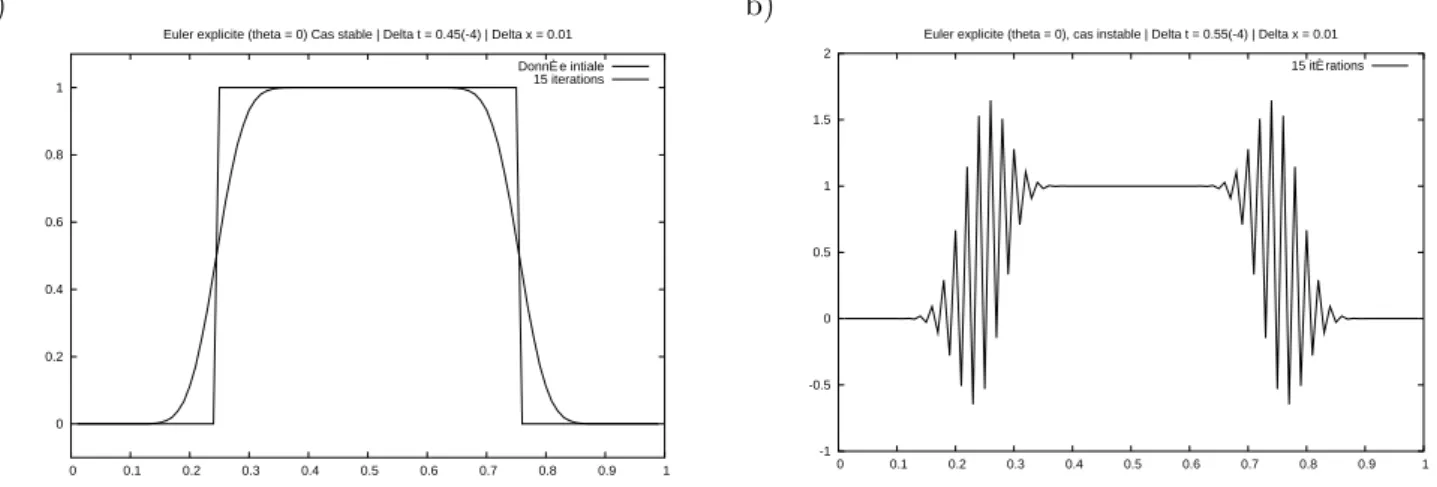
We are going now to numerically test whetever these conditions of stability (and hence of convergence) are ”sharp” or not in the case θ = 0 (Explicit Euler scheme). In order to do that we choose α = 1 a piecewise constant initial condition h on [0, 1] :
h(x) = u(x, 0) = ½
1 si x ∈ [0.25, 0.75] 0 sinon.
Let us fix ∆x = 0.01. The stability criterion (2.2.30) gives a theoretical limit for the time step: ∆t = 0.5 × 10⁻⁴.
The following scilab script simulate the scheme (Σ) with a time discretization just below and just beyond the theoretical limit. We can see in Fig 2.4 that the condition (2.2.30) have to be satisfied and is a necessary condition when θ = 0.
// Discretization parameters M=99; N=22000; // Stable case //N=18000; // Instable case nmax=15; // Parameters alpha=1; theta=0;
// Do not edit below
L=2*diag(ones(M,1))-diag(ones(M-1,1),-1)-diag(ones(M-1,1),1); I=eye(M,M);
Deltat=1/N; Deltax=1/(M+1);
A=inv(I + alpha*theta*Deltat/Deltax^2*L)*(I - (1-theta)*alpha*Deltat/Deltax^2*L); // Initialisation of U^n x=linspace(0,1,M+2); y=1*((x>=0.25)&(x<=0.75)); U=y(2:100)’; // time iteration for i=1:nmax, U=A*U; end xbasc(); plot(x(2:100),U)
Before the end of this paragraph, let us mention another important notion of stability : the L∞-stability. We will say that the scheme (Σ) is L∞-stable iff
kAθk∞≤ 1,
(2.2.31)
where we have used here the notation kBk∞, for a matrix B, for the operator norm based
on the supremum norm in RM. It means that
kBk∞= sup
x∈RM, kxk∞=1
kBxk∞, where kxk∞= max 1≤i≤M|xi|.
a) 0 0.2 0.4 0.6 0.8 1 0 0.1 0.2 0.3 0.4 0.5 0.6 0.7 0.8 0.9 1 Euler explicite (theta = 0) Cas stable | Delta t = 0.45(-4) | Delta x = 0.01
DonnØe intiale 15 iterations b) -1 -0.5 0 0.5 1 1.5 2 0 0.1 0.2 0.3 0.4 0.5 0.6 0.7 0.8 0.9 1 Euler explicite (theta = 0), cas instable | Delta t = 0.55(-4) | Delta x = 0.01
15 itØrations
Figure 2.4: Excplit Euler scheme (θ = 0) after 15 iterations in time for α = 1, M = 99, N = 22000 a), N = 18000 b).
What are the conditions on the parameters under which the scheme is L∞-stable ? And does it converge in this case ?
Proposition 2.2.4 Let ∆t > 0 and ∆x > 0 such that 2α(1 − θ) ∆t
∆x2 ≤ 1.
(2.2.32)
Then the scheme (Σ) is L∞-stable and moreover it converges in the following sense:
lim
N,M −→+∞0≤n≤Nmax 1≤i≤Mmax |u(xi, tn) − u n i| = 0.
Proof
First let us prove stability. Let X ∈ RM, kXk
∞= 1 and Y = AθX. We have µ I − α(1 − θ)∆x∆t2L ¶ X = µ I + αθ ∆t ∆x2L ¶ Y, or, for any 1 ≤ i ≤ M,
µ 1 − 2α(1 − θ)∆x∆t2 ¶ zi+ α(1 − θ) ∆t ∆x2(zi+1+ zi−1) = µ 1 + 2αθ ∆t ∆x2 ¶ yi− αθ ∆t ∆x2(yi+1+ yi−1), (2.2.33)
where we have set z0= zM +1= y0= yM +1= 0.
Let i0, j0 be the indices such that yi0= max1≤i≤Myiand yj0= min1≤j≤Myj. The system of equations
(2.2.33) imply yi0 ≤ zi0+ 2α(1 − θ) ∆t ∆x2(1 − zi0), yj0 ≥ zj0+ 2α(1 − θ) ∆t ∆x2(−1 − zj0).
Thus a sufficient condition of stability is (2.2.32). Morevover, if we consider Ineq. (2.2.28) where k · k2 is
replaced by k · k∞, then we will have convergence of the scheme in the same techniques than in Proposition
done this. In fact, let us consider again X and Y with kXk∞= 1 and X = (I + αθ∆t/∆x2L)Y . The same
ideas as above can by applied here and we get
yi0≤ zi0 ≤ 1, and yj0 ≥ zj0≥ −1,
with the same notations. Hence kY k∞≤ 1.
We sum up in the table 2.1 the sufficient conditions of stability of θ–schemes applied to the heat equation.
Table 2.1: Sufficient conditions of L2 and L∞-stability of θ–schemes.
θ–schemes L∞ L2
θ = 0 2α∆t ≤ ∆x2 2α∆t ≤ ∆x2
θ = 0.5 α∆t ≤ ∆x2 no conditions
θ = 1 no conditions no conditions θ ∈ [0, 1] 2α(1 − θ)∆t ≤ ∆x2 2(1 − 2θ)∆t ≤ ∆x2
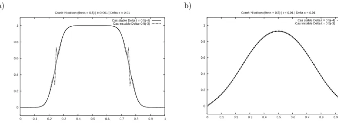
We will now test the stability conditions in the case of the Crank–Nicolson scheme (θ = 1/2). We set ∆x = 0.01 (M = 99 points). The critical value of ∆t is 10−4. Figure 2.5 (a) shows the result obtained at time t = 0.001 in the two cases (stable and instable) and (b) at time t = 0.01. We can see that the differences vanishes with time.
We have used the previous scilab script.
a) 0 0.2 0.4 0.6 0.8 1 0 0.1 0.2 0.3 0.4 0.5 0.6 0.7 0.8 0.9 1 Crank-Nicolson (theta = 0.5) | t=0.001 | Delta x = 0.01
Cas stable Delta t = 0.5(-4) Cas instable Delta=0.5(-3)
b) 0 0.2 0.4 0.6 0.8 1 0 0.1 0.2 0.3 0.4 0.5 0.6 0.7 0.8 0.9 Crank-Nicolson (theta = 0.5) | t = 0.01 | Delta x = 0.01
Cas stable Delta t = 0.5(-4) Cas instable Delta t = 0.5(-3)
Figure 2.5: Crank–Nicolson scheme (θ = 0.5) for α = 1 and N = 99. a) t = 0.001 : the dash line represent the instable case (∆t = 0.5 × 10⁻³) and the solid line, the stable case (∆t = 0.5 × 10⁻⁴). Same notations for b) at time t = 0.01.
2.3
General parabolic case
One can easliy see that results of stability of the previous section can be generalized to the case where the discrete Laplacian −L is replaced by a matrix B such that the following
holds: bi,i≤ 0, bi,j ≥ 0, i 6= j, M X j=1 bi,j = 0. (2.3.34)
The scheme (Σ) can be written in this case as µ I − αθ ∆t ∆x2B ¶ Un+1= µ I + α(1 − θ) ∆t ∆x2B ¶ Un+ ∆tFn.
What are the new L∞-stability criterion ? With the same notation than in the previous section, we have yi0−αθ ∆t ∆x2bi0,i0yi0−αθ ∆t ∆x2 X j6=i0 bi0,jyj = xi0+α(1−θ) ∆t ∆x2bi0,i0xi0+α(1−θ) ∆t ∆x2 X j6=i0 bi0,jxj.
The conditions [M ] implies that the left member of the previous equation is bounded by below by yi0. Same techniques apply and give as stability’s criterion:
α max
1≤i≤M|bi,i|(1 − θ)
∆t ∆x2 ≤ 1.
(2.3.35)
More generally, if X =t[z1, . . . , zM] ∈ RM and Y = AθX then the same computations as
above give yi0 ≤ xi0 + α(1 − θ) ∆t ∆x2|bi0,i0| µ max 1≤i≤Mxi− xi0 ¶ . Condition (2.3.35) leads to min
1≤i≤Mxi≤ yi≤ max1≤i≤Mxi.
It is the discrete maximum principle. If we replace (2.3.34) by bi,i ≤ 0, bi,j ≥ 0, i 6= j, M X j=1 bi,j ≤ −λ < 0, (2.3.36)
where λ > 0, then B satisfies the strong discrete maximum principle: BX ≥ 0 ⇒ X ≤ 0.
Remark 2.3.1 There are other properties satisfied by the matrices such that (2.3.36) holds: if B satisfies (2.3.36) then B is inversible and B−1 has positive coefficients.
We can sum up this section by saying that (2.3.34) (or (2.3.36)) and (2.3.35) are the two stability criterion in the case of L∞-stability. The first is spatial and the second one is temporal. From now on, we will try to be in this case when we will discretize Black & Scholes type PDE.
2.4
Numerical computation of options in dimension 1
2.4.1 European case
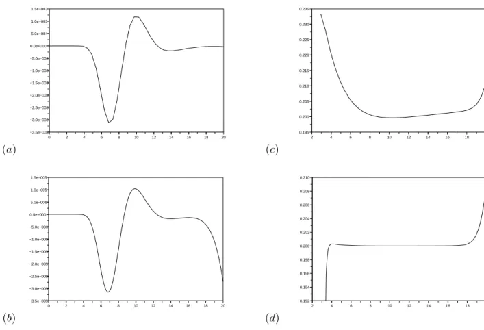
We test our FD scheme on the pricing of a European Put (cf. appendix A.1.) with r = 0.1, σ = 0.2, K = 1 and T = 1. The inversion of the linear system are done by means of standart direct methods which can be found in scilab software (e.g.) (see [4] for a complete reference of the subject of linear system inversion).
We can see below different effect of discretization on the error with respect to the real price (computed owing to Black & Scholes formula) and on the implied volatilities computed thanks to a Newton algorithm (see Appendix A for a Scilab script).
(a) 0 2 4 6 8 10 12 14 16 18 20 −3.5e−003 −3.0e−003 −2.5e−003 −2.0e−003 −1.5e−003 −1.0e−003 −5.0e−004 0.0e+000 5.0e−004 1.0e−003 1.5e−003 (c) 2 4 6 8 10 12 14 16 18 20 0.195 0.200 0.205 0.210 0.215 0.220 0.225 0.230 0.235 (b) 0 2 4 6 8 10 12 14 16 18 20 −3.5e−005 −3.0e−005 −2.5e−005 −2.0e−005 −1.5e−005 −1.0e−005 −5.0e−006 0.0e+000 5.0e−006 1.0e−005 1.5e−005 (d) 2 4 6 8 10 12 14 16 18 20 0.192 0.194 0.196 0.198 0.200 0.202 0.204 0.206 0.208 0.210
Figure 2.6: Different spatial discretization (∆t = 1e − 2). (a), (c) ∆x = 0.5. (b), (d) ∆x = 0.05. Curves (c) and (d) described in both cases the implicit volatility as a function of the spot.
2.5
Numerical computation in dimension 2
We will consider for the sake of simplicity the following two dimensional model of assets: dSi
Si
= µidt + σidBi, i = 1, 2,
where again the parameter µi and σi are supposed to be constant and where B1 and B2
are two Brownian motion whose correlation is denoted by ρ ∈] − 1, 1[. It means that there exists fB2 independant from B1 such that
B2 = ρB1+
p
1 − ρ2Bf 2.
Suppose that we are given an option whose value V (S1, S2, t) depends only on t and S1
and S2. Using the same technique than in section 1.1 (the same delta-hedging strategy), it
is easy to show that V is solution whose PDE can be written ∂V ∂t + 1 2σ 2 1x2 ∂2V ∂x2 + 1 2σ 2 2y2 ∂2V ∂y2 + ρxyσ1σ2 ∂2V ∂x∂y + r(x ∂V ∂x + y ∂ V ∂y) − rV = 0, where r > 0 is the interest rate and where (x, y) ∈ R+ and t ∈ (0, T ). We will consider
the time changed version of this equation (t → T − t) and will discretize it using finite differences. Le us set ∆x = L1 M1+ 1 , ∆y = L2 M2+ 1 , ∆t = T N.
Here M1 and M2 are such that we have exactly M1× M2 points strictly inside the
compu-tation domain (cf. figure 2.7).
(xi, yj) = (i∆x, j∆y), (i, j) ∈ {2, . . . , M1+ 1} × {2, . . . , M2+ 1}.
u(xi, yj, tn) −→ uni,j ∂2u ∂x2(xi, yj, tn) −→ 1 ∆x2(u n
i+1,j − 2uni,j+ uni−1,j)
∂2u
∂y2(xi, yj, tn) −→
1 ∆y2(u
n
i,j+1− 2uni,j+ uni,j−1)
∂2u
∂x∂y(xi, yj, tn) −→ 1 ∆x∆y
¡
2uni,j+ uni−1,j+1+ uni+1,j−1− ui,j+1n − uni,j−1− uni+1,j− uni−1,j¢) Choice for the first order operator:
(Cx) ∂ u ∂x(xi, yj, tn) = 1 2∆x(u n i+1,j − uni−1,j) (D+x) ∂ u ∂x(xi, yj, tn) = 1 ∆x(u n i+1,j − uni,j) (D− x) ∂ u ∂x(xi, yj, tn) = 1 ∆x(u n i,j− uni−1,j)
With the same notations for the derivatives with respect to y. Numerotation of the nodes:
We choose here to integrate the outer nodes (nodes that are on the frontier) in the global numerotation of the unknowns.
1 2 3 5 6 7 8 9 18 10 28 19 4 11 17 36 27 43 44 38 45 37 Figure 2.7: M1= 7, M2= 3
More precisely the unknowns {un
i,j}1≤i≤M1+2,1≤j≤M2+2are represented by a vector U
n= t[Un
1, . . . , U(Mn 1+2)(M2+2)] where
Ukn= uni,j ⇐⇒ k = (M1+ 2)(j − 1) + i.
(2.5.37)
Time scheme : θ-scheme, θ ∈ [0, 1]. Un+1− Un
∆t = (1 − θ)BU
n+ θBUn+1.
The matrix B has a “block structure” (which is typical). Its computation and storage will be done in two independant steps: a matrix Bintfor the inner nodes (which represent the PDE)
and a matrix Bext for the outer nodes (which take into account the boundary conditions).
Let us start with Bint. The storage of Bint are done following the local description of the
finite differences used: ∂2 ∂x2 ∂2 ∂x∂y ∂2 ∂y2 −2 1 1 1 −1 −1 1 2 −1 −1 −2 1 1 ∂ ∂x ∂ ∂y 1/2 −1/2 1/2 −1/2
The step from local numerotation to global one are done using: k+M1+1 k−M1−3 k−M1−2 k−M1−1 k+M1+2 k+M1+3 k k−1 k+1
We are doing a loop (i,j) over the inner nodes of the mesh. We compute the correspond number k thanks to (2.5.37). This number corresponds to the number of the line of the matrix we compute. Non vanishing term of the matrix are hence placed and computed thanks to the coefficients of the local grids. Sparse storage is done using special functions of scilab1. Hence, we have computed Bint.
Now, we will add line in the matrix in order to take into account the boundary condi-tions. Lines will be different depending on what boundary conditions we use. Let k be a number corresponding to an outer points (ex: 9,18,27,36 and 45 on Fig. 2.7).
• Dirichlet boundary condition : Suppose that the value of u is set at the node k, then the line k contains 1 on the diagonal and zero everywhere else.
• Neumann condition : Suppose that the value of ∂ u
∂n has to be set at this node. For example, ∂ u
∂y = 0. Then the line k contains 1/∆y and −1/∆y at the appropriate nodes.
Hence, we have computed a matrix Bext.
The reader can refer to Appendix A.2 where a scilab script compute the two matrices. We give an example of the matrix which discretize the operator ∂x∂y∂2 for M1 = M2 = 2
: ! 0. 0. 0. 0. 0. 0. 0. 0. 0. 0. 0. 0. 0. 0. 0. 0. ! ! 0. 0. 0. 0. 0. 0. 0. 0. 0. 0. 0. 0. 0. 0. 0. 0. ! ! 0. 0. 0. 0. 0. 0. 0. 0. 0. 0. 0. 0. 0. 0. 0. 0. ! ! 0. 0. 0. 0. 0. 0. 0. 0. 0. 0. 0. 0. 0. 0. 0. 0. ! ! 0. 0. 0. 0. 0. 0. 0. 0. 0. 0. 0. 0. 0. 0. 0. 0. ! ! 0. - 1. 1. 0. - 1. 2. - 1. 0. 1. - 1. 0. 0. 0. 0. 0. 0. ! ! 0. 0. - 1. 1. 0. - 1. 2. - 1. 0. 1. - 1. 0. 0. 0. 0. 0. ! ! 0. 0. 0. 0. 0. 0. 0. 0. 0. 0. 0. 0. 0. 0. 0. 0. ! ! 0. 0. 0. 0. 0. 0. 0. 0. 0. 0. 0. 0. 0. 0. 0. 0. ! ! 0. 0. 0. 0. 0. - 1. 1. 0. - 1. 2. - 1. 0. 1. - 1. 0. 0. ! ! 0. 0. 0. 0. 0. 0. - 1. 1. 0. - 1. 2. - 1. 0. 1. - 1. 0. ! ! 0. 0. 0. 0. 0. 0. 0. 0. 0. 0. 0. 0. 0. 0. 0. 0. ! ! 0. 0. 0. 0. 0. 0. 0. 0. 0. 0. 0. 0. 0. 0. 0. 0. ! ! 0. 0. 0. 0. 0. 0. 0. 0. 0. 0. 0. 0. 0. 0. 0. 0. ! ! 0. 0. 0. 0. 0. 0. 0. 0. 0. 0. 0. 0. 0. 0. 0. 0. ! ! 0. 0. 0. 0. 0. 0. 0. 0. 0. 0. 0. 0. 0. 0. 0. 0. ! 1
Only 4 lines has non nul element : it corresponds to the inner points of the domain. Example of matrix Bext with the same data:
-->full(Bext) ans = ! 1. 0. 0. 0. 0. 0. 0. 0. 0. 0. 0. 0. 0. 0. 0. 0. ! ! 0. - 1. 0. 0. 0. 1. 0. 0. 0. 0. 0. 0. 0. 0. 0. 0. ! ! 0. 0. - 1. 0. 0. 0. 1. 0. 0. 0. 0. 0. 0. 0. 0. 0. ! ! 0. 0. - 1. 1. 0. 0. 0. 0. 0. 0. 0. 0. 0. 0. 0. 0. ! ! 0. 0. 0. 0. 1. 0. 0. 0. 0. 0. 0. 0. 0. 0. 0. 0. ! ! 0. 0. 0. 0. 0. 0. 0. 0. 0. 0. 0. 0. 0. 0. 0. 0. ! ! 0. 0. 0. 0. 0. 0. 0. 0. 0. 0. 0. 0. 0. 0. 0. 0. ! ! 0. 0. 0. 0. 0. 0. - 1. 1. 0. 0. 0. 0. 0. 0. 0. 0. ! ! 0. 0. 0. 0. 0. 0. 0. 0. 1. 0. 0. 0. 0. 0. 0. 0. ! ! 0. 0. 0. 0. 0. 0. 0. 0. 0. 0. 0. 0. 0. 0. 0. 0. ! ! 0. 0. 0. 0. 0. 0. 0. 0. 0. 0. 0. 0. 0. 0. 0. 0. ! ! 0. 0. 0. 0. 0. 0. 0. 0. 0. 0. - 1. 1. 0. 0. 0. 0. ! ! 0. 0. 0. 0. 0. 0. 0. 0. 0. 0. 0. 0. 1. 0. 0. 0. ! ! 0. 0. 0. 0. 0. 0. 0. 0. 0. - 1. 0. 0. 0. 1. 0. 0. ! ! 0. 0. 0. 0. 0. 0. 0. 0. 0. 0. - 1. 0. 0. 0. 1. 0. ! ! 0. 0. 0. 0. 0. 0. 0. 0. 0. 0. 0. 0. 0. 0. - 1. 1. !
The linear system can be written in a first step:
(Iint− θ∆tBint)Un+1= Fint,
with
Fint= (Iint+ (1 − θ)∆tBint)Un.
But written like that, there are more unknowns (number of columns = total number of points) than equations (number of line = number of inner points where is written the equation). We complete the system in
(Iint− θ∆tBint+ Bext)Un+1= Fint+ Fext,
where Fext contains the values of u or its derivatives that are to be set for the outer nodes.
2.5.1 European case
We are now going to compute the price of an European Put over the minimum of two assets. Here the payoff function h(S1, S2) = (K − min(S1, S2))+. We use the scilab script in
Appendix A.2. We show in Fig. 2.8 the solution V at time T = 1 as a function of S1and S2.
Parameters of the models has been set to r = 0.1, σ1 = σ2 = 0.2, K = 10 = S1(0) = S2(0),
0 1 2 3 4 5 6 7 8 9 10 Z 0 4 8 12 16 20 X 0 2 4 6 8 10 12 14 16 18 20 Y
Figure 2.8: Value of the Put over the minimum of two assets in a 2d Black & Scholes model. Here, parameters are r = 0.1, σi= 0.2, ρ = 0.5, K = 10 = S1(0) = S2(0) and T = 1.
Finite Elements Methods for PDE
References about Finite Element Methods: [1], [7] for the fundamentals. A good introduc-tion: [3].3.1
Toy model 1: Dirichlet problem
Let be f be a continuous function on (−1, 1). We are faced to three problems: to find the solution u of each of the three following cases.
(D)
u twice differentiable such that −u′′(x) = f (x), for any x ∈ (−1, 1),
with the boundary conditions u(−1) = u(1) = 0.
(V) u ∈ E (u′, v′) = (f, v), for any v ∈ E, (M) u ∈ E
infv∈EF (v) = F (u),
where we have set
E = {v : (−1, 1) → R | v(−1) = v(1) = 0, v, v′ continue and piecewise continue}, and where (f, g) denotes the scalar product in L2(−1, 1) the space of squared integrable
functions on (−1, 1), i.e. (f, g) = Z 1 −1 f (x)g(x) dx, and where F (v) = Z 1 −1 |v(x)|2dx − Z 1 −1 f (x)v(x) dx = 1 2(v ′, v′) − (f, v) for any v ∈ E.
Theorem 3.1.1 Under suitable regularity assumptions on the solution u, the problems (D), (V) and (M) are equivalent.
Proof
We can first show that (D) and (V) are equivalent. Indeed starting from (D), multiplying the differential equation by v ∈ E and integrating by part leads to (V). Conversely, starting from (V), if we know moreover that u is twice differentiable (in fact we can demonstrate this : it is a regularizing property) then we can do the IPP in the other sense.
Let us now show that (M) implies (V). Let u be such that (M) holds. By definition, the function g(ε) = F (u + εv) has a minimum in ε = 0. By calculus, g is differentiable and g′(0) = (u′, v′) − (f, v). Hence g′(0) = 0. Conversely, let u be such that (V) hold and let v ∈ E. We set w = v − u or v = u + w. Expanding the term F (v) = F (u + w) leads to
F (v) = 1 2(u ′, u′) + (u′, w′) +1 2(w ′, w′) − (f, u) − (f, w) = F (u) + (u′, w′) − (f, w) +1 2(w ′, w′) = F (u) +1 2(w ′, w′)
where we have used that E is a linear space, i.e. w = v − u ∈ E and hence satisfies (V). Finally, since (w′, w′) ≥ 0, we can conclude.
We are making now some important remarks. The problem (V) is called the variational formulation of the differential problem (D). Getting from (V) to (D) required regularity results about the solution and also the fact that
Z 1
−1
(u′′+ f ) v dx = 0 ∀v ∈ E implies u′′+ f = 0.
Saying it differently, it means that the space E must be “larger enough”.
Giving a variational formulation relies here on the construction of the space E. We are no more looking after approximated values of the solution at some nodes (as we do in Finite Difference Methods) but we search a function as an element (i.e. a point) belonging to some functional space. It is the main feature of the Finite Element Method that we will briefly describe hereafter.
In order to go further, we will change a bit the functional framework and give a more general setting. Indeed, when f is no more enough regular (let say continuous), the space E is not large enough with respect to the topology induced by the L2 norm on (−1, 1). Thus
we have to deal with its completion: an Hilbert space.
3.2
Abstract framework and discretization
Let V be a real Hilbert space whose scalar product is denoted by (·, ·) and its norm by k · kV. Let a : V × V → R be a blilinear symmetric continue V -elliptic form on V . It means
that the following holds:
(i) a(u, v) = a(v, u) for any u and v in V ;
(iii) There exists M > 0 such that |a(u, v)| ≤ M kukVkvkV for any (u, v) ∈ V2;
(iv) There exists α > 0 such that a(u, u) ≥ αkuk2V, for any u ∈ V .
We call V -ellipticity the last assumption. Let L : V → R be a continuous linear form on V . It means that
(i) |L(v)| ≤ Λkvk for any u in V ;
(ii) L(λu + µv) = λL(u) + µL(v) for any λ, µ ∈ R and (u, v) ∈ V2. Following the beginning of the previous section, we set two problems
(V)
u ∈ V
a(u, v) = L(v), for any v ∈ V,
(M) u ∈ V infv∈V F (v) = F (u), where F (v) = 1
2a(v, v) − L(v) for any v ∈ V .
It is not difficult to see that we recover the previous section’s framework by setting V = H1
0(−1, 1) = {v, v′ ∈ L2(−1, 1), v(−1) = v(1) = 0} and a(u, v) =
R1
−1u′(x)v′(x) dx. In
this case the V -ellipticity on a relies on the Poincar´e Lemma.
We have the following result whose proof relies deeply on the Hilbert structure of the functional space V (Lax-Milgram Theorem):
Theorem 3.2.1 Problems (V) and (M) are equivalent and there exists an unique solution u for these two problems. Moreover, we have
kukV ≤ Λ
α.
Let now discretize the problem (V). Let h > 0 and let Vh be a finite dimensional
subspace of V (we say that the approximation is V -conform) such that dim(Vh) tends to
infinity when h tends to 0. To be specific, we set
Vh= span(ϕ1, . . . , ϕM).
The problem (V) is replaced by
(Vh)
uh=PMi=1uiϕi
a(uh, ϕj) = L(ϕj), for any j ∈ {1, . . . , M }.
It gives a linear system
AU = b,
Theorem 3.2.2 A is positive definite. There exists an unique solution uh ∈ Vh and
kuhkV ≤
Λ α.
This is a stability result. Hence, a Finite Element Method is stable in this case as soon as soon the continuous problem is elliptic. Note that it is not necessarly the case for Finite Different Methods.
We study now the error between u and uh. Indeed, we have
Theorem 3.2.3 For any vh ∈ Vh, we have
ku − uhkV ≤
M
α ku − vhkV. Proof
First, since a is in the two formulation (V) and (Vh), we have by substraction:
a(u − uh, vh) = 0 for any vh ∈ Vh.
We can do that because the approximation is V -conform (vh ∈ Vh⊂ V ). We see that u−uh
is orthogonal to Vh with respect to the scalar product a.
Now, the result relies on the relation a(u − uh, u − uh) = a(u − uh, u − vh+ vh− uh) =
a(u − uh, u − vh) since vh− wh ∈ Vh. We conclude by continuity of a (assertion (iii)) and
V -ellipticity (assertion (iv)).
This last result is fundamental. It says that the error ku − uhkV can be controlled by
any other approximation vh of u in Vh, its interpolant for example. Something which do
not depend on the original problem but only on the space Vhand the way it “approaches”
V .
3.3
Toy model 2: Obstacle problem
As we have seen in the introduction, the problem of the valuation of an American option is very similar with a free boundary problem for the associated Black & Scholes PDE. Indeed, the domain R+× (0, T ) can be separated in two region, the first where one should exercise the option and the case where one should hold the option. Nevertheless, any frontier cannot be chosen. In fact, we can show that at each time t there exists an unique asset price, called the optimal exercise price which divide R+ (i.e. the S-axis) into these two regions. Moreover, V (S, t) must be greater than the payoff function otherwise arbitrage possibilities can occur.
In the case of the American put option, one can show that at each time t, we must divide the S axis into two regions: one where one should exercise and
V = K − S, ∂ V ∂t + 1 2σ 2S2∂2V ∂S2 + rS ∂V ∂S − rV < 0,
(since r > 0) and the other where V (S, t) satisfies locally the Black & Scholes PDE
V > K − S, ∂ V ∂t + 1 2σ 2S2∂2V ∂S2 + rS ∂V ∂S − rV = 0.
We will discuss in this section about a canonical version of this problem: the obstacle problem. The main simplifications are that the problem will be time independant and the PDE will be reduced to the second derivative in space. We will see that this can be written in another form: a variational inequality. We will see that this new formulation is particularly well suited for the Finite Element method. The reason for this is that such a formulation eliminates the explicit dependance of the solution with respect to the free boundary during the solution process.
Let f be a regular enough function defined on (−1, 1) such that f′′ < 0. We are looking for the solution of the following problem: find u, regular enough, defined on the same interval such that u(−1) = u(1) = 0, u ≥ f on (−1, 1) and such that u > f implies u′′= 0.
One can write this problem as a so-called linear complementary problem, u′′(u − f ) = 0, −u′′≥ 0, u ≥ f,
(3.3.1)
with the condition
u(−1) = u(1) = 0. (3.3.2)
We now give a variational formulation of (3.3.1)–(3.3.2). Let F be the set
F = {v : (−1, 1) → R | v(−1) = v(1) = 0, v ≥ f, v, v′ continue and piecewise continue}. Then for any v ∈ F, we multiply −u′′ by v − f and integrate it over the interval (−1, 1), we obtainR−11 −u′′(v − f ) dx ≥ 0. Moreover, one has R1
−1−u′′(u − f ) dx = 0. Hence, by
addition and integration by part, we get Z 1 −1 −u′′(v − u) dx = Z 1 −1 u′(v′− u′) dx ≥ 0.
The linear complementary problem implies the following variational problem (in fact, one can show that there are equivalents): find u such that
(IV) u ∈ F (u′, v′− u′) ≥ 0, for any v ∈ F.
Again, as in the previous section we will write (IV) in a more general setting:
(IV)
u ∈ K
a(u, v − u) ≥ L(v − u), for any v ∈ K,
where a and L are the same as in Section 3.2 and where K is a nonempty closed convex subset of V .
Then we can show
Theorem 3.3.1 (Stampacchia) Under suitable assumptions on a and L (see Section 3.2), we can show that there exists an unique u solution of (IV). Moreover, u solves the following constrained optimization problem:
inf
v∈KF (v) = F (u),
(3.3.3)
Proof
We give the proof since it will give some clues about the choice of the numerical algo-rithms used to approximate a solution of (IV).
Since L is linear continuous on V , by the Riesz theorem, we know that there exists f ∈ V such that
L(v) = (f, v), ∀v ∈ V.
Moreover, for the same reasons, one can easily construct a linear operator A from V into V′ such that
a(u, v) = (Au, v) ∀u, v ∈ V. We are looking for u ∈ K such that
(Au, v − u) ≥ (f, v − u)∀v ∈ K, or identically such that
(ρ(f − Au) + u − u, v − u) ≤ 0 ∀v ∈ K,
where ρ > 0 will be chosen later. The last inequality is precisely the caracterization of u as the orthogonal projection of ρ(f − Au) + u on K, it means with obvious notation
u = PK(ρ(f − Au) + u).
The solution u seems to be a fixed point of φ(v) = PK(ρ(f − Av) + v). We show now that
we can choose a parameter ρ > 0 such that the application φ : V → V is contractante. Indeed, we can write for any v, w ∈ V :
kφ(v) − φ(w)k2V = kPK(ρ(f − Av) + v) − PK(ρ(f − Aw) + w)k2V
≤ kρA(w − v) + v − w)k2V
= ρ2(A(v − w), v − w) − 2ρ(A(v − w, v − w) + kv − wk2V ≤ M ρ2kv − wk2V − 2ραkv − wk2V + kv − wk2V
= kv − wk2V ¡M ρ2− 2αρ + 1¢,
where we have used the symmetry of a in the third line and the assumption of continuity and V -ellipticity in the fourth line. Now it is possible to find ρ = α/M > 0 e.g. such that φ is V -contractante.
The last result can justify the use of Projected Gradient Method applied to the opti-mization (3.3.3) (See subsection 3.4.2).
3.4
Numerical implementation of options in dimension 1
Two numerical experiments about options are introduced in this section. There are written as problems. We can find in Appendix C, scilab scripts which compute options prices in dimension 1 using some examples of finite element methods.
3.4.1 The European case
We recall that the price u(x, t) of an European Put is obtained by resolving the following PDE: µ ∂ u ∂t − 1 2σ 2x2∂2u ∂x2 − r(t)x ∂ u ∂x + r(t)u ¶ (t, x) = 0, (t, x) ∈]0, T ] × R+, (3.4.4)
with the initial condition
u(0, x) = max(K − x, 0), x ∈ R+. (3.4.5)
Let L > 0. We want to solve numerically (3.4.4)–(3.4.5) on the interval [0, L] by means of a finite element method using piecewise second order polynomial functions, suitable Dirichlet boundary conditions and an Euler scheme in time.
For any t > 0, we denote by at the following bilinear symmetric form
at(ϕ, ψ) = 1 2 Z L 0 σ2(t, x)x2∂ ϕ ∂x ∂ ψ ∂x dx + Z L 0 rϕψ dx,
and by bt the bilinear form
bt(ϕ, ψ) = Z L 0 µ σ(t, x)∂ σ ∂x(t, x)x 2+ σ2(t, x)x − rx ¶ ∂ϕ ∂xψ dx.
Let M an integer. We set M + 1 points on [0, L] : 0 = x0 < x1 < . . . < xM = L. We
set hi= xi+1− xi, h = max hi, and
Vh= {v continuous on [0, L], v(L) = 0, ∀i, v|[xi,xi+1]piecewise parabolic}.
Let also N an integer, we set ∆t = T /(N + 1) et tk= k∆t.
1. a) Show that if v ∈ Vh, v|[xi,xi+1] can be found by its values at the points xi, xi+1 2, xi+1
where xi+1
2 = (xi+ xi+1)/2.
1. b) Give the expressions of the second order polynomial functions {fi, i = 1, 2, 3} on
the interval (0, 1) such that fi(αj) = δi,j where αj = 0, 1/2, 1, i.e. fi(αj) = 0 if i 6= j et 1
otherwise.
1. c) Show that Vh is a finite dimensional linear space whose dimension is 2M . Show a
basis {ϕi}i=1,...,2M for Vh.
2. a) We want to approximate u at time tk by a function ukh ∈ Vh. We denote by
{uk
i}i=1,...,2M the composants of ukh in the basis {ϕi} and Uk the column-wise associated
vector.
Write an implicit Euler scheme for (3.4.4) and its variational formulation in Vh.
2. b) Write a fully discretization of (3.4.4) by means of finite elements such as Ak+1Uk+1 = M Uk, 0 ≤ k ≤ N,
where Ak+1i a matrix and where M is the mass matrix (i.e. associated to the bilinear form
(ϕ, ψ) 7→R0Lϕψ dx).
3.4.2 The American case : projected Gradient method
We consider the solution (t, x) 7→ u(t, x) of the problem ∂ u ∂t − σ2(t, x) 2 x 2∂2u ∂x2 − r(t)x ∂ u ∂x + r(t)u ≥ 0, u(t, x) ≥ (K − x)+, µ ∂ u ∂t − σ2(t, x) 2 x 2∂2u ∂x2 − r(t)x ∂ u ∂x + r(t)u ¶ (u − (K − x)+) = 0, (3.4.6)
for any (t, x) ∈]0, T ]×]0, L[ where L > K > 0 et T > 0.
It is well known that u(T, S0) is the price of an American put whose maturity is T > 0,
the strike price K and the spot S0.
We add the following boundary conditions:
u(0, x) = (K − x)+, x ∈]0, L[,
and
u(t, L) = 0, t ∈]0, T ].
We are given the points x0= 0 < x1 < · · · < xM = L and we set h = max(xi+1− xi) and
Vh = {v continuous on [0, L], v(L) = 0 et ∀i, v |[xi,xi+1] linear.}.
Finally, we set ∆t = T /(N + 1) et tk = k∆t.
1. Show that Vh is a linear space whose dimension is M and describe a nodal basis
{ϕi}1≤i≤M of Vh, i.e. the functions of Vh whose value at node i is 1 and 0 everywhere else.
2. We seek for an approximation of u at time tk by a function ukh of Vh. Let us denote
by {Uik}1≤i≤M the composants of ukh in the previous basis of Vh et Uk=t[U1k, . . . , UMk ] the
associated RM vector. We can write
ukh(x) =
M
X
i=1
Uikϕi(x).
Write an Euler scheme for the discretization of (3.4.6) by means of finite elements which can be written under the matrix form
Ak+1Uk+1+ BkUk≥ 0, in RM, Uk+1≥ H, in RM, (Ak+1Uk+1+ BkUk, Uk+1− H) = 0, U0= H. (3.4.7)
where U ≥ V means Ui ≥ Vi for every choice of i and where (·, ·) denotes the euclidean
scalar product scalaire in RM. Be careful to choose a scheme in time such that A
k+1 be a
3. We set K = {X ∈ RM | X ≥ H}. Show that solving (3.4.7) is equivalent to find
Uk+1 in K such that
(−Ak+1Uk+1− BkUk, V − Uk+1) ≤ 0, for any V ∈ K.
(3.4.8)
4. (a) Let Wk+1 be the vector of RM solution of the linear system Ak+1Wk+1 =
−BkUk. Proove that owing to (3.4.8), Uk+1can be interpreted as the orthogonal projection
of Wk+1 on K for the scalar product associated to the matrix Ak+1. It means the product
(X, Y )A= (Ak+1X, Y ).
(b) Explain why such a projection exists.
5. Let J : RM → R defined by J(X) = 12kX − Wk+1k2A, where we set kXkA =
(Ak+1X, X)1/2. Show that J′(X) = Ak+1(X − Wk+1) and that (3.4.7) is equivalent to
½
Uk+1∈ K,
J(V ) ≥ J(Uk+1), ∀V ∈ K.
(3.4.9)
6. Show that there exists an unique solution to the problem (3.4.9).
7. At each time step, we want to approximate the solution of (3.4.9) by the following scheme: a vector U0 de RM to be chosen being given together with a positive real α > 0
to be chosen later, we set, for every n ≥ 0, Un+1 = ΠK(Un− αJ′(Un)), where ΠK is the
orthogonal projetion in RM on K for the canonical scalar product (·, ·). Show that Y = ΠK(X) is such that yi = max(xi− hi, 0) + hi for any i.
8. We denote by 0 < λ1 < · · · < λM the eigenvalue of Ak+1in the non decreasing order.
(a) Show that if α < λ1/λ2N then the application S : X → X − αJ′(X) is strictly
contractante. Show that this result remains true under the weaker hypothesis α < 1/λN.
(b) Show that under this last hypothesis, the series {Un} converges toward Uk+1.
9. We find Uk+1 at each time step the problem (3.4.7) with the initial data Uk by means of the gradient algorithm given at the question 7. We set Uk+1 = U
n after some
iteration of this algorithm. Is this algorithm stable whatever the choice of ∆t is made ?
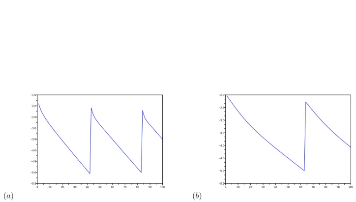
3.4.3 Some numerical results
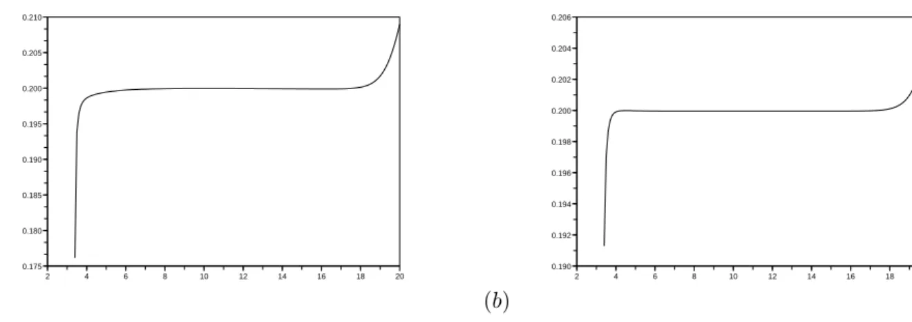
We show here some numerical results derived from the Finite Element Methods applied to European and American options in dimension 1. Two types of finite elements were used: “hat” functions and cubic splines. We see on Figures (3.1)–(3.2) that the Finite Element Method based on the cubic splines (with the same size of the mesh) computes price much better (in the sense of the implicit volatilities) than “hat functions” does.
We present just below numerical results about the convergence of the projected gradient method for the American options using the same finite elements as in the European case just above. In Fig. 3.3, we can the error of the “inner” iterate Un (see question 7 in
Subsection 3.4.2) as respect to n. At each time step, we can see that the line is broken. It means that the gradient is restarted with the new updated second member. We can see also that more iteration is needed in the cubic spline case than in the “hat” functions case. Indeed more precision gives more information about the free frontier at each time step. It is why we need more iteration.
(a) 2 4 6 8 10 12 14 16 18 20 0.175 0.180 0.185 0.190 0.195 0.200 0.205 0.210 (b) 2 4 6 8 10 12 14 16 18 20 0.190 0.192 0.194 0.196 0.198 0.200 0.202 0.204 0.206
Figure 3.1: Implicit Volatility as a function of the spot in the case: (a) “hat” functions; (b) cubic splines. European put option r = 0.1, σ = 0.2, K = 10, T = 1. In both case M = 200 elements on (0, 20). (a) 2 4 6 8 10 12 14 16 18 0.398 0.399 0.400 0.401 0.402 0.403 0.404 0.405 0.406 0.407 0.408 (b) 2 4 6 8 10 12 14 16 18 0.3999 0.4000 0.4001 0.4002 0.4003 0.4004 0.4005
Figure 3.2: Implicit Volatility as a function of the spot in the case: (a) “hat” functions; (b) cubic splines. European put option r = 0.1, σ = 0.4, K = 10, T = 1. In both case M = 200 elements on (0, 20).
(a) 0 10 20 30 40 50 60 70 80 90 100 −5.5 −5.0 −4.5 −4.0 −3.5 −3.0 −2.5 −2.0 −1.5 (b) 0 10 20 30 40 50 60 70 80 90 100 −5.5 −5.0 −4.5 −4.0 −3.5 −3.0 −2.5 −2.0
Figure 3.3: Error kUn+1 − Unk2 with respect to n: iteration of the projected gradient
Asian options
We end these notes by an example of path-dependant exotic options: the Asian options and try to give some clues about its numerical implementation. This problem is derived from [2]. See also [6] for the original derivation of the equation.
Let K and T be two positive real. We are interested by the pricing of an Asian op-tion with fixed strike K and maturity T (European contract). Hence, the payoff funcop-tion depends now on the whole trajectory of the risky asset S = (St) (6= Vanilla options):
Vt= E µ e−r(T −t) µ 1 T Z T 0 Stdt − K ¶ + | Ft ¶ , (4.0.1)
where Ftdenotes the filtration of B = (Bt).
We set for any t ≥, ¯St = 1tR0tSsds. The same techniques which has allowed us to
derive the Black & Scholes PDE in the first Chapter show here that Vt= v(t, St, ¯St) where
v = v(t, x, y) satisfies the PDE: ∂ v ∂t + rx ∂ v ∂x + σ2x2 2 ∂2v ∂x2 + µ x − y t ¶ ∂v ∂y − rv = 0, (x, y) ∈ R ∗ +, t ∈ [0, T [, (4.0.2)
with the terminal condition:
v(T, x, y) = (y − K)+, x > 0, y > 0.
(4.0.3)
1. We set for any t ∈ [0, T ] and x, y > 0,
z = K − yt/T
x , and f (t, z) = 1
xv(t, x, y). Show that f is the solution of the following PDE:
∂ f ∂t + σ2z2 2 ∂2f ∂z2 − µ 1 T + rz ¶ ∂f ∂z = 0, z ∈ R, (4.0.4)
with the terminal condition:
f (T, z) = z−= max(0, −z).
(4.0.5)
Figure 4.1: Domaine de calcul
3. (a) We set now g(t, x) = f (t, x − t/T ). Show that g satisfies the following PDE: ∂g ∂t + σ2 2 µ x − t T ¶2 ∂2g ∂x2 − r µ x − t T ¶ ∂g ∂x = 0, x ∈ R, t ∈ [0, T [, (4.0.6)
with the terminal condition:
g(T, x) = (1 − x)+.
(4.0.7)
3. (b) Let ef the solution of (4.0.4) obtained with the terminal data ef (T, z) = −z. Show that e f (t, z) = 1 rT ³ 1 − e−r(T −t)´− z e−r(T −t). Deduce from this that for any x ≤ t/T , we have
g(t, x) = 1 rT ³ 1 − e−r(T −t)´− µ x − t T ¶ e−r(T −t). (4.0.8)
4. We remark that (4.0.6) is equivalent to
∂g ∂t + σ2 2 ∂ ∂x õ x − t T ¶2 ∂ g ∂x ! − (r + σ2) µ x − t T ¶ ∂g ∂x = 0, x ∈ R, t ∈ [0, T [, (4.0.9)
Let N ≥ 1 an integer and ∆t = 1/N . We discretize (4.0.9) by means of a Crank– Nicolson scheme with uniform time step ∆t. As regard the space, we want to exploit the fact that we know the solution at the left of the line x = t/T (cf (4.0.9). Therefore, we discretize (0, L) as shown in Figure 4.1 and we set ∆x = 1/N in order to numerically capture the line x = t/T . We complete between 1 and L by adding J intervals in order to have L = (N + J)∆x.
We set xi = i∆x for 1 ≤ i ≤ N + J et xi±1/2 = (i ± 1/2)∆x.
What are the order of approximation of the following finite differences ? (a) 1 ∆x ½¡ xi+1/2− t/T¢2 g(t, xi+1) − g(t, xi) ∆x − ¡ xi−1/2− t/T¢2 g(t, xi) − g(t, xi−1) ∆x ¾ for ∂ ∂x µ (x − t/T )2 ∂g ∂x ¶ (t, xi) and (b)
1 2 ½¡ xi+1/2− t/T¢ g(t, xi+1) − g(t, xi) ∆x + ¡ xi−1/2− t/T¢ g(t, xi) − g(t, xi−1) ∆x ¾ for (x − t/T )∂ g ∂x(t, xi) ?
5. We choose Dircihlet boundary conditions on the frontier x = t/T and Neumann type boundary conditions on x = L compatible with the terminal data. Give a second order approximation of the Neumann boundary condition on x = L for (4.0.7)–(4.0.9).
6. Derive the following matrix formulation
(I + ∆tBk)Gk+1 = (I − ∆t fBk)Gk, 0 ≤ k ≤ N,
where Gk is the vector whose composants are g(t k, xi).
Appendix A : Some useful Scilab
scripts (volimp.sci file)
function [y]=myerf(x) y=0.5*(1+erf(x/sqrt(2))); endfunction
//////////////////////////////////////// // Put BS closed form : scalar version ////////////////////////////////////////
function [p,p_sig]=BSPut_s(x,K,r,sig,theta) // scalar definition if (theta<=%eps) then p=max(K-x,0); p_sig=0; else d1=(log(x/K)+(r+sig^2/2)*theta)/(sig*sqrt(theta)); d2=d1-sig*sqrt(theta);
p=K*exp(-r*theta)*myerf(-d2) - x(~(x==0)).*myerf(-d1) // Prix Put p_sig=x*exp(-d1^2/2)*((r+sig^2/2)*theta-log(x/K)) ... // Drive Put/Vol
- K*exp(-r*theta-d2^2/2)*((r-sig^2/2)*theta-log(x/K)) p_sig=p_sig/(sqrt(2*%pi*theta)*sig^2)
end
///////////////////////////////////////////// // Put BS closed form : vectorized version /////////////////////////////////////////////
function [p,p_sig]=BSPut_v(x,K,r,sig,theta) // vectorized def // x Vecteur des spots
// sigma vecteur des vol
// p en sortie : vecteur des prix de Puts sig=abs(sig); p=zeros(x); p_sig=zeros(x); un=ones(x); zer=zeros(x); if (theta<=%eps) then 45
p = max( K - x, 0) else
p(x==0) = K*exp(-r*theta)*un(x==0); // Cas x==0 p_sig(x==0) = zer(x==0);
p(sig==0) = max(K*exp(-r*theta) - x(sig==0),0); // Cas sig=0 p_sig(sig==0) = zer(sig==0); reste=~(x==0 | sig==0); signo=sig(reste); xno=x(reste); d1=(log(xno/K)+(r+signo.^2/2)*theta)./(signo*sqrt(theta)); d2=d1-signo*sqrt(theta);
p(reste)=K*exp(-r*theta)*myerf(-d2) - xno.*myerf(-d1) // Put Price p_sig(reste)=xno.*exp(-d1^2/2).*((r+signo.^2/2)*theta-log(xno/K)) ... // Put Delta
- K*exp(-r*theta-d2^2/2).*((r-signo.^2/2)*theta-log(xno/K)) p_sig(reste)=p_sig(reste)./(sqrt(2*%pi*theta)*signo.^2)
end
endfunction
////////////////////////////////////////// // Implicit volatility from Put prices //////////////////////////////////////////
function [s,y,ind,iternwt,err]=volimpP_v(x,K,r,sig0,theta,Put,tol) // x vecteur des spots
// sig0 vecteur des vol initiales du Newton // Put vecteur des prix de Put
// Mme taille pour les trois ( + tous vecteurs lignes) ! sig=abs(sig0); sig1=zeros(sig0); err=ones(x); imxnwt=100; stop=(norm(err)<=tol); iternwt=1; while (iternwt<=imxnwt)&(~stop) [p,p_sig]=BSPut_v(x,K,r,sig,theta); tronc=(abs(p_sig)<=tol); err(~tronc)=abs(p(~tronc)-Put(~tronc));
sig(~tronc) = sig(~tronc) - (p(~tronc) - Put(~tronc))./p_sig(~tronc); stop=(norm(err(~tronc))<=tol) iternwt=iternwt + 1; end s=sig(~tronc) y=x(~tronc) ind=~tronc endfunction
Appendix B : Scilab scripts for
Finite Difference methods for
pricing
B.1. European and American, dimension 1
//////////////////////////////////////////////////// // CIMPA HANOI 23/04/2007 - 4/05/2007
// Finite Difference Method for American options //////////////////////////////////////////////////// clear; ///////////////////////////// // MODEL PARAMETER (BS) ///////////////////////////// r=0.1; sigma=0.2; //////////////////////////////////////// // OPTION PARAMETER //////////////////////////////////////// // Cf. Option Pricing, Wilmott et al, p. 335 T=1; K=10; deff(’[payoff]=h(x)’,[’payoff=max(K-x,0)’]); // Spatial discretization M=200; L=2*K; Deltax=L/(M+1); // Time discretization N=100; Deltat=T/N; theta=0.5; imxtmp=N;
// Centrage, dcentrage des drives d’ordre 1 en x centrex=%T;
// Conditions aux bords
D = spzeros(M+2,M+2); // Dirichlet N = spzeros(M+2,M+2); // Neumann
D(1,1) = 1.0; // Dirichlet Boundary Conditions at x=0 N(M+2,M+2) = 1.5; // Neumann 2nd order at x=L N(M+2,M+1) = -2.0; N(M+2,M) = 0.5; //N(M+2,M+2) = 1.0; // Neumann 1st order //N(M+2,M+1) = -1.0; //D(M+2,M+2) = 1.0; // D. B. C. at x=L //////////////////////////// // DO NOT EDIT BELOW
//////////////////////////// // Elementary matrices x=linspace(0,L,M+2); xint=x(2:M+1);
// Sparse definition of the elementary matrices Lx = spzeros(M+2,M+2); Gd = spzeros(M+2,M+2); Gc = spzeros(M+2,M+2); auxLx = -2.0/Deltax^2*speye(M+2,M+2) + ... 1.0/Deltax^2*diag(sparse(ones(M+1,1)),1) + ... 1.0/Deltax^2*diag(sparse(ones(M+1,1)),-1); auxGd = 1.0/Deltax*diag(sparse(ones(M+1,1)),1) - ... 1.0/Deltax*speye(M+2,M+2); auxGc = 0.5/Deltax*diag(sparse(ones(M+1,1)),1) - ... 0.5/Deltax*diag(sparse(ones(M+1,1)),-1); Lx = [ zeros(1,M+2) ; auxLx(2:M+1,:) ; zeros(1,M+2)]; Gd = [ zeros(1,M+2) ; auxGd(2:M+1,:) ; zeros(1,M+2)]; Gc = [ zeros(1,M+2) ; auxGc(2:M+1,:) ; zeros(1,M+2)]; Bext = D + N;
Idint = speye(M+2,M+2) - spones(diag(spones(diag(Bext)))); Bint = 0.5*sigma^2*diag(sparse(x.*x))*Lx - r*Idint; if centrex==%F then
Bint = Bint + r*diag(sparse(x))*Gd; else
Bint = Bint + r*diag(sparse(x))*Gc; end;
// Matrix to be inversed
A = Idint - theta*Deltat*Bint + Bext; [hh,rk]=lufact(A);
[P,L,UU,Q]=luget(hh); // Donne initiale
U0=h(x)’; // Cash-or-Nothing Call //U0=1*(x>K)’; ///////////////////// // Time iterates ///////////////////// itertmp=1;
U=U0; // European price V=U0; // american price while itertmp<=imxtmp
// Second member updated at each time iteration (European case) Fint = Idint*U + (1 - theta)*Deltat*Bint*U;
Fext = zeros(M+2,1);
Fext(1) = K*exp(-r*Deltat*itertmp); // European price
U=lusolve(hh,Fint + Fext);
// Second member updated at each time iteration (American case) Fint_am = Idint*V + (1 - theta)*Deltat*Bint*V;
Fext_am = zeros(M+2,1); Fext_am(1) = U0(1); Fext_am(M+2) = U0(M+2);
// Projected LU : American price V = P’*(Fint_am + Fext_am); PU0 = P’*U0;
V = L\V; for i=M+2:-1:1,
V(i) = max(PU0(i),V(i) - sum(UU(i,i+1:M+2)’.*V(i+1:M+2))); end V = Q’*V; xbasc(); //plot2d(xx,v,leg="Iter="+string(itertmp*Dt),rect=[a,ymin,b,ymax]) plot2d(x,[V,U,U0],leg="Iter="+string(itertmp*Deltat)) itertmp = itertmp + 1; end
A.2. European dimension 2
//////////////////////////////////////////////////////// // CIMPA HANOI 23/04/2007 - 4/05/2007
// Finite Difference Method for 2D European options //
// Ex : Put on the minimum of two assets
//////////////////////////////////////////////////////// clear
L1=20; L2=20; M1=50; M2=50; centrex=%T; centrey=%T; /////////////////////////////////////////// // Loading of the elementary DF matrices /////////////////////////////////////////// load(’BS2d_assemb_DF_centrex’ + string(centrex) + ... ’_centrey’ + string(centrey) + ... ’_L1-’ + string(L1) + ... ’_L2-’ + string(L2) + ... ’_Mx’+string(M1) + ... ’_My’+string(M2) + ’.save’); ///////////////////////// // BS MODEL PARAMETER ///////////////////////// s1 = 0.2; s2 = 0.2; mu1 = 0.; mu2 = 0.; rho = 0.5; r = 0.1; /////////////////////////// // OPTION PARAMETER /////////////////////////// T=1; K=10; deff(’[payoff]=h(x,y)’,[’payoff=max(K - min(x,y),0)’]); //////////////////////////// // MATRICES //////////////////////////// wLx=matrix(x’*ones(1,M2+2), (M1+2)*(M2+2),1)^2*s1^2/2; wMxy=matrix(x’*y, (M1+2)*(M2+2),1)*rho*s1*s2; wLy=matrix(ones(M1+2,1)*y, (M1+2)*(M2+2),1)^2*s2^2/2; wGx=r*matrix(x’*ones(1,M2+2),(M1+2)*(M2+2),1); wGy=r*matrix(ones(M1+2,1)*y, (M1+2)*(M2+2),1); // BOUNDARY CONDITIONS D = spzeros((M1+2)*(M2+2),(M1+2)*(M2+2)); // Dirichlet N = spzeros((M1+2)*(M2+2),(M1+2)*(M2+2)); // Neumann Fext=zeros((M1+2)*(M2+2),1); i=M1+2; for j=2:M2+1 // x = L1 k=i+(j-1)*(M1+2); N(k,k) = 1.5;
N(k,k-1) = -2.0; N(k,k-2) = 0.5; end i=1; // x = 0 for j=1:M2+2 k=i+(j-1)*(M1+2); D(k,k) = 1.0; end j=M2+2; // y = L2 for i=2:M1+1 k=i+(j-1)*(M1+2); N(k,k) = 1.5; N(k,k-M1-2) = -2.0; N(k,k-2*M1-4) = 0.5; end j=1; // y = 0 for i=2:M1+2 k=i+(j-1)*(M1+2); D(k,k) = 1.0; end Bext = D + N;
// MATRICES OF THE BS OPERATOR
Idint=speye((M1+2)*(M2+2),(M1+2)*(M2+2)) - spones(diag(spones(diag(Bext)))); Bint=diag(sparse(wLx))*Lx + diag(sparse(wLy))*Ly ... + diag(sparse(wMxy))*Mxy + diag(sparse(wGx))*Gx ... + diag(sparse(wGy))*Gy ... - r*Idint; /////////////////////////// // TIME ITERATIONS /////////////////////////// N=100 Deltat=T/N; theta=0.5; imxtmp=100; // Matrix to be inversed
A = Idint - theta*Deltat*Bint + Bext; [hh,rk]=lufact(A);
// Initial data
U0=matrix(h(x’*ones(1,M2+2),ones(M1+2,1)*y),(M1+2)*(M2+2),1); itertmp=1;
while itertmp<=imxtmp
Fint=Idint*U + (1-theta)*Deltat*Bint*U;
Fext(1+(0:M2+1)*(M1+2)) = K*exp(-r*Deltat*itertmp); // Non homogeneous Dirichlet at x=0 Fext(1:M1+2) = K*exp(-r*Deltat*itertmp); // Non homogeneous Dirichlet at y=O U=lusolve(hh,Fint+Fext);
itertmp=itertmp+1; end
// Plotting of the solution m=228; n= fix(3/8*m); rr=[(1:n)’/n; ones(m-n,1)]; g=[zeros(n,1); (1:n)’/n; ones(m-2*n,1)]; b=[zeros(2*n,1); (1:m-2*n)’/(m-2*n)]; hhh=[rr g b]; xset("colormap",hhh) v=matrix(U,M1+2,M2+2); xbasc(); plot3d1(x,y,v);