HAL Id: ensl-00476007
https://hal-ens-lyon.archives-ouvertes.fr/ensl-00476007
Submitted on 23 Apr 2010
HAL is a multi-disciplinary open access
archive for the deposit and dissemination of
sci-entific research documents, whether they are
pub-lished or not. The documents may come from
teaching and research institutions in France or
abroad, or from public or private research centers.
L’archive ouverte pluridisciplinaire HAL, est
destinée au dépôt et à la diffusion de documents
scientifiques de niveau recherche, publiés ou non,
émanant des établissements d’enseignement et de
recherche français ou étrangers, des laboratoires
publics ou privés.
Time-Varying Spectrum Estimation of Uniformly
Modulated Processes by Means of Surrogate Data and
Empirical Mode Decomposition
Azadeh Moghtaderi, Patrick Flandrin, Pierre Borgnat
To cite this version:
Azadeh Moghtaderi, Patrick Flandrin, Pierre Borgnat. Time-Varying Spectrum Estimation of
Uni-formly Modulated Processes by Means of Surrogate Data and Empirical Mode Decomposition. IEEE
International Conference on Acoustics, Speech, and Signal Processing ICASSP-10, Mar 2010, Dallas,
Texas, United States. �ensl-00476007�
TIME-VARYING SPECTRUM ESTIMATION OF UNIFORMLY MODULATED PROCESSES
BY MEANS OF SURROGATE DATA AND EMPIRICAL MODE DECOMPOSITION
Azadeh Moghtaderi, Patrick Flandrin and Pierre Borgnat
´
Ecole Normale Sup´erieure de Lyon, Laboratoire de Physique
46 all´ee d’Italie 69364 Lyon Cedex 07, France
ABSTRACT
We propose a new estimate of the time-varying spectra of uni-formly modulated processes. The estimate is based on a re-sampling scheme which incorporates empirical mode decom-positions and surrogate data techniques. The performance of the method is studied via simulations.
Index Terms— Bandlimited signals, spectral analysis,
stochastic processes, time-frequency analysis
1. INTRODUCTION
Estimation of the time-varying spectra (TVS) of nonstation-ary processes remains a challenging problem. This is because (i)many different types of nonstationarity exist and(ii)in con-trast with the stationary ergodic case, time averaging cannot be used as a substitute for ensemble averaging to reduce fluc-tuations in estimates. Although no “universal solution” is ex-pected to exist for all types of nonstationarity, specific ap-proaches can be developed for restricted classes.
In this paper, we focus on the class of uniformly modu-lated processes (UMPs). Theoretically, UMPs have a simple mathematical form, since they can be decomposed into a sta-tionary process multiplied by a modulating function. More pragmatically, UMPs have been used successfully as mod-els of various real-world processes, e.g., in seismology (see [1], [2] and [3]). We propose here a method for estimating the TVS of a UMPXXX. The method combines an estimate of
the TVS obtained by BCMOTIFS estimator introduced in [4] with surrogate data techniques, and proceeds in three steps. The first step estimates the modulating function ofXXX via an
empirical mode decomposition. The second step determines the “stationary component” ofXXX; surrogate data techniques
are then used to create additional “virtual” realizations ofXXX.
These realizations are then used to compute a more accurate estimate of the TVS ofXXX which is based on the arithmetic
averaging of BCMOTIFS estimates for each realization. In Section 2, we briefly review the UMPs, empirical mode decompositions, and surrogate data techniques. In Sections 3 and 4, we describe in detail the estimation method sketched in the previous paragraph. Finally, in Section 5, we examine the performance of the method on simulated data.
2. PRELIMINARIES 2.1. Uniformly modulated processes
LetXXX = {Xt}t∈Zbe a discrete-time,R-valued, zero-mean,
finite-variance nonstationary process. We say that XXX is a
uniformly modulated process (UMP) if there exists a
zero-mean stationary processYYY = {Yt}t∈Z with spectrum SYYY
and a sequence{Ct}t∈Z of positive real numbers, such that
Xt= CtYtfor eacht ∈ Z. We refer to Ctas the modulating function ofXXX, and YYY is the stationary component of XXX. We
assume that the modulating function is “slowly–varying” in comparison withYYY . More precisely, the modulating function
is a bandlimited baseband process whileYYY is a broadband
process without any low-frequency oscillations.
The time-varying spectrum (TVS) [5] of a UMPXXX is
de-fined byTXXX(t, f ), Ct2SYYY(f ) for (t, f ) ∈ Z × [−1/2, 1/2].
2.2. Surrogate data techniques
Surrogate data techniques comprise a type of resampling
technique. Given a single realization of a stochastic process
Y
YY , surrogate data techniques can produce an arbitrary number
of “virtual” realizations ofYYY , called surrogates, with similar
statistical properties. Originally, surrogates were used to test for nonlinearity [6]; more recently, they were used in [7, 8] to test for nonstationarity. In the latter, the rationale is that, given the same global empirical spectrum, a nonstationary process differs from a stationary one by some structure in time which carries over to the “phase” of the spectrum. Randomizing the phase and keeping the magnitude unchanged leads therefore to a “stationarized” process, while many other realizations can be obtained due to randomization of the phase. In a non-stationary context, this allows the construction of a statistical reference corresponding to the null hypothesis of stationarity. However if the process under study is stationary—as it will be assumed in the following—surrogates can be viewed as virtual realizations.
2.3. Empirical mode decompositions
LetStbe an arbitrary signal. Briefly, the empirical mode de-composition (EMD) [9] is a model-free and fully data-driven
oscillations into its zero-mean oscillatory components. This is achieved by a “fine-to-coarse” recursive scheme: The fastest local oscillations (identified through neighbouring local ex-trema) are subtracted from the signal, yielding a residual sig-nal to which the same procedure can be applied. Extracted in this way, each of the components is referred to as an
intrin-sic mode function (IMF) ofSt. The recursion stops when the
residual signal has no more oscillation. Denoting IMFs by
Mt(i)for1 ≤ i ≤ Imax, we write
St= IXmax
i=1
Mt(i)+ ρt, (1)
whereρtis the residual signal. For MATLAB code and
fur-ther details concerning implementation of the EMD, see [10].
3. TIME-VARYING SPECTRUM ESTIMATION BY MEANS OF SURROGATE DATA
LetXXX be a UMP with modulating function Ctand stationary
componentYYY . In this section, we describe a general technique
to estimateTXXX, based on the use of surrogate data.
Let X = X0, X1, . . . , XN−1be a realization ofXXX, and
let bCtbe a nonzero estimate ofCtfor eacht. Set ˜Yt= Xt/ bCt
for eacht. Provided that each bCtestimatesCtaccurately (see
Section 4 for details), ˜Y = ˜Y0, ˜Y1, . . . , ˜YN−1can be regarded as a realization ofYYY . We use ˜Y to obtainJ surrogate data sets
˜ Yj= ˜Yj 0, ˜Y j 1, . . . , ˜Y j N−1, where1 ≤ j ≤ J. Define X˜j = Cb 0Y˜0j, bC1Y˜1j, . . . , bCN−1Y˜N−1j , where
again1 ≤ j ≤ J. We call ˜Xjthejth nonstationary surro-gate data obtained from X and regard this data as elements
of the ensemble ofXXX. For each 1 ≤ j ≤ J, let bTXXXj be an
estimate ofTXXXbased solely onX˜j. We take the arithmetic
average of the bTXXXj as an estimate of TXXX, which we call the averaged surrogate-based estimate:
b Tav X X X(t, f ), 1 J J X j=1 b TXXXj(t, f ), (t, f ) ∈ Z × [−1/2, 1/2].
In this paper, we choose each bTXXXj to be the BCMOTIFS esti-mator [4, 11]. The rationale behind this choice is as follows: For general processes, theoretical and simulation results in [4] indicate BCMOTIFS has lower bias and variance than other estimators of the TVS, especially near the boundaries of the time-frequency region. In particular, for UMPs, BCMOTIFS is approximately unbiased [4].
4. MODULATING FUNCTION ESTIMATION
LetXXX and X be as in Section 3, and assume that Xt6= 0 for
eacht. To proceed with the technique proposed in Section 3,
we must estimate eachCt. In this section, we describe how
Ctand X can be “decoupled,” leading to an estimate ofCt.
DefineX∗
t = log |Xt|, so that Xt∗= log Ct+ log |Yt| for
eacht. Write X∗= log |X
0|, log |X1|, . . . , log |XN−1|. We
can compute the EMD of X∗ to obtain its IMFsMt(i), and
writeX∗
t as in Eq. (1) whenStis replaced byXt∗. Note that
the applicability of EMD method in general, does not require particular forms of oscillations and therefore appropriate for the log-transformed signal. Loosely speaking, the assumption made in Section 2.1 states that the oscillations oflog Ctare
much slower than those inlog |Yt|. As a result the oscillations
oflog Ctare accurately described by a set of high-order IMFs
such that for1 ≤ i∗≤ Imaxwe have
log Ct≈ IXmax
i=i∗
Mt(i)+ ρt. (2)
Following above, estimatingCtreduces to determiningi∗.
We now describe three approaches to determiningi∗.
The energy of theith IMF is defined by E(i)=PN−1 t=0 |M
(i) t |2
for eachi. For typical broadband signals, E(i)is decreasing
in i [12]. Identifying the smallest index i + 1 such that E(i+1) > E(i) can therefore provide information about the
value ofi∗. This is called the energy approach.
Denote the number of zero crossings of the ith IMF by Z(i). It can be observed that, in the absence of low-frequency
oscillations, broadband signals give rise to a family of IMFs satisfyingR(i+1) ≈ 2, where R(i+1) = Z(i)/Z(i+1)
when-ever it is defined. Furthermore, we assume that the random variablesR(i+1) are approximately equally distributed. We
callR(i+1)theith ratio of zero crossing numbers (ith RZCN).
Hence the smallest indexi + 1 for which R(i+1)is
“signifi-cantly different” from 2 can provide information about the value ofi∗. The question is how to quantify “significantly
different.” To answer this question, we construct 13 processes (all approximately broadband without low-frequency oscilla-tions), including(i)nine fractional Gaussian noise processes with Hurst exponentsH = 0.1, 0.2, . . . , 0.9,(ii)two AR(2) processes, and(iii)two nonstationary processes, the first being AR(2) with time-dependent coefficients and the second being frequency-modulated. For each process, we create 5000 re-alizations of lengthN = 1000, and compute the EMDs and
RZCN of each. We then compute the empirical distribution of
~
R = [ ~R1R~2 · · · ~R5000] where denoting the ith RZCN of the
bth realization by R(i+1)b ,1 ≤ i ≤ Ib max− 1, we have ~Rb = [R(2)b R (3) b · · · R (Ib max)
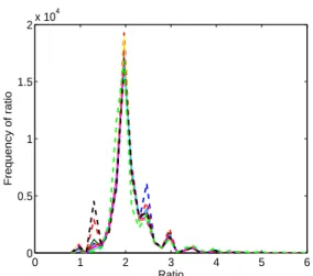
b ] for 1 ≤ b ≤ 5000. Fig. 1 shows the
empirical distribution of ~R computed for each process and
shown in different colors. The result of our simulations en-courages the idea that, regardless of the type of broadband process, the distribution of ~R remains unchanged. As a result
of this, we may then propose a common threshold test for de-termining whenR(i+1)is significantly different from2. For
each process, we compute the empirical distribution ofR(i+1)
over all the realizations and for eachi = 1, 2 . . . , Imax− 1
re-spectively where here we assumeImax= 10. In this case, if,
as an example, for a particular realization, we haveImax= 8,
we assumeR(8) = R(9) = R(10)and ifI
max = 12, we
0 1 2 3 4 5 6 0 0.5 1 1.5 2x 10 4 Ratio Frequency of ratio
Fig. 1. Empirical distribution of ~R computed for different
processes (different colors). Apart from the expected peak at 2, there exist several smaller but visible peaks. They appear in the presence of high order IMFs which have small values of zero crossing numbers.
2 4 6 8 10 1.5 2 2.5 3 3.5 Ratio index
Right and left threshold
Fig. 2. The right and left thresholds (marked by stars)
com-puted for different processes (different colors). Solid lines indicate averaged left and right thresholds and dashed lines indicate two standard deviation of the averaged thresholds. of each distribution, and refer to them asith right and left
thresholds respectively. Fig. 2 shows the right and left
thresh-olds for each process (different colors). Any RZCN which is outside of the two standard deviation of the averagedith left
and right thresholds within 13 process is significantly
differ-ent from 2. Finally, as mdiffer-entioned earlier, the smallest index
i+1 where R(i+1)is significantly different from 2 determines
i∗. The problem is that since the selection of the left and right
thresholds are entirely based on an empirical result, it is al-ways possible that the smallesti + 1 is a false detection and
not the correcti∗. This approach is called the ratio approach.
The energy and ratio approaches can be combined in order to reduce the number of false detects as follows: For each
1 ≤ i ≤ Imax− 1, we compute each index i + 1 such that
E(i+1) > E(i). We also evaluate every indexi + 1 where
R(i+1)is significantly different from 2. We then choosei ∗to
be the smallest common index in both approaches. The value ofi∗is then plugged into Eq. (2) in order to evaluatelog Ct.
The estimated modulating function is bCt= exp(log Ct). This
combined approach is called the energy-ratio approach.
5. NUMERICAL EXAMPLES
LetXXX(k) = {X(k)
t }t∈Z,1 ≤ k ≤ 5 be UMPs with
modulat-ing functions Ct(1)= e −(t−500)22(200)2 , Ct(2)= p 1 + t/T Ct(3)= 2 + sin(2πpt), C (4) t = 1.5 + cos(2πqt) Ct(5)= 2 − e −(t−500)22(200)2 ,
whereT = 200, p = 0.002 and q = 0.001. The stationary
components of theXXX(k)are as follows:YYY(1),YYY(2), andYYY(3)
are fractional Gaussian noise with Hurst parametersH = 0.2, H = 0.5, and H = 0.8, respectively, and YYY(4)andYYY(5)are
the AR(2) processes
Yt(4) = 0.2Y (4) t−1+ 0.5Y (4) t−2+ ζt Yt(5) = 0.8Y (5) t−1− 0.4Y (5) t−2+ ǫt.
Here,{ζt}t∈Zand{ǫt}t∈Zare independent white noise
pro-cesses with variance104.
For each k, we create 5000 realizations of length N = 1000 of XXX(k) and compute the EMD for each realization. We then apply the energy, ratio, and energy–ratio approaches to each realization and each UMP to evaluate i∗, denoted
i∗,a(k), where a = 1, 2, 3 indicate energy, ratio and energy–
ratio approaches respectively. Using our theoretical knowl-edge of the modulating function for each UMP, we picki∗
which gives the minimumL2-distance betweenlog C tfrom
Eq. (2) and theoretical log modulating function. We de-notei∗ obtained from minimumL2-distance by i†(k).
Ta-ble 1 shows the number of times in 5000 where we have obtained i∗,a(k) = i†(k), i∗,a(k) = i†(k) + 1, i∗,a(k) =
i†(k) − 1, or |i∗,a(k) − i†(k)| > 1. It is clear from Table
1 that the energy–ratio approach outperforms the other two approaches. We now takeXXX(4) for further analysis. Let
X = X0, X1, . . . , XN−1 be a realization ofXXX(4) and X∗
the log-transform of X . We compute the EMD of X∗ to obtain its IMFs and then evaluateE(i)andR(i+1)for eachi.
Fig. 3 shows the plot ofE(i),1 ≤ i ≤ I
max, (top plot) and
R(i+1),1 ≤ i ≤ I
max− 1, (bottom plot) where Imax = 9
in this example. Applying the energy approach we determine that there are 4 indexesi + 1 where i = 3, 5, 7, 8 which
sat-isfiesE(i+1) > E(i). On the other hand, applying the
ra-tio approach, we find out that there are three indexesi + 1
fori = 6, 7, 8 where R(i+1)is significantly different from 2.
These indexes are marked by red triangles in Fig 3. Applying the energy–ratio approach, we see that the first common index between the two approaches isi∗= 8.
Usingi∗ = 8, we evaluate bCt(see Section 4). The
Energy Ratio Energy–Ratio a= 1 a= 2 a= 3 i∗,a(1) = i†(1) 2361 1926 3193 i∗,a(1) = i†(1) + 1 1353 918 717 i∗,a(1) = i†(1) − 1 583 484 891 |i∗,a(1) − i†(1)| > 1 703 1672 199 i∗,a(2) = i†(2) 1866 1420 2697 i∗,a(2) = i†(2) + 1 1181 735 948 i∗,a(2) = i†(2) − 1 658 495 949 |i∗,a(2) − i†(2)| > 1 1295 2350 406 i∗,a(3) = i†(3) 1919 1339 2710 i∗,a(3) = i†(3) + 1 1386 902 985 i∗,a(3) = i†(3) − 1 373 521 910 |i∗,a(3) − i†(1)| > 1 1322 2238 395 i∗,a(4) = i†(4) 2636 1893 3316 i∗,a(4) = i†(4) + 1 1100 980 643 i∗,a(4) = i†(4) − 1 232 492 740 |i∗,a(4) − i†(4)| > 1 1032 1635 301 i∗,a(5) = i†(5) 2615 1487 3598 i∗,a(5) = i†(5) + 1 1056 902 637 i∗,a(5) = i†(5) − 1 295 363 529 |i∗,a(5) − i†(5)| > 1 1034 2248 236
Table 1. Comparison between energy, ratio and energy–ratio
approaches using the theoreticallog Ctfor 5 UMPs.
1 2 3 4 5 6 7 8 9 5 10 15 Energy of IMFs Index of IMFs 1 2 3 4 5 6 7 8 9 0 2 4 6 Index of RZCN RZCN
Fig. 3.E(i),i = 1, 2, . . . , 9 (top) and R(i+1),i = 1, 2, . . . , 8
(bottom). The red triangles mark the indexes which satisfy the conditions in energy (top) and ratio (bottom) approaches. dataX˜j,1 ≤ j ≤ 50 (see Section 3). Using 50
nonstation-ary surrogate data, we then estimateTXXX using the averaged
surrogate-based estimate bTav X X
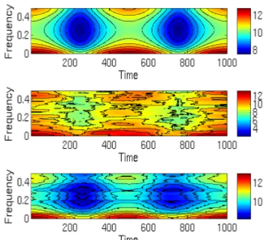
X (see Section 3). Fig. 4 shows
the performance of this estimator in comparison with the BC-MOTIFS estimator for X .
6. CONCLUSION
In this paper, we proposed a new scheme to estimate the time-varying spectra of uniformly modulated processes. The esti-mate proceeds by computing “virtual” realizations, using sur-rogate data and empirical mode decompositions. Simulation results suggest that the new estimator performs well, and af-fords a significant improvement over BCMOTIFS.
Fig. 4. Theoretical TVS ofXXX(4) (top), estimate of the TVS
using X (middle), estimate of the TVS usingX˜j,1 ≤ 1 ≤
50 (bottom). The parameters used in BCMOTIFS estimator
areN W = 4, K = 7 and B = 201.
7. REFERENCES
[1] L. J. Herbst, “Periodogram analysis and variance fluctuation,” Journal
of the Royal Statistical Society, Series B, vol. 25, pp. 442–450, 1963.
[2] T. Fujita and H. Shibara, “On a model of earthquake ground motions for response analysis and some examples of analysis through experiment,”
Conference on Engineering Design for Earthquake Environments, vol.
12, pp. 139–148, 1978.
[3] G. R. Dargahi-Noubary and P. J. Laycock, “Special ratio discriminant and information theory,” Journal of Time Series Analysis, vol. 2, no. 2, pp. 71–85, 1981.
[4] A. Moghtaderi, Multitaper Methods for Time-Frequency Spectrum Estimation and Unaliasing of Harmonic Frequencies, Ph.D. thesis,
Queen’s University, 2009.
[5] G. M´elard and A. H. Schutter, “Contributions to evolutionary spectral theory,” Journal of Time Series Analysis, vol. 10, no. 1, pp. 41–63, 1989.
[6] J. Theiler, S. Eubank, A. Longtin, B. Galdrikian, and J. D. Farmer, “Testing for nonlinearity in time series: the method of surrogate data,”
Physica D, vol. 58, no. 1–4, pp. 77–94, 1992.
[7] J. Xiao, P. Borgnat, and P. Flandrin, “Testing stationarity with time-frequency surrogates,” in Proceedings of EUSIPCO-07, Pozna´n, Poland, 2007, pp. 2020–2024.
[8] J. Xiao, P. Borgnat, P. Flandrin, and C. Richard, “Testing stationarity with surrogates—a one-class SVM approach,” in Proceedings of the
IEEE Statistical Signal Processing Workshop (SSP-07), Madison, WI,
2007, pp. 720–724.
[9] N. E. Huang, Z. Shen, S. R. Long, M. L. Wu, H. H. Shih, Q. Zheng, N. C. Yen, C. C. Tung, and H. H. Liu, “The empirical mode decompo-sition and Hilbert spectrum for nonlinear and non-stationary time series analysis,” Proceedings of the Royal Society of London A:
Mathemati-cal, Physical and Engineering Sciences, vol. 454, pp. 903–995, 1998.
[10] G. Rilling, P. Flandrin, and P. Gonc¸alves, “On empirical mode decom-position and its algorithms,” in IEEE-EURASIP Workshop on
Nonlin-ear Signal and Image Processing (NSIP-03), 2003.
[11] A. Moghtaderi, G. Takahara, and D. J. Thomson, “Evolutionary spec-trum estimation for uniformly modulated processes with improved fre-quency resolution,” in Proceedings of the IEEE Statistical Signal
Pro-cessing Workshop (SSP-09), 2009, pp. 765–768.
[12] P. Flandrin, G. Rilling, and P. Gonc¸alves, “Empirical mode decompo-sition as a filter bank,” IEEE Signal Processing Letters, vol. 11, no. 2, pp. 112–114, 2004.