Wavelet domain bootstrap for testing the equality of bivariate self-similarity exponents
7
0
0
Texte intégral
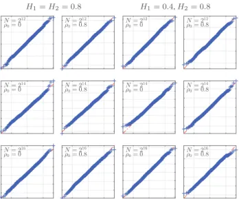
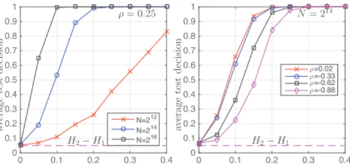
Figure
Documents relatifs