HAL Id: hal-00103291
https://hal.archives-ouvertes.fr/hal-00103291
Submitted on 3 Oct 2006HAL is a multi-disciplinary open access
archive for the deposit and dissemination of sci-entific research documents, whether they are pub-lished or not. The documents may come from teaching and research institutions in France or abroad, or from public or private research centers.
L’archive ouverte pluridisciplinaire HAL, est destinée au dépôt et à la diffusion de documents scientifiques de niveau recherche, publiés ou non, émanant des établissements d’enseignement et de recherche français ou étrangers, des laboratoires publics ou privés.
Controlling chaotic transport in Hamiltonian systems
Guido Ciraolo, Cristel Chandre, Ricardo Lima, Michel Vittot, Philippe
Ghendrih, Marco Pettini
To cite this version:
Guido Ciraolo, Cristel Chandre, Ricardo Lima, Michel Vittot, Philippe Ghendrih, et al.. Controlling chaotic transport in Hamiltonian systems. Physics AUC, 2005, Romania. pp.38-44. �hal-00103291�
Controlling chaotic transport in Hamiltonian systems
Guido Ciraolo∗
Facolt`a di Ingegneria, Universit`a di Firenze via S. Marta, I-50129 Firenze, Italy
Cristel Chandre†, Ricardo Lima‡, Michel Vittot§
CPT-CNRS, Luminy Case 907, F-13288 Marseille Cedex 9, France
Philippe Ghendrih¶
Association Euratom-CEA, DRFC/DSM/CEA, CEA Cadarache F-13108 St. Paul-lez-Durance Cedex, France
Marco Pettinik
Istituto Nazionale di Astrofisica, Osservatorio Astrofisico di Arcetri Largo Enrico Fermi 5, I-50125 Firenze, Italy
Abstract
With the aid of an original reformulation of the KAM theory, it is shown that a relevant control of Hamiltonian chaos is possible through suitable small perturbations whose form can be explicitly computed. In particular, it is shown that it is possible to control (reduce) the chaotic diffusion in the phase space of a 1.5 degrees of freedom Hamiltonian which models the diffusion of charged test particles in “turbulent” electric fields across the confining magnetic field in controlled thermonuclear fusion devices. Though still far from practical applications, this result suggests that some strategy to control turbulent transport in magnetized plasmas, in particular tokamaks, is conceivable.
It is well known that anomalous, noncollisional, losses of energy and particles in magnetic confinement devices of tokamak type still represent a serious obstacle to the attainement of the fea-sibility proof of controlled thermonuclear fusion, [1]. Anomalous transport, being of noncollisional origin, is currently attributed to the presence of turbulent fluctuations of - mainly - electric field in fusion plasmas. Several years ago, it has been shown that the E × B modeling of the guiding centres motions of charged test particles provides a natural explanation of the diffusion across the confining magnetic field B. In fact the intrinsic chaoticity of the dynamics provides a source of strong diffusion [2]. Moreover, even though somewhat too idealized, these models yield chaotic diffusion coefficients in a fairly good agreement with their experimental counterparts [3].
Now, both the empirically found states of improved confinement in tokamaks, and the possibility of reducing and even suppressing chaos with open-loop parametric perturbations of dissipative systems [4, 5], suggest to investigate the possibility of devising a strategy of control of anomalous-chaotic transport through some smart perturbation acting at the microscopic level of charged particles motions. The mentioned models, however, are Hamiltonian and controlling chaos in these models is rather problematic because no attracting sets exist in their phase space.
∗e-mail: [email protected] †e-mail: [email protected] ‡e-mail: [email protected] §e-mail: [email protected] ¶[email protected] ke-mail: [email protected]
However, as it is shown in the present paper, also chaotic Hamiltonian dynamics can be con-trolled. The central idea and meaning of “control” is that one aims at inducing a relevant change in the dynamics (for example reducing or suppressing chaos) by means of a small perturbation (either open- or closed-loop) so that the original structure of the system under investigation is substantially kept unaltered.
In the case of dissipative systems, an efficient strategy of control works by stabilizing unstable periodic orbits where the dynamics is eventually attracted, whereas – at present – for Hamiltonian systems the only hope seems that of looking for a small perturbation, if any, making the system integrable or closer to integrability. In what follows we show that this is actually possible. First we briefly describe the 1.5 degrees of freedom Hamiltonian modeling the E × B motions of charged particles in a “spatially turbulent” electric field, then we sketch a new formulation of the KAM theory due to one of us ([6]) which is to be used to work out a controlling perturbation. Finally, we report the numerical evidence of the effectiveness of the method.
Let us begin by describing the model whose dynamics we want to control. In the guiding centres approximation, the equations of motion of charged particles in presence of a strong toroidal magnetic field and of a nonstationary electric field are
˙x = d dt µx y ¶ = c B2E(x, t) × B = c B µ −∂yV (x, y, t) ∂xV (x, y, t) ¶ (1) where V is the electrostatic potential, E = −∇V , and B = Bez. To define a model we choose
V (x, t) =X
k
Vk. sin[k · x + ϕk− ω(k)t] (2)
where ϕk are random phases and Vk decrease as a given function of k, in agreement with
experi-mental data [7]. In principle one should use for ω(k) the dispersion relation for electrostatic drift waves (which are thought to be responsible for the observed turbulence) with a frequency broaden-ing for each k in order to model the experimentally observed spectrum S(k, ω). Unfortunately this would be prohibitive from a computational point of view, therefore one is led to simplify the model drastically by choosing the phases ϕk at random (with the reasonable hope that the properties of the realization thus obtained are not significantly different from their average). In addition we take for |Vk|2 a power law in |k| to reproduce the spatial spectral characteristics of the experimental S(k), see [7]. And we approximate ω(k) by a constant which we can normalize to 2π, and normalize the coordinates x, y such that their amplitude is 1. Thus we consider the following explicit form of the electrostatic potential
V (x, y, t) = N X m,n=1 a. sin [2π(nx + my + ϕnm− t)] 2π(n2+ m2)3/2 (3)
The spatial coordinates x and y play the role of the canonically conjugated variables. We extend the phase space (x, y) into (E, τ, x, y) where the new dynamical variable τ evolves as: τt = τ0+ t
and E is its canonical conjugate. If we absorb the constant c/B of (1) in the amplitude a, we can consider small values of a, when B is large.
The Hamiltonian of the model is ˜
H(E, τ, x, y) = E + V (x, y, τ ) (4)
and the equations of motion are
˙τ = 1 ˙x = ∂ ˜H ∂y = ∂V ∂y ˙y = − ∂ ˜H ∂x = − ∂V ∂x (5)
Let us now briefly sketch a reformulation of the KAM theory due to one of us [6]. We consider the algebra A “of observables”, i.e. real functions defined on the phase space and we define, for any observable H, a derivation {H} as the Poisson bracket with H. In particular, we consider an integrable hamiltonian H, i.e. such that there exist canonical coordinates (A, θ) with H(A, θ) = H(A). Our problem is to find a relation between the flow generated by a perturbation of H, denoted by ˜H = H + V for some V ∈ A, and the flow of H. More precisely our strategy is to modify the perturbed Hamiltonian ˜H by adding a “small” term f (V ) in order to find a relation between the flow of H + V + f (V ) and the flow of H. The term f (V ) will be called the “control term”. Let us assume that there exists a linear operator N : A → A such that
Γ ≡ (ω(A) · ∂θ)−1N (6)
is well defined, and such that {H}R = 0, where ω(A) ≡ ∂H/∂A and R ≡ (1 − N ). We also define F : A → A by F (V ) ≡ e−{ΓV }(RV ) + 1 − e −{ΓV } {ΓV } (N V ) (7) as well as f : A → A by f (V ) ≡ F (V ) − V (8)
A theorem of [6] stipulates that ∀t ∈ R
et{H+V +f (V )} = e−{ΓV }· et{H}· et{RV }· e{ΓV } (9) The formula (9) connects the perturbed flow, modified by a control term, with the unperturbed flow. The remarkable fact is that the flow of RV commutes with that of H, since {H}R = 0. This allows the splitting of the flow of H + RV into a product. Therefore in the non resonant case (or when RV = 0), H + V + f (V ) is integrable.
Coming to the application to our Hamiltonian (4), we take H(E, x, y, τ ) = E, i.e. independent of x, y, τ , so that A = (E, x) and θ = (τ, y) are action-angle coordinates for H (y can be considered as an angle but it is frozen by the flow of H). We could have exchanged the role of x and y. We have ω(A) = (∂H∂E;∂H∂x) = (1; 0), that is H is resonant. Then ∂θ = (∂τ, ∂y)T and so
{H} = ω(A) · ∂θ = (1, 0).(∂τ, ∂y)T = ∂τ from which Γ = (∂τ)−1N , with R ≡H dτ is the average
over the “time” τ . In our case V is given by the expression (3) and so RV = 0. Now we have all the ingredients in order to compute the control term, given by [6]
f (V ) = ∞ X p=2 fp = (10) X k,n,m∈Z ˜ ǫn,m,k. sin£2π(nx + my + ˜ϕnm+ kτ ) ¤
where the fp are defined to be proportional to ap and the coefficients ˜ǫn,m,kare given in an explicit
form in [6]. Hence if we add the exact expression of the control term to ˜H, the effect on the flow is the confinement of the particle motion, i.e. the fluctuations of the trajectories of the particles, around their initial positions, are uniformly bounded for any time. Moreover it is also shown, in [6] that if we only add an approximation of the exact control term to the potential the effect is still to slow down the diffusion. Therefore, we have computed the first term of the series of the exact control term, f2(x, y, τ ) = − 1 2{ΓV, V } = (11) X n1,m1,n2,m2 a2.(n 2m1− n1m2) ¡(n2 1+ m21)(n22+ m22) ¢3/2 · · sin£2π¡(n1− n2)x + (m1− m2)y + ϕn1m1− ϕn2m2 ¢¤
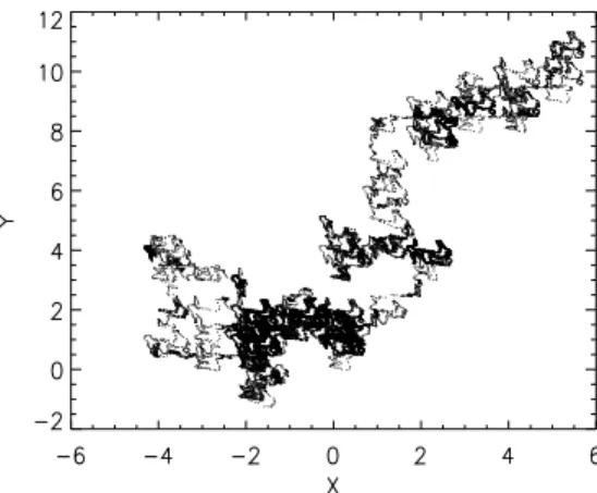
Figure 1: Poincar´e surface of section of a trajectory obtained from the starting Hamiltonian (4) assuming a = 0.8 (weakly chaotic region).
Figure 2: Poincar´e surface of section of a trajectory obtained from the same initial condition as in figure 1 and adding to the starting Hamiltonian the control term (11).
where we have used the explicit form of the coefficients ˜ǫn,m,k. We note that for the particular
model (3), (4) f2 is independent of time.
With the aid of numerical simulations, we check the effectiveness of the above given approach by comparing the diffusion properties of the particle trajectories obtained from Hamiltonian (4) and from the same Hamiltonian with control term (11). Figures 1 and 2 show the Poincar´e surfaces of section of two trajectories issuing from the same initial conditions computed without and with the control term respectively. A clear evidence is found of a relevant reduction of the diffusion in presence of the control term (11). In order to study the diffusion properties of the system, we have considered a set of M particles uniformly distributed at random in the domain 0 ≤ x, y ≤ 1 for t = 0. We have computed the mean square displacement hr2(t)i as a function of time
hr2(t)i = 1 M M X i=1 |xi(t) − xi(0)|2 (12)
where xi(t), i = 1, . . . , M is the position of the i-th particle at time t as obtained by integrating Eqs.
Figure 3: Mean square displacement hr2(t)i versus time t in linear-linear scales obtained from the Hamiltonian (4) for three different values of a.
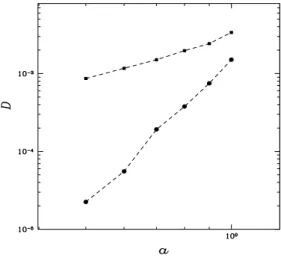
Figure 4: Diffusion coefficient D vs turbulence amplitude parameter a for H given by (4) (full squares) and given by (4) plus the control term (11) (full circles).
diffusion coefficient is derived from
D = lim
t→∞
hr2(t)i
t .
Figure 3 shows hr2(t)i for 3 different values of a. As predicted, the action of the control term
gets weaker as a is increased towards the strongly chaotic phase: see Figure 4. We can check the robustness of the control scheme by replacing f2 by δ.f2 and varying the parameter δ away from its
reference value δ = 1. Figure 5 shows that both the increase and the reduction of the magnitude of the control term (which is proportional to δ.a2) results in a loss of efficiency in reducing the diffusion coefficient. The fact that a larger perturbation term – with respect to the computed one – does not work better, also means that the perturbation is “smart” and that it is not a “brute force” effect. Let us define the “horizontal (resp. vertical) step size” as the distance covered by the test particle between two successive sign reversals of the horizontal (resp. vertical) component of the drift velocity. The effect of the control perturbation is analysed in terms of the Probability Distribution Function (PDF) of step sizes. Following test particle trajectories for a large number of initial conditions, with and without control, leads to the PDFs plotted on Figure 6. A marked
Figure 5: Diffusion coefficient D vs magnitude of the control term (11) for the fixed value of a = 0.7 10-4 10-3 10-2 10-1 PDF 1.2 0.8 0.4 0.0 step size without control with control
Figure 6: PDF of the magnitude of the horizontal step size with and without the control pertur-bation.
reduction of the PDF is observed at large step sizes “with control” relatively to the “no control” case. Conversely, an increase is found for the smaller step size. The control procedure thus appears to quench the large steps, typically larger than 0.5. In order to measure the relative magnitude between the hamiltonian (4) and f2, we have numerically computed their mean squared values. We
have considered 105 random initial conditions in the xy square [0, 1] × [0, 1] for 100 different times. And we find that:
s hf2
2i − hf2i2
hV2i − hV i2 ≈ 0.01a (13)
This means that the control term can be considered as a small perturbative term.
So to conclude this work, we have provided an effective new stategy to control the chaotic diffusion in Hamiltonian dynamics using a small perturbation. We also compared the result of an optimal control with the corresponding one for an approximate control. Since the formula for the control term is explicit, we are able to compare the dynamics without and with control in a simplified model, describing anomalous electrostatic transport in magnetized plasmas. Even
though we use a rather simplified model to describe anomalous transport of charged particles in fusion plasmas, our result makes it conceivable that to apply some smart perturbation could lead to a relevant reduction of the anomalous losses of energy and particles in tokamaks.
References
[1] W. Horton, Rev. Mod. Phys. 71, 735 (1999). [2] M. Pettini et al., Phys. Rev. A38, 344 (1988).
[3] M. Pettini: Low Dimensional Hamiltonian Models for Non-Collisional Diffusion of Charged Particles, in “Non-Linear Dynamics” (Bologna, May 1988), G. Turchetti Ed., World Scientific, Singapore (1989) 287-296.
[4] R. Lima and M. Pettini, Phys. Rev. A41, 726 (1990); Int. J. Bif. & Chaos 8, 1675 (1998); L. Fronzoni, M. Giocondo, M. Pettini, Phys. Rev.A43, 6483 (1991).
[5] G. Chen and X. Dong, Int. J. Bif. & Chaos, 3, 1363 (1993).
[6] M. Vittot: “Perturbation Theory and Control in Classical or Quantum Mechanics by an Inversion Formula”, J. Phys. A: Math. Gen. vol 37 (2004) p 6337. Archived in math-ph/0303051 or mp-arc/03-147, (2003)