HAL Id: hal-00426563
https://hal.archives-ouvertes.fr/hal-00426563v2
Submitted on 28 Jun 2010
HAL is a multi-disciplinary open access
archive for the deposit and dissemination of
sci-entific research documents, whether they are
pub-lished or not. The documents may come from
teaching and research institutions in France or
abroad, or from public or private research centers.
L’archive ouverte pluridisciplinaire HAL, est
destinée au dépôt et à la diffusion de documents
scientifiques de niveau recherche, publiés ou non,
émanant des établissements d’enseignement et de
recherche français ou étrangers, des laboratoires
publics ou privés.
The Area Method : a Recapitulation
Predrag Janicic, Julien Narboux, Pedro Quaresma
To cite this version:
Predrag Janicic, Julien Narboux, Pedro Quaresma. The Area Method : a Recapitulation. Journal
of Automated Reasoning, Springer Verlag, 2012, 48 (4), pp.489-532. �10.1007/s10817-010-9209-7�.
�hal-00426563v2�
(will be inserted by the editor)
The Area Method
A Recapitulation
Predrag Janiˇci´c · Julien Narboux · Pedro Quaresma
Received: 2009/10/07 / Accepted:
Abstract The area method for Euclidean constructive geometry was proposed by Chou, Gao and Zhang in the early 1990’s. The method can efficiently prove many non-trivial ge-ometry theorems and is one of the most interesting and most successful methods for auto-mated theorem proving in geometry. The method produces proofs that are often very concise and human-readable.
In this paper, we provide a first complete presentation of the method. We provide both algorithmic and implementation details that were omitted in the original presentations. We also give a variant of Chou, Gao and Zhang’s axiom system. Based on this axiom system, we proved formally all the lemmas needed by the method and its soundness using the Coq proof assistant.
To our knowledge, apart from the original implementation by the authors who first pro-posed the method, there are only three implementations more. Although the basic idea of the method is simple, implementing it is a very challenging task because of a number of details that has to be dealt with. With the description of the method given in this paper, implement-ing the method should be still complex, but a straightforward task. In the paper we describe all these implementations and also some of their applications.
Keywords area method· geometry · automated theorem proving · formalisation Mathematics Subject Classification (2000) 51A05· 68T15
The first author is partially supported by a grant 144030 of the Ministry of Science of Serbia. The second author is partially supported by the ANR project Galapagos.
Predrag Janiˇci´c
Faculty of Mathematics, University of Belgrade Studentski trg 16, 11000 Belgrade, Serbia E-mail: [email protected]
Julien Narboux
LSIIT, UMR 7005 CNRS-ULP, University of Strasbourg Pˆole API, Bd S´ebastien Brant, BP 10413, 67412 Illkirch, France E-mail: [email protected]
Pedro Quaresma
CISUC, Department of Mathematics, University of Coimbra 3001-454 Coimbra, Portugal
1 Introduction
There are two major families of methods in automated reasoning in geometry: algebraic style and synthetic style methods.
Algebraic style has its roots in the work of Descartes and in the translation of geo-metric problems to algebraic problems. The automation of the proving process along this line began with the quantifier elimination method of Tarski [59] and since then had many improvements [15]. The characteristic set method, also known as Wu’s method [4, 63], the elimination method [62], the Gr¨obner basis method [35, 36], and the Clifford algebra ap-proach [39] are examples of practical methods based on the algebraic apap-proach. All these methods have in common an algebraic style, unrelated to traditional, synthetic geometry methods, and they do not provide human-readable proofs. Namely, they deal with polyno-mials that are often extremely complex for a human to understand, and also with no direct link to the geometrical contents.
The second approach to the automated theorem proving in geometry focuses on syn-thetic proofs, with an attempt to automate the traditional proving methods. Many of these methods add auxiliary elements to the geometric configuration considered, so that a certain postulates could apply. This usually leads to a combinatorial explosion of the search space. The challenge is to control the combinatorial explosion and to develop suitable heuristics in order to avoid unnecessary construction steps. Examples of synthetic proof methods in-clude approaches by Gelertner [20], Nevis [48], Elcock [18], Greeno et al. [23], Coelho and Pereira [14], Chou, Gao, and Zhang [8].
In this paper we focus on the area method, an efficient coordinates-free method for a fragment of Euclidean geometry, developed by Chou, Gao, and Zhang [8, 9, 11] that is somewhere between the two above styles. This method enables one to implement provers capable of proving many complex geometry theorems. The method is sometimes credited (e.g., by its authors) to produce traditional, human-readable proofs. The generated proofs are indeed often concise, consisting of steps that are directly related to the geometrical contents involved and hence can be readable and easily understood by a mathematician. However, since the proofs are formulated in terms of arithmetic expressions, they can also significantly differ from traditional, Hilbert-style, synthetic proofs given in textbooks. Also, proofs may involve huge expressions, hardly readable, despite the fact their atomic expressions have clear and intuitive geometrical meaning.
The main idea of the area method is to express the hypotheses of a theorem using a set of starting (“free”) points and a set of constructive statements each of them introducing a new point, and to express the conclusion by an equality between polynomials in some geometric quantities (without considering Cartesian coordinates). The proof is developed by eliminating, in reverse order, the points introduced before, using for that purpose a set of appropriate lemmas. After eliminating all the introduced points, the goal equality of the conjecture collapses to an equality between two rational expressions involving only free points. This equation can be further simplified to involve only independent variables. If the expressions on the two sides are equal, the conjecture is a theorem, otherwise it is not. All proof steps generated by the area method are expressed in terms of applications of high-level geometry lemmas and expression simplifications.
Although the basic idea of the method is simple, implementing it is a very challenging task because of a number of details that has to be dealt with. To our knowledge, apart from the original implementation by the authors who first proposed the area method, there are only three other implementations. These three implementations were made independently and in different contexts:
– within a tool for storing and exploring mathematical knowledge (Theorema [2]) — im-plemented by Judit Robu [58].
– within a generic proof assistant (Coq [61]) — implemented by Julien Narboux [43]; – within a dynamic geometry tool (GCLC [29]) — implemented by Predrag Janiˇci´c and
Pedro Quaresma [33];
The implementations of the method can efficiently find proofs of a range of non-trivial theorems, including theorems due to Ceva, Menelaus, Gauss, Pappus, and Thales.
In this paper, we present an in-depth description of the area method covering all relevant definitions and lemmas. We also provide some of the implementation details, which are not given or not clearly stated in the original presentations. We follow the original exposition, but in a reorganised, more methodological form. This description of the area method should be sufficient for a complete understanding of the method, and for making a new imple-mentation a straightforward task. This paper also summarises our results, experiences, and descriptions of our software systems related to the area method [30, 33, 43, 45, 52, 54].
In this paper we consider only the basic variant of the area method for Euclidean geom-etry, although there are other variants. Additional techniques can also be used to produce shorter proofs and slightly extend the basic domain of the method [9]. However, these tech-niques are applicable only in special cases and not in a uniform way, in contrast to the basic method. It is also possible to extend the area method to deal with goals in the form of in-equalities (of the form L< R or L ≤ R). In that case, the inequality can be decided using an CAD algorithm or a heuristic like the sum of squares method. There are also variants of the area method developed for solid Euclidean geometry [10] and for hyperbolic plane geom-etry [64]. Substantially, the main idea of these variants is the same as in the basic method and this demonstrates that the approach has a wide domain. Variants of the method can be implemented in the same way described in this paper.
Overview of the paper.The paper is organised as follows: first, in Section 2, we explain the area method in details. In Section 3, we describe all the existing implementations of the method and some of their applications. In Section 4 we summarise our contributions and we draw final conclusions in Section 5.
2 The Area Method
The area method is a decision procedure for a fragment of Euclidean plane geometry. The method deals with problems stated in terms of sequences of specific geometric construction steps. We begin introducing the method by way of example.
In the rest of the paper, capital letters will denote points in the plane and△ABC will denote the triangle with vertices A, B, and C.
2.1 Introductory Example
The following simple example briefly illustrates some key features of the area method. Example 2.1 (Ceva’s Theorem) Let△ABC be a triangle and P be an arbitrary point in
the plane. Let D be the intersection of AP and BC, E be the intersection of BP and AC, and F the intersection of CP and AB. Then:
AF FB BD DC CE EA= 1
This result can be stated and proved, within the area method setting.
The Construction.The points A, B, C, and P are free points, points not defined by construc-tion steps. The point D is the intersecconstruc-tion of the line determined by the points A and P and of the line determined by the points B and C. The points E and F are constructed in a similar fashion.
For this problem, an initial non-degeneracy condition is that it holds F6= B, D 6= C, and
E6= A. Notice also that the point P is not completely arbitrary point in the plane, since it should not belong to the three lines parallel to the sides of the triangle and passing through the opposite vertices (Figure 2.1).
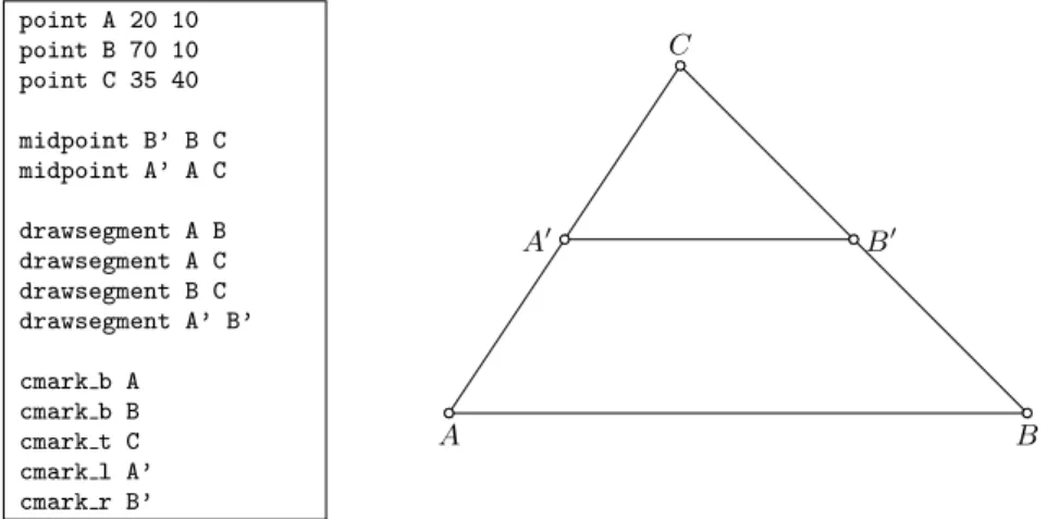
A B C D F E P
Fig. 2.1 Illustration for Ceva’s theorem
Stating the Conjecture.One of the key problems in automated theorem proving in geometry is the control of the combinatorial explosion that arises from the number of similar, but still different, cases that have to be analysed. For instance, given three points A, B, and C, how many triangles do they define? One can argue that the answer is one, but from a syntactic point of view,△ABC is not equal to △ACB. For reducing such combinatorial explosion, but also for ensuring rigorous reasoning, one has to deal with arrangement relations, such as on the same side of a line, two triangles have the same orientation, etc. Note that, in Euclidean geometry, positive and negative orientation are just two names used to distinguish between the two orientations and one can select any triangle in the plane and proclaim that it has the orientation that will be called positive (and it is similar with orientation of segments on a line). In other words, in Euclidean geometry the notion of orientation is relative rather then absolute, and one can prove that a triangle has positive orientation, only if positive (and negative) orientation was already defined via some triangle in the same plane. In the Cartesian model of Euclidean geometry, the two orientations are distinguished as clockwise and counterclockwise orientations. These two names should not be used for
Euclidean geometry, because they cannot be defined there. Unfortunately, these terms are widely used in geometrical texts, including in the description of the area method [67].
For stating and proving conjectures, the area method uses a set of specific geometric
quantitiesthat enable treating arrangement relations. Some of them are:
– ratio of parallel directed segments, denoted AB/CD. If the points A, B, C, and D are collinear, AB/CD is the ratio between lengths of directed segments AB and CD. If the points A, B, C, and D are not collinear, and it holds ABkCD, there is a parallelogram
ABPQsuch that P, Q, C, and D are collinear and thenCDAB =CDQP.
– signed area for a triangle ABC, denotedSABCis the area of the triangle ABC, negated if
ABChas the negative orientation. – Pythagoras difference,1denotedP
ABC, for the points A, B, C, defined asPABC= AB2+
CB2− AC2.
These three geometric quantities allow expressing (in form of equalities) geometry prop-erties such as collinearity of three points, parallelism of two lines, equality of two points, perpendicularity of two lines, etc. (see section 2.2.1). In the example, the conjecture is ex-pressed using ratios of parallel directed segments.
Proof.The proof of a conjecture is based on eliminating all the constructed points, in reverse order, using for that purpose the properties of the geometric quantities, until an equality in only the free points is reached. If the equality is provable, then the original conjecture is a theorem as well. For the given example, a proof can be as follows:
It can be proved thatAFFB=SAPC
SBCP. By analogy BD DC= SBPA SCAP and CE EA= SCPB SABP. Therefore: AF FB BD DC CE EA = SAPC SBCP BD DC CE
EA the point F is eliminated = SAPC
SBCP SBPA SCAP
CE
EA the point D is eliminated = SAPC
SBCP SBPA SCAP
SCPB
SABP the point E is eliminated
= 1
Q.E.D. The example illustrates how to express a problem using the given geometric quantities and how to prove it, and moreover, how to give a proof that is concise and very easy to understand.
The complete proof procedure will be given in Section 2.5. Before that, the underlying axiom system will be introduced.
2.2 Axiomatic Grounds for the Area Method
There is a number of axiom systems for Euclidean geometry. Euclid’s system [26], partly naive from today’s point of view, was used for centuries. In the early twentieth century, Hilbert provided a more rigorous axiomatisation [27], one of the landmarks for modern
1 The Pythagoras difference is a generalisation of the Pythagoras equality regarding the three sides of a
right triangle, to an expression applicable to any triangle (for a triangle ABC with the right angle at B, it holds that PABC= 0).
property in terms of geometric quantities points A and B are identical PABA= 0
points A, B, C are collinear SABC= 0
ABis perpendicular to CD PABA6= 0 ∧ PCDC6= 0 ∧ PACD= PBCD
ABis parallel to CD PABA6= 0 ∧ PCDC6= 0 ∧ SACD= SBCD
Ois the midpoint of AB SABO= 0 ∧ PABA6= 0 ∧AOAB=12
ABhas the same length as CD PABA= PCDC
points A, B, C, D are harmonic SABC= 0 ∧ SABD= 0 ∧ PBCB6= 0 ∧ PBDB6= 0 ∧ACCB=DADB
angle ABC has the same measure as DEF PABA6= 0∧PACA6= 0∧PBCB6= 0∧PDED6= 0∧PDFD6= 0∧
PEFE6= 0∧ SABC· PDEF= SDEF· PABC
Aand B belong to the same circle arc CD SACD6= 0 ∧ SBCD6= 0 ∧ SCAD· PCBD= SCBD· PCAD
Table 2.1 Expressing geometry predicates in terms of the three geometric quantities.
mathematics, but still not up to modern standards [16, 42]. In the mid-twentieth century, Tarski presented a new axiomatisation for elementary geometry (with a limited support for continuity features), along with a decision procedure for that theory [60]. Although there are other variations of these systems [31, 44], these three are the most influential and most popular axiomatic systems for geometry.
Modern courses on classical Euclidean geometry are most often based on Hilbert’s ax-ioms. In Hilbert-style geometry, the primitive (not defined) objects are: point, line, plane. The primitive (not defined) predicates are those of congruence and order (with addition of equality and incidence2). Properties of the primitive objects and predicates are introduced by five groups of axioms, such as: “For two points A, B there exists a line a such that both A and B are incident with it”.
In the following text we briefly discuss how axiomatic grounds can be built for the fragment of geometry treated by the area method.
2.2.1 A Hilbert Style Axiomatisation
The geometric quantities used within the area method (mentioned in Section 2.1) can be defined in Hilbert style geometry, but they also require axioms of the theory of fields. The notions of the ratio of parallel directed segments and of the signed area involve the notion of orientation of segments on a line and the notion of orientation of triangles in a plane (discussed in section 2.1).
Using geometric quantities, it is possible to express a range of geometry predicates as shown in Table 2.1.
The given correspondences can be proved as theorems of Hilbert’s geometry. For in-stance, one direction of the property about angle congruence can be proved as follows. Since A, B, and C define an angle, they are different by definition (i.e.,PABA6= 0,PACA6= 0,
PBCB6= 0), and the same holds for the points D, E, F. If the angle ABC is a right angle, then
PABC=PDEF= 0 and triviallySABC·PDEF =SDEF·PABC; otherwise, by the cosine rule,
SABC/PABC= (12AB· BC · sin(ABC))/(AB2+ CB2− (AB2+ CB2− 2AB · BC cos(ABC))) = sin(ABC)/(4 cos(ABC)) = tan(ABC)/4; hence, if the angle DEF is congruent to ABC, then
SABC/PABC= tan(ABC)/4 =SDEF/PDEF and, furtherSABC·PDEF=SDEF·PABC. Proofs generated by the area method use a set of specific lemmas (see Section 2.4). These lemmas can be proved within Hilbert’s geometry (i.e., within its fragment for plane
geometry), but the full, formal proofs would be very long and would involve complex no-tions like orientation and area of a triangle. That is why it is suitable to have an alternative, higher-level axiomatisation, suitable for the area method. Chou, Gao and Zhang [8] pro-posed such a system for affine geometry, and in the next section we propose a variant of this system.
2.2.2 A New Axiom System for the Area Method
The axiom system used by Chou, Gao and Zhang [8, 9] is a semi-analytic axiom system with (only) points as primitive objects (lines are not primitive objects as in Hilbert’s axiom system). The axiom system contains the axioms of field, so the system uses the concept of numbers, but it is still coordinate free. The field is not assumed to be ordered, hence the axiom system has the property of representing an unordered geometry. This means that, for instance, one cannot express the concept of a point being between two points (unlike in Hilbert’s system).
In the following, we present our special-purpose axiom system for Euclidean plane ge-ometry (within first order logic with equality), a modified version of the axiomatic system of Chou, Gao and Zhang.
In contrast to Hilbert’s system, in our axiom system there is just one primitive type of geometrical objects: points. Variables can also range over a field(F, +, ·,0,1). F is any field of characteristic different from 2.3The axioms of the theory of fields are standard and hence omitted.
There is one primitive binary function symbol (··) and one ternary function symbols (S...) from points to F. The first depicts the signed distance between two points, the second
represents the signed area of a triangle. All axioms given in Table 2.2 are implicitly univer-sally quantified. To improve readability (of the last three axioms), the following shorthands are used: PABC ≡ AB 2 + BC2− AC2 ABk CD ≡ SACD=SBCD AB⊥ CD ≡ PACD=PBCD
The following shorthands are also used within the method for better readability:
SABCD ≡ SABC+SACD
PABCD≡PABD−PCBD
Definition 2.1 (Geometry Quantities) Geometry quantities are expressions of the formAB CD,
SABC,SABCD,PABC,PABCD.
Relationship with the Hilbert style geometry. Note that in the Hilbert style approach, pred-icates··,S..., andP...and are all defined (see Section 2.2.1), while in this approach,··,S...
are primitive predicates andP...is a defined predicate. In both cases, ratio of parallel
di-rected segments is defined using the notions of the theory of fields. Provable properties of Hilbert’s geometry shown in Table 2.1, can be used as definitions (for notions of parallel lines, perpendicular lines, etc) in the area method theory. Thanks to all these definitions, all
3 The fact that the characteristic of F is different from 2 is used to simplify the axiom system. Indeed,
if 06= 2 since ∀ABC,SABC= −SBAC(by axiom 3) then∀AC,SAAC= −SAACand hence∀AC,SAAC= 0, so
we can omit the axiom SAAC= 0 which appears in the system proposed by Chou et al. In addition, this
assumption allows, for instance, construction of the midpoint (using the construction axiom with r=1 2) of a
1. AB= 0 if and only if the points A and B are identical 2. SABC= SCAB
3. SABC= −SBAC
4. If SABC= 0 then AB + BC = AC (Chasles’s axiom)
5. There are points A, B, C such that SABC6= 0 (dimension; not all points are collinear)
6. SABC= SDBC+ SADC+ SABD(dimension; all points are in the same plane)
7. For each element r of F, there exists a point P, such that SABP= 0 and AP = rAB (construction of a point
on the line)
8. If A6= B,SABP= 0, AP = rAB, SABP′= 0 and AP′= rAB, then P = P′(unicity) 9. If PQk CD andPQ
CD= 1 then DQ k PC (parallelogram)
10. If SPAC6= 0 and SABC= 0 thenABAC=
SPAB
SPAC (proportions)
11. If C6= D and AB ⊥ CD and EF ⊥ CD then AB k EF 12. If A6= B and AB ⊥ CD and AB k EF then EF ⊥ CD 13. If FA⊥ BC and SFBC= 0 then 4SABC2 = AF
2
BC2(area of a triangle) Table 2.2 The axiom system
well-formed formulae of the theory of the area method are also well-formed formulae of the Hilbert style geometry. Moreover, all presented axioms of the area method can be proved in the Hilbert style geometry as theorems.4Because of that, each conjecture that can be proved
by the axioms for the area method, is also a theorem of Hilbert’s geometry (assuming the same inference system).
Relationship with the axiom system of Chou, Gao, and Zhang. Our axiom system is an ex-tended and modified version of the original system by Chou, Gao, and Zhang. While their axiom system deals with affine geometry only (and does not introduce the notion of Pythago-ras difference), our system contains axioms about PythagoPythago-ras difference (axioms 11, 12, and 13) and, thanks to that, deals with Euclidean geometry. Compared to the original ver-sion, ours has also the advantage of being more precise and organised. The axiom system we propose differs from the axiom system of Chou, Gao and Zhang in the following ways too:
1. Our system does not use collinearity as a primitive notion and instead, collinearity is de-fined by the signed area. Chou, Gao and Zhang’s system has axioms introducing prop-erties of collinearity, and these axioms are then used for proving that three points are collinear if and only ifSABC= 0 [9].
2. While Chou, Gao and Zhang’s axiom system restricts to ratios of directed parallel seg-ments CDAB where the lines AB and CD are parallel, we skip this syntactical restriction and can use ratios for arbitrary points. The consistency of the axiom system is preserved because the concept of oriented distance can be interpreted in the standard Cartesian model. The area method requires explicitly that for every ratio of directed segmentsCDAB,
AB is parallel to CD. Therefore, the area method is not a decision procedure for this theory, as it can not prove or disprove all conjectures stated in the introduced language because the method can not deal with ratios of the form AB
CDif AB∦ CD (however, it is a decision procedure for the set of formulae from the restricted version of the language).
4 We don’t have formal proofs for these conjectures as they would involve formalisation of very complex
notions like orientation and area of a triangle, which is still beyond reach for current formalisation of Hilbert’s geometry.
Finally, using our axiom system — more suitable for that task — we formally verified (within the Coq proof assistant [61]) all the properties of the geometric quantities required by the area method, demonstrating the correctness of the system and eliminating all concerns about provability of the lemmas [47].
2.3 Geometric Constructions
The area method is used for proving constructive geometry conjectures: statements about properties of objects constructed by some fixed set of elementary constructions. In this sec-tion we first describe the set of available construcsec-tion steps and then the set of conjectures that can be expressed.
2.3.1 Elementary Construction Steps
Constructions covered by the area method are closely related, but still different, from con-structions by ruler and compass. These are the elementary concon-structions by ruler and com-pass:
– construction of an arbitrary point; – construction of an arbitrary line;
– construction (by ruler) of a line such that two given points belong to it;
– construction (by compass) of a circle such that its centre is one given point and such that the second given point belongs to it;
– construction of a point such that it is the intersection of two lines (if such a point exists); – construction of the intersections of a given line and a given circle (if such points exists). – construction of the intersections of two given circles (if such points exists).
The area method cannot deal with all geometry theorems involving the above construc-tions. It does not support construction of an arbitrary line, and it supports intersections of two circles and intersections of a line and a circle only in a limited way.
Instead of support for intersections of two circles or a line and a circle (critical for describing many geometry theorems), there are new, specific construction steps. All con-struction steps supported by the area method are expressed in terms of the involved points.5 Therefore, only lines and circles determined by specific points can be used (rather than ar-bitrarily chosen lines and circles) and the key construction steps are those introducing new points. For a construction step to be well-defined, certain conditions may be required. These conditions are called non-degeneracy conditions (ndg-conditions).
In the following text, (LINEU V) will denote a line such that the points U and V belong to it, and (CIRCLEO U) will denote a circle such that its centre is point O and such that the point U belongs to it.
Some of the construction steps are formulated using the fixed field (F, +, ·,0,1), em-ployed by the used axiom system.
5 Elementary construction steps used by the area method do not use the concept of line and plane explicitly.
This is convenient from the point of view of formalisation and automation. Indeed, in an axiom system based only on the concept of points (as in Tarski’s axiom system [60]), the dimension implied can be easily changed by adding or removing some appropriate axioms (stated in the original signature). On the other hand, in an axiom system based on the concepts of points and lines, such as Hilbert’s axiom system, in order to extend the system to the third dimension ones needs both to update some axioms, to introduce some new axioms and to change the signature of the theory by introducing the sort of planes.
Given below is the list of elementary construction steps in the area method, along with the corresponding ndg-conditions. Free points are introduced only by ECS1 and, if r is a variable, by ECS4 and by ECS5.
ECS1 construction of an arbitrary point U; this construction step is denoted by (POINTU). ndg-condition: –
ECS2 construction of a point Y such that it is the intersection of two lines (LINEU V) and (LINEP Q); this construction step is denoted by (INTERY U V P Q).
ndg-condition: UV∦ PQ; U 6= V ; P 6= Q.
A formula that corresponds to this construction step is: U6= V ∧ P 6= Q ∧ UV ∦ PQ ∧
SUVY = 0 ∧SPQY= 0.
ECS3 construction of a point Y such that it is the foot from a given point P to (LINEU V); this construction step is denoted by (FOOTY P U V).
ndg-condition: U6= V
A formula that corresponds to this construction step is: U6= V ∧ PY ⊥ UV ∧SUVY= 0. ECS4 construction of a point Y on the line passing through a point W and is parallel to (LINEU V), such that WY= rUV , where r is an element of F, a rational expression in geometric quantities, or a variable; this construction step is denoted by (PRATIOY W U Vr).
ndg-condition: U 6= V ; if r is a rational expression in the geometric quantities, the de-nominator of r should not be zero.
A formula that corresponds to this construction step is: U6= V ∧WY k UV ∧WY UV = r. ECS5 construction of a point Y on the line passing through a point U and perpendicular to
(LINEU V), such that 4SUVY
PUVU = r, where r is a rational number, a rational expression in
geometric quantities, or a variable; this construction step is denoted by (TRATIOY U V
r).
ndg-condition: U6= V ; if r is a rational expression in geometric quantities then the de-nominator of r should not be zero.
A formula that corresponds to this construction step is: U6= V ∧UY ⊥ UV ∧4SUVY
PUVU = r.
The above set of construction steps is sufficient for expressing many constructions based on ruler and compass, but not all of them. For instance, an arbitrary line cannot be con-structed by the above construction steps. Still, one can construct two arbitrary points and then (implicitly) the line going through these points.
Also, intersections of two circles and intersections of a line and a circle are not supported in a general case. However, it is still possible to construct intersections of two circles and intersections of a line and a circle in some special cases. For example:
– construction of a point Y such that it is the intersection (other than point U) of a line (LINEU V) and a circle (CIRCLEO U) can be represented as a sequence of two con-struction steps: (FOOTN O U V), (PRATIOY N N U-1).
– construction of a point Y such that it is the intersection (other than point P) of a circle (CIRCLEO1 P) and a circle (CIRCLEO2 P) can be represented as a sequence of two construction steps: (FOOTN P O1 O2), (PRATIOY N N P-1).
In addition, many other constructions (expressed in terms of constructions by ruler and compass) can be performed by the elementary constructions of the area method. Some of them are:
– construction of a line such that a given point W belongs to it and it is parallel to a line (LINEU V); such line is determined by the points W and N, where N is obtained by (PRATION W U V1).
– construction of a line such that a given point W belongs to it and it is perpendicular to a line (LINEU V); if W , U , V are collinear, then such line is determined by the points W and N, where N is obtained by (TRATION W U1), otherwise, such line is determined by the points W and N, where N is obtained by (FOOTN W U V).
– construction of a perpendicular bisector of a segment with endpoints U and V ; such line is determined by the points N and M, where these points are obtained by (PRATIOM U U V1/2), (TRATION M U1).
Also, it is possible to construct an arbitrary point Y on a line (LINEU V), by (PRATIOY U U V r) where r is an indeterminate, or on a circle (CIRCLEO P), by (POINTQ), (FOOT N O P Q), (PRATIOY N N P-1). There can be also used some additional construction steps (with corresponding elimination lemmas) that can help producing shorted proofs in some cases [8] but we will not describe them here.
Within a wider system (e.g., within a dynamic geometry tool), a richer set of construc-tion steps can be used for describing geometry conjectures as long as all of them can be represented by the elementary construction steps of the area method.
As said, the set of elementary construction steps in the area method cannot cover all constructions based on ruler and compass. On the other hand, there are also some construc-tions that can be performed by the above construction steps and that cannot be performed by ruler and compass. For instance, if√32∈ F then, given two distinct points A and B, one can construct a third point C such that AC=√3
2 AB, since one can use this number (whereas it is not possible using ruler and compass).
Example 2.2 The construction given in Example 2.1 can be represented in terms of the
given construction steps as follows: A, B,C, P are free points (ECS1)
(INTERD A P B C) (ECS2)
(INTERE B P A C) (ECS2)
(INTERF C P A B) (ECS2)
2.3.2 Constructive Geometry Statements
In the area method, geometry statements have a specific form.
Definition 2.2 (Constructive Geometry Statement) A constructive geometry statement, is
a list S= (C1,C2, . . . ,Cm, G) where Ci, for1≤ i ≤ m, are elementary construction steps, and
the conclusion of the statement, G is of the form E1= E2, where E1and E2are polynomials in geometric quantities of the points introduced by the steps Ci. In each of Ci, the points used
in the construction steps must be already introduced by the preceding construction steps.
The class of all constructive geometry statements is denoted by C.
Note that, in its basic form, the area method does not deal with conclusion statements in the form of inequalities (for another variants of the method see Section 2.5.8 and Sec-tion 3.3.2).
For a statement S= (C1,C2, . . . ,Cm, (E1= E2)) from C, the ndg-condition is the set of
the ndg-conditions of the steps Ci, plus the conditions dithat the denominators appearing in E1 and E2 are not equal to zero, and the conditions pithat lines appearing in ratios of segments in E1and E2are parallel: for each ratio of the form CDAB appearing in E1 and E2,
c1∧ c2∧ ... ∧ cm∧
d1∧ ... ∧ dm∧
p1∧ ... ∧ pm∧ ⇒ E1= E2
where ciare the formulae characterising the construction steps (including their ndg-conditions). The formula above is assumed to be universally quantified.
The area method (as described in this paper) decides whether or not a conjecture of the above form is a theorem, i.e., whether it can be derived from the axiom system described in Section 2.2.2. If a conjecture is a theorem in the theory of the area method, then it is also a theorem of the Hilbert style geometry (as discussed in Section 2.2.2). Note that the area method is applied for statements of the form H⇒ E1= E2, while definitions of some
geometry properties may involve inequalities as well, for instance, we say that AB is parallel
to CDifPABA6= 0 ∧PCDC6= 0 ∧SACD=SBCD. Typically, when proving properties defined in Table 2.1, instead of provingPABA6= 0 ∧PCDC6= 0 ∧SACD=SBCD, the method is applied only for provingSACD=SBCD, which gives a weaker conjecture (for the special cases of
A= B and C = D). Adding A 6= B and C 6= D to the set of ndg-conditions, would ensure that
these two goals are equivalent.
Example 2.3 The statement corresponding to the theorem given in Example 2.1 can be
represented as follows: A6= P ∧ B 6= C ∧ AP ∦ BC ∧SAPD= 0 ∧SBCD= 0 ∧ B6= P ∧ A 6= C ∧ BP ∦ AC ∧SBPE= 0 ∧SACE= 0 ∧ C6= P ∧ A 6= B ∧CP ∦ AB ∧SCPF= 0 ∧SABF= 0 ∧ F6= B ∧ D 6= C ∧ E 6= A ∧ AFk FB ∧ BD k DC ∧CE k EA ⇒ AF FB BD DC CE EA= 1
2.4 Properties of Geometric Quantities and Elimination Lemmas
We present some definitions and the properties of geometric quantities, required by the area method. We follow the material from original descriptions of the method [8, 9, 11, 67], but in a reorganised form. The rigorous traditional proofs (not formal) in the Hilbert’s style geometry, accompanying all the results presented in this section are available [56]. The formal (machine verifiable) proofs are available as a Coq contribution [47].
The following lemmas are implicitly universally quantified and it is assumed that it holds
A6= B for any ratio of parallel directed segments of the formXYAB. Lemma 2.1 PQAB= −QP AB= QP BA= − PQ BA. Lemma 2.2 PQAB= 0 iff P = Q. Lemma 2.3 PQ AB AB PQ= 1.
Lemma 2.4 SABC=SCAB=SBCA= −SACB= −SBAC= −SCBA. Lemma 2.5 PAAB= 0.
Lemma 2.6 PABC=PCBA. Lemma 2.7 PABA= 2AB
2 . 2.4.1 Elimination Lemmas
An elimination lemma is a theorem that has the following properties:
– it states an equality between a geometric quantity involving a certain constructed point
Yand an expression not involving Y ;
– this last expression is composed using only geometric quantities;
– this expression is well defined: denominators are different from zero and ratios of seg-ments are composed only using parallel segseg-ments.
It is required to describe elimination of points introduced by four construction steps (ECS2 to ECS5) from three kinds of geometric quantities.
Some elimination lemmas enable eliminating a point from expressions only at certain positions — usually the last position in the list of the arguments. That is why it is necessary first to transform relevant terms of the current goal into the form that can be dealt with by these elimination lemmas. Moreover, some elimination lemmas require that some points are assumed to be distinct. The first following lemma ensures that this assumptions can be met. Lemma 2.8 If G is a geometric quantity involving Y , then either G is equal to zero or it can
be transformed into one of the following forms (or their sum or difference), for some A, B, C, and D that are different from Y :
AY CD; AY BY;− AY BY; 1 AY CD ;PABY;PAY B;SABY
Proof: If G is a geometric quantity of arity 4 (SABCD orPABCD), the first step is to trans-form it into terms of arity 3, using the shorthands defined in section 2.2.2:SABCD≡SABC+
SACD,PABCD≡PABD−PCBD.
Now, all remaining geometric quantities (involving Y ) can be treated.
Signed ratios: G can have one of the following forms (for some A, B, and C different from
Y): • YYAY = 0 (by Lemma 2.2) • YY YA = 0 (by Lemma 2.2) • YY CD= 0 (by Lemma 2.2) • AY BY • AY Y B= − AY BY (by Lemma 2.1) • YA BY = − AY BY (by Lemma 2.1) • YA Y B= AY BY (by Lemma 2.1) • AY CD • YA CD= − AY CD (by Lemma 2.1) • AB CY = 1 CY AB
(by lemmas 2.1 and 2.3) • YCAB= CY1
BA
Signed area: G can have one of the following forms (for some A and B different from Y ): • SYYY= 0 (by Lemma 2.4)
• SAYY= 0 (by Lemma 2.4) • SYAY= 0 (by Lemma 2.4) • SYYA= 0 (by Lemma 2.4) • SAY B=SBAY (by Lemma 2.4) • SYAB=SABY(by Lemma 2.4) • SABY
Pythagoras difference: G can have one of the following forms (for some A and B different from Y ):
• PYYY= 0 (by Lemma 2.5) • PAYY = 0 (by lemmas 2.6 and 2.5) • PYAY=PAYA(by Lemma 2.7) • PYYA= 0 (by Lemma 2.5) • PAY B
• PYAB=PBAY (by Lemma 2.6) • PABY
Q.E.D. If G(Y ) is one of the following geometric quantities:SABY,SABCY,PABY, orPABCY for points A, B, C different from Y , then G(Y ) is called a linear geometric quantity.
The following lemmas are used for elimination of Y from geometric quantities. Thanks to Lemma 2.8, it is sufficient to consider only geometric quantities with only one occurrence of Y and the case AYBY. Therefore, it can be assumed that Y differs from A, B, C, and D in the following lemmas (although they are provable in a general case, unless stated otherwise). This ensures that Y does not occur on the right hand sides appearing in the elimination lemmas.
Lemma 2.9 (EL1) If Y is introduced by (INTERY U V P Q) then (we assume that A6= Y ):6 AY CY = (SAPQ SCPQ if A is on UV SAUV SCUV otherwise AY CD= ( SAPQ SCPDQ if A is on UV SAUV SCU DV otherwise
Lemma 2.10 (EL2) If Y is introduced by (FOOTY P U V) then (we assume that A6= Y ):
AY CY =
( PPUVPPCAV+PPVUPPCAU
PPUVPCVC+PPVUPCUC−PPUVPPVU if A is on UV
SAUV SCUV otherwise AY CD= (PPCAD PCDC if A is on UV SAUV SCU DV otherwise
6 Notice that in this and other lemmas, the condition A on UV is trivially met if A is one of the points U
Lemma 2.11 (EL3) If Y is introduced by (PRATIOY R P Q r) then (we assume that A6= Y ): AY CY = AR PQ+r CR PQ+r if A is on RY SAPRQ SCPRQ otherwise AY CD= AR PQ+r CD PQ if A is on RY SAPRQ SCPDQ otherwise
Lemma 2.12 (EL4) If Y is introduced by (TRATIOY P Q r) then (we assume that A6= Y ):
AY CY = SAPQ−r 4PPQP SCPQ−r 4PPQP if A is on PY PAPQ PCPQ otherwise AY CD= SAPQ−r 4PPQP SCPDQ if A is on PY PAPQ PCPDQ otherwise
Lemma 2.13 (EL5) Let G(Y ) be a linear geometric quantity and Y is introduced by (INTER Y U V P Q). Then:
G(Y ) =SU PQG(V ) −SV PQG(U)
SU PV Q
.
Lemma 2.14 (EL6) Let G(Y ) be a linear geometric quantity and Y is introduced by (FOOT Y P U V). Then:
G(Y ) =PPUVG(V ) +PPVUG(U)
PUVU
.
Lemma 2.15 (EL7) Let G(Y ) be a linear geometric quantity and Y is introduced by (PRA
-TIOY W U V r). Then:
G(Y ) = G(W ) + r(G(V ) − G(U)). Lemma 2.16 (EL8) If Y is introduced by (TRATIOY P Q r) then:
SABY=SABP−
r
4PPAQB. Lemma 2.17 (EL9) If Y is introduced by (TRATIOY P Q r) then:
PABY =PABP− 4rSPAQB.
Lemma 2.18 (EL10) Let G(Y ) be a linear geometric quantity and Y is introduced by (IN
-TERY U V P Q) then it holds that:
PAY B= SU PQ SU PV Q G(V ) + SV PQ SU PV Q G(U) −SU PQ·SV PQ·PUVU S2 U PV Q .
Lemma 2.19 (EL11) Let G(Y ) be a linear geometric quantity and Y is introduced by (FOOT Y P U V) then: PAY B= PPUV PUVU G(V ) +PPVU PUVU
G(U) −PPUV·PPVU
PUVU .
Geometric Quantities
AY CY
AY
CD SABY SABCY PABY PABCY PAY B
ECS2 EL1 EL5 EL10
ECS3 EL2 EL6 EL11
ECS4 EL3 EL7 EL12
Constructi
v
e
Steps
ECS5 EL4 EL8 EL9 EL13
Elimination Lemmas Table 2.3 Elimination Lemmas
Lemma 2.20 (EL12) If Y is introduced by (PRATIOY W U V r) then:
PAY B=PAW B+ r(PAV B−PAU B+ 2 ·PWUV) − r(1 − r)PUVU. Lemma 2.21 (EL13) If Y is introduced by (TRATIOY P Q r) then:
PAY B=PAPB+ r2PPQP− 4r(SAPQ+SBPQ). The information on the elimination lemmas is summarised in Table 2.3.
On the basis of the above lemmas, given a statement S, it is always possible to elimi-nate all constructed points (in reverse order) leaving only free points, numerical constants and numerical variables. Namely, by Lemma 2.8, all geometric quantities are transformed into one of the standard forms and then appropriate elimination lemmas (depending on the construction steps) are used to eliminate all constructed points.
2.5 The Algorithm and its Properties
In this section we present the area method’s algorithm. As explained in section 2.1, the idea of the method is to eliminate all the constructed points and then to transform the statement being proved into an expression involving only independent geometric quantities.
2.5.1 Dealing with Side Conditions in Elimination Lemmas
Apart from ndg-conditions of the construction steps, there are also side conditions in some of the elimination lemmas. Namely, some elimination lemmas have two cases (side conditions) — positive (always of the form “A is on PQ”) and negative (always of the form “A is not on
PQ”). As in the case of ndg-conditions, the positive side conditions (those of the form “A is on PQ”) can also be expressed in terms of geometric quantities (asSAPQ= 0) and checked by the area method itself. Negative side conditions (expressed adSAPQ6= 0) can also be proved in some situations.
Namely, if the area method is applied to a conjecture with a goal of the form E16= E2
and if it ends up with an inequality that is a trivial theorem (e.g., 06= 1), then the original statement is a theorem.
In one variant of the area method (implemented in GCLCprover, see 3.1), non-degeneracy conditions can be introduced not only at the beginning (based on the hypotheses), but also during the proving process. If a side condition for the positive case of a branching elimina-tion lemma (the one of the form L= R) can be proved (as a lemma), then that case is applied. Otherwise, if a side condition for the negative case (the one of the form L6= R) can be proved
(as a lemma), then that case is applied (see Section 2.5.8 for this variation of the method). Otherwise, the condition for the negative case is assumed and introduced as an additional non-degeneracy condition. Therefore, this approach includes proving subgoals (which initi-ate a new proving process on that new goal). However, there is no branching, so the proof is always sequential, possibly with lemmas integrated. Lemmas are being proved as separate conjectures, but, of course, sharing the construction and non-degeneracy conditions with the outer context. Note that in this variant of the method, the statement proved could be weaker than the original, given statement as the method may introduce additional ndg-conditions. Moreover, ndg-conditions that the method may introduce could be unnecessary, and the re-sulting statement could be less general than necessary.
In another variant of the method (implemented in Coq, see 3.2), if a condition for one case can be proved, then that case is applied, otherwise both cases are considered separately. Therefore, this variant may produce branching proofs (but does not generate additional ndg-conditions). Note that this variant does not change the initial statement and does not risk introducing ndg-conditions which are not needed. Indeed, for example, in some contexts it could be the case that neither A always belongs to CD nor always it does not belong to CD, but the statement to be proved is still true in both cases. Using the first variant of the method, in such cases, the conditionSACD6= 0 would be added to the statement whereas the theorem could be proved without this assumption.
2.5.2 Uniformization
The main goal of the phase of eliminating constructed points is that all remaining geometric quantities are independent. However, this is not exactly the case, because two equal geo-metric quantities can be represented by syntactically different terms. For instance,SABCcan also be represented bySCAB. To solve this issue, it is needed to uniformize the geometric quantities that appear in the statement. For this purpose, a set of conditional rewrite rules is used. To ensure termination, these rules are applied only when A, B and C stand for variables whose names are in alphabetic order.
The uniformization procedure consists of applying exhaustively the following rules:
BA→ −AB by Lemma 2.1
SBCA→SABC SACB → −SABC
SCAB→SABC SBAC → −SABC
SCBA→ −SABC
by Lemma 2.4
PCBA→PABC by Lemma 2.6
PBAB→PABA by Lemma 2.7
2.5.3 Simplification
For simplification of the statement the following rewrite rules are applied. Degenerated geometric quantities:
YY
AB→ 0 SAAB→ 0 PAAB→ 0
SBAA→ 0 PBAA→ 0
Ring simplifications: a· 0 → 0 0 + a → a −0 → 0 (−a) · b → −(a · b) 0· a → 0 a + 0 → a − − a → a a· (−b) → −(a · b) 1· a → a a − 0 → a −a + a → 0 −a · −b → a · b a· 1 → a 0 − a → −a a + (−b) → a − b a− a → 0 −b + a → a − b
c1+ c2→ c3where c1and c2are constants (elements of F) and c1+ c2= c3 c1· c2→ c3, where c1and c2are constants (elements of F) and c1· c2= c3
Field simplifications (if a6= 0): a a → 1 0 a → 0 −ba → − b a a −a → −1 a 1 → a b −a → − b a −a a → −1 a· (1a) → 1 a·b a → b −a −a → 1 ba·a → b
2.5.4 Dealing with Free Points: Area Coordinates
The elementary construction step ECS1 introduces arbitrary points. Such points are the
free pointson which all other objects are based. For a geometric statement S= (C1,C2,
. . . ,Cm, (E1= E2)), one can obtain two rational expressions E1′ and E2′ in ratios of directed
segments, signed areas and Pythagoras differences in only free points, numerical constants and numerical variables. Most often, this simply leads to equalities that are trivially provable (as in Ceva’s example). However, the remaining geometric quantities can still be mutually dependent, e.g., for any four points A, B, C, and D, by Axiom 6:
SABC=SABD+SADC+SDBC
In such cases, it is needed to reduce E1′ and E2′ to expressions in independent variables. For that purpose the area coordinates are used.
Definition 2.3 Let A, O, U , and V be four points such that O, U , and V are not collinear.
The area coordinates of A with respect to OUV are: xA= SOUA SOUV , yA= SOAV SOUV , zA= SAUV SOUV . It is clear that xA+ yA+ zA= 1.
It holds that the points in the plane are in an one to one correspondence with their area coordinates. To represent E1and E2as expressions in independent variables, first three new
points O, U , and V , such that OU⊥ OV and d = OU = OV , are introduced (for some d from
F). Expressions E1and E2can be transformed to expressions in the area coordinates of the
free points with respect to OUV .
For any point P, let XPdenoteSOU P, let YPdenoteSOV P, and let Col(A, B,C) denote the fact that A, B and C are collinear.
Lemma 2.22 For any points A, B, C and D such that C6= D and AB k CD: AB CD= XCYA−XCYB−YAXB+YBXA−YCXA+YCXB
XCYA−XCYD−YAXD−YCXA+YCXD+XAYD if not Col(A,C, D)
XBYA−XAYB
XDYC−XCYD
if Col(A,C, D) and
not Col(O, A,C)
SOUV(XB−XA)+XBYA−XAYB
SOUV(XD−XC)+XDYC−XCYD
if Col(A,C, D) and
Col(O, A,C) and
not Col(U, A,C)
SOUV(YB−YA)+XBYA−YBXA
SOUV(YD−YC)+XDYC−YDXC otherwise
Lemma 2.23 For any points A, B and C:
SABC=(YB−YC)XA+(YCS−YOUVA)XB+(YA−YB)XC.
Lemma 2.24 For any points A, B and C:
PABC= 8( YAYC−YAYB+Y2 B−YBYC−XAXB+XAXC+XB2−XBXC d2 ). Lemma 2.25 SOUV= ±d 2 2.
Using lemmas 2.22 to 2.25, expressions E1and E2can be written as expressions in d2,
and in the geometric quantities of the formSOU PorSOV Pwhere P is a free point (there is V such thatSOUV=d
2
2).
After this transformation, the equality E1= E2 is transformed into an equality over
independent variables and numerical parameters.
2.5.5 Deciding Equality of Two Rational Expressions
After the elimination of constructed points, uniformization of geometric quantities, treat-ment of the free points, and the simplification, an equality between two rational expressions involving only independent quantities is obtained. To decide such an equality (by transform-ing its two sides), the followtransform-ing (terminattransform-ing) rewrite rules are used.
Reducing to a single fraction: a b+ c → a+c·b b a· b c → a·b c a b c → a·c b c+a b → c·b+a b a b· c → a·c b a b c → a b·c a b+ c b → a+c b a b· c d → a·c b·d a b c d → a·d c·b a b+ c d → a·d+c·b bd
Reducing to an equation without fractions: a b= c → a = c · b a b= c b → a = c c=ab → c · b = a ab = c d → a · d = c · b Reducing to an equation where the right hand side is zero:
a= c → a − c = 0 Reducing left hand side to right associative form:
((a + b) + c) → a + (b + c) a· (b + c) → a · b + a · c ((a · b) · c) → a · (b · c) (b + c) · a → b · a + c · a
a· c → c · a, where c is a constant (element of F) and a is not a constant.
a· (c · b) → c · (a · b) where c is a constant (element of F) and a is not a constant.
c1· (c2· a) → c3· a where c1and c2are constants (elements of F) and c1· c2= c3. E1+ ··· + Ei−1+ c1·C + Ei+1+ ··· + Ej−1+ c2·C′+ Ej+1+ ··· + En→ E1+ ···Ei−1+ c3·C + Ei+1+ ··· + Ej−1+ Ej+1+ ··· + En, where c1, c2and c3are constants (elements of F) such that c1+ c2= c3and C and C′are equal products (with all multiplicands equal up
to permutation).
The above rules are used in the “waterfall” manner: they are tried for applicability, and when one rule is (once) applied successfully, then the list of the rules is tried from the top. The ordering of the rules can impact the efficiency to some extent.
The original equality is provable if and only if it is transformed to 0= 0.
Note that all the rules involving ratios given above can be applied to ratios of directed segments, as (following the axiom system given in Section 2.2.2) ratios of directed segments
are ratios over F. Since these rules are applied after the elimination process, there is no danger of leaving segment lengths involving constructed points (by breaking some ratios of segments). However, in this approach all ratios are handled only at the end of the proving process. To increase efficiency, it is possible to use these rules during the proving process. Namely, all the rules involving ratios can be used also in the simplification phase, but not applied to ratios of segments (they are treated as special case of ratios). The first approach is implemented in Coq (see Section 3.2), the second in GCLCprover (see Section 3.1).
The set of rules given above is not minimal, in a sense that some rules can be omitted and the procedure for deciding equality would still be complete. However, they are used for efficiency. Also, additional rules can be used, as long as they are terminating and equivalence preserving.
2.5.6 Non-degeneracy Conditions
Some construction steps are possible only if certain conditions are met. For instance, the construction of the intersection of lines a and b is possible only if the lines a and b are not parallel. For such construction steps, ndg-conditions are stored and considered during the proving process. Non-degeneracy conditions of the construction steps have one of the following two forms:
– A6= B or, equivalently,PABA6= 0; – PQ∦ UV or, equivalently,SPUV 6=SQUV.
A ndg-condition of a geometry statement is the conjunction of ndg-conditions of the corresponding construction steps, plus the conditions that the denominators of the ratios of parallel directed segments in the goal equality are not equal to zero, and the conditions that ABk CD for every ratio AB
CD that appear in the goal equality. As said in Section 2.3.2, it is proved that the goal equality follows from the construction specification and the ndg-conditions. Hence, if the negation of some ndg-condition of a geometry statement is met (i.e., if it is implied by the preceding construction steps), the left-hand side of the implication is inconsistent and the statement is trivially a theorem (so there is no need for activating the mechanism for transforming the goal equality). Negations of these ndg-conditions are checked during the proving process. As seen from the above forms, these negations can
be expressed as equalities in terms of geometric quantities and can be checked by the area method itself.
As an example, consider a theorem about an impossible construction. Let A, B and C be three arbitrary points (obtained by ECS1). Let D be on the line parallel to AB passing through C (obtained by ECS4). Let I be the intersection of AB and CD (obtained by ECS2). Then, the assumptions of any statement G to be proved about these points are inconsistent since the construction of D implies ABk CD and the construction of I implies AB ∦ CD. Therefore, G is trivially a theorem.
Additional ndg-conditions (additional with respect to the original statement) may be introduced during the proving process in the non-branching approach (see Section 2.5.1) to ensure that the elimination lemmas with side-conditions can be applied.
Ndg-conditions from definitions given in Table 2.1, are never a part of the assumptions of a statement, since the assumptions are built from the construction steps and the goal equality. They can be used only as goal equalities (or goal inequalities — see Section 2.5.8), when proving some of the properties defined as in Table 2.1, to ensure a full compliance with the Hilbert style geometry for degenerative cases.
2.5.7 The Algorithm
The area method checks whether a constructive geometry statement(C1,C2, . . . ,Cm, E1= E2) is a theorem or not, i.e., it checks whether E1= E2 is a deductive consequence of the
construction (C1,C2, . . . ,Cm), along with its ndg-conditions. As said, the key part of the method is eliminating constructed points from geometric quantities. The point are intro-duced one by one, and are eliminated from the goal expression in the reverse order. Algorithm: Area method
Input: S= (C1,C2, . . . ,Cm, (E1= E2)) is a statement in C.
Output: The algorithm checks whether S is a theorem or not and produces a corresponding proof (consisting of all single steps performed).
1. initially, the current goal is the given conjecture; translate the goal in terms of ge-ometric quantities using Table 2.1 in Section 2.2.1 and generate all ndg-conditions for S;
2. process all the construction steps in reverse order:
(a) if the negation of the ndg-condition of the current construction step is met, then exit and report that the conjecture is trivially a theorem; otherwise, this ndg-condition is one of the assumptions of the statement.
(b) simplify the current goal (by using the simplification procedure, described in 2.5.3);
(c) if the current construction step introduces a new point P, then eliminate (by using Lemma 2.8 and the elimination lemmas) all occurrences of P from the current goal;
3. uniformize the geometric quantities (using the uniformization rules, described in 2.5.2);
4. simplify the current goal (by using the simplification procedure, described in 2.5.3); 5. test if the obtained equality is provable (by using the procedure given in 2.5.5); if yes, then the conjecture E1= E2 is provable, under the assumption that the
ndg-conditions hold, otherwise:
(b) simplify the current goal (by using the simplification procedure, described in 2.5.3);
(c) test if the obtained equality is provable (by using the procedure given in 2.5.5); if yes, then the conjecture E1= E2 is proved, under the assumption that the
ndg-conditions hold. Otherwise the conjecture is not a theorem.
Checking the ndg-conditions within the main loop can also be performed by the area method itself (based on the construction steps that precede the current step).
2.5.8 Properties of the Area Method
Termination.Since there is a finite number of constructed points, there is a finite number of occurrences of these points in the statement, and since in each application of the elimination lemmas there is at least one occurrence of a constructed points eliminated, it follows that all constructed points will be eventually eliminated from the statement. Therefore, as the simplification procedure and the procedure for deciding equality over independent parame-ters terminate, the whole of the method terminates as well. The number of ngd-conditions is always finite, so it can be proved by a simple inductive argument that the method termi-nates also if it is used for checking ndg-conditions (since in each recursive call there is less ndg-conditions).
Correctness.The area method (as described here) is applied to geometry statements of the form C⇒ E1 = E2. If some of ndg-conditions is inconsistent with the previously
intro-duced ndg-conditions, the formula C is inconsistent, so the statement is trivially a theorem.7 Otherwise, the method transforms the initial formula to a formula C⇒ E1′= E2′ such that
the equality E1′ = E′
2involves only independent variables.8 Thanks to the properties of the
elimination lemmas and of the simplification procedure, the initial formula9 is a theorem (i.e., is a consequence of the axioms) if and only if the final formula is a theorem. Hence, if E1′ = E2′is provable, then the original statement is a theorem. If E1′ = E2′ is not provable, the original statement is not a theorem (since C is consistent). In summary, the original for-mula is a theorem if and only if C is inconsistent or E1′ = E′
2is provable. Therefore, thanks
to the properties of the simplification procedure, if E1′ is identical to E2′, the statement is a theorem. Otherwise, since all geometric quantities appearing in E1′ and E2′ are independent parameters, in the geometric construction considered they can take arbitrary values, so it is possible to choose concrete values that lead to a counterexample for the statement. There-fore, the method is terminating, sound, and complete: for each geometry statement (defined in Section 2.3.2), the method can decide whether or not it is a theorem, i.e., the method is a decision procedure for that fragment of the theory with the given axiom system.10
Each conjecture that can be proved by the axioms for the area method is also a theorem of Hilbert’s geometry (as explained in Section 2.2.2).
7 The number of ngd-conditions is always finite, so it can be proved by a simple inductive argument that
the area method can be used for checking ndg-conditions.
8 In the non-branching variant of the method (see Section 2.5.1), the formula C may be augmented by
additional ndg-conditions along the proving process.
9 In the non-branching variant of the method (see Section 2.5.1), the initial formula may be updated. 10 This fragment can also be defined as a quantifier-free theory with the set of axioms equal to the set of
all introduced lemmas. It can be easily shown that this theory is a sub-theory of Euclidean geometry (e.g., built upon Hilbert’s axioms) augmented by the theory of fields (where the theory of fields enable expressing measures and expressions).
The area method can also be used for proving (some) geometry statements of the form
C⇒ E16= E2. If C is inconsistent, the statement is trivially a theorem. Otherwise, the method
transforms the initial formula to a formula C⇒ E1′6= E2′. The initial formula is a theorem if
and only if the final formula is a theorem. Hence, if E1′6= E′
2is provable,11then the original
statement is a theorem. If E1′ 6= E′
2is not provable, the original statement is not a theorem
(since C is consistent). In summary, the original formula is a theorem if and only if C is inconsistent or E1′ 6= E2′ is provable.
Complexity.The core of the method does not have branching (unless the variant considering both cases in ndg-conditions is used, as explained in Section 2.5.6), which makes it very efficient for many non-trivial geometry theorems (still, the area method is less efficient than provers based on algebraic methods [9]).
The area method can transform a conjecture given as an equality between rational ex-pressions involving constructed points, to an equality not involving constructed points. Each application of elimination lemmas eliminates one occurrence of a constructed point and re-places a relevant geometric quantity by a rational expression with a degree less than or equal to two. Therefore, if the original conjecture has a degree d and involves n occurrences of constructed points, then the reduced conjecture (without constructed points) has a degree of at most 2n[9]. However, this degree is usually much less, especially if the simplification procedures are used along the elimination process. The above analysis does not take into account the complexity of the elimination of free points and the simplification process.
3 Implementations of the Area Method
In this section we describe specifics of our two (independent) implementations of the area method and briefly describe other two implementations. We also describe some applications of these implementations.
3.1 The Area Method in GCLC
The theorem prover GCLCprover, based on the area method, is part of a dynamic geometry tool GCLC. This section begins with a brief description of GCLC.
3.1.1 GCLC
GCLC12[29, 32] is a tool for the visualisation of objects and notions of geometry and other
fields of mathematics. The primary focus of the first versions of the GCLC was producing digital illustrations of Euclidean constructions in LATEX form (hence the name “Geometry
Constructions→ LATEX Converter”), but now it is more than that: GCLC can be used in
mathematical education, for storing visual mathematical contents in textual form (as figure descriptions in the underlying language), and for studying automated reasoning methods for geometry. The basic idea behind GCLC is that constructions are abstract, formal proce-dures, rather than images. Thus, in GCLC, mathematical objects are described rather than
11 Proving E′
16= E′2may not be trivial, for instance, in the example x2+ 1 6= 0. 12 http://www.matf.bg.ac.rs/~janicic/gclc