$W^{s,p}$-approximation properties of elliptic projectors on polynomial spaces, with application to the error analysis of a Hybrid High-Order discretisation of Leray-Lions problems

HAL Id: hal-01326818

https://hal.archives-ouvertes.fr/hal-01326818

Submitted on 6 Jun 2016

HAL is a multi-disciplinary open access

archive for the deposit and dissemination of

sci-entific research documents, whether they are

pub-lished or not. The documents may come from

teaching and research institutions in France or

abroad, or from public or private research centers.

L’archive ouverte pluridisciplinaire HAL, est

destinée au dépôt et à la diffusion de documents

scientifiques de niveau recherche, publiés ou non,

émanant des établissements d’enseignement et de

recherche français ou étrangers, des laboratoires

publics ou privés.

W

s,p

-approximation properties of elliptic projectors on

polynomial spaces, with application to the error analysis

of a Hybrid High-Order discretisation of Leray-Lions

problems

Daniele Di Pietro, Jerome Droniou

To cite this version:

Daniele Di Pietro, Jerome Droniou. W

_{-approximation properties of elliptic projectors on polynomial}

spaces, with application to the error analysis of a Hybrid High-Order discretisation of Leray-Lions

problems. Mathematical Models and Methods in Applied Sciences, World Scientific Publishing, 2017,

27 (5), pp.879–908. �10.1142/S0218202517500191�. �hal-01326818�

W

s,p

-approximation properties of elliptic projectors on

polynomial spaces, with application to the error analysis of a

Hybrid High-Order discretisation of Leray–Lions problems

∗

Daniele A. Di Pietro

and J´

erˆ

ome Droniou

1_{University of Montpellier, Institut Montpelli´erain Alexander Grothendieck, 34095 Montpellier, France} 2

School of Mathematical Sciences, Monash University, Clayton, Victoria 3800, Australia

June 6, 2016

Abstract

In this work we prove optimal Ws,p-approximation estimates (with p P r1, `8s) for el-liptic projectors on local polynomial spaces. The proof hinges on the classical Dupont–Scott approximation theory together with two novel abstract lemmas: An approximation result for bounded projectors, and an Lp-boundedness result for L2-orthogonal projectors on polyno-mial subspaces. The Ws,p_{-approximation results have general applicability to (standard or}

polytopal) numerical methods based on local polynomial spaces. As an illustration, we use these Ws,p_{-estimates to derive novel error estimates for a Hybrid High-Order discretization of}

Leray–Lions elliptic problems whose weak formulation is classically set in W1,ppΩq for some p P p1, `8q. This kind of problems appears, e.g., in the modelling of glacier motion, of in-compressible turbulent flows, and in airfoil design. Denoting by h the meshsize, we prove that the approximation error measured in a W1,p-like norm scales as hk`1p´1 _{when p ě 2 and}

as hpk`1qpp´1q _{when p ă 2.}

2010 Mathematics Subject Classification: 65N08, 65N30, 65N12

Keywords: Ws,p-approximation properties of elliptic projector on polynomials, Hybrid High-Order methods, nonlinear elliptic equations, p-Laplacian, error estimates

1

Introduction

In this work we prove optimal Ws,p_{-approximation properties for elliptic projectors on local}

poly-nomial spaces, and use these results to derive novel a priori error estimates for a Hybrid High-Order discretisation of Leray–Lions elliptic equations.

Let U Ă Rd_{, d ě 1, be an open bounded set of diameter h}

U. For all integers s P N and p P r1, `8s,

we denote by Ws,ppU q the space of functions having derivatives up to degree s in LppU q with associated seminorm |v|Ws,p_{pU q}:“ ÿ αPNd_,}α}1“s }Bαv}Lp_{pU q}, (1) where }α}1:“ α1` . . . ` αdand Bα“ Bα11. . . B αd

d (this choice for the seminorm enables a seamless

treatment of the case p “ `8).

∗_{This work was partially supported by ANR project HHOMM (ANR-15-CE40-0005)} †_{daniele.di-pietro@umontpellier.fr}

Let a polynomial degree l ě 0 be fixed, and denote by Pl

pU q the space of d-variate polynomials on U . The elliptic projector π_U1,l : W1,1pU q Ñ PlpU q is defined as follows: For all v P W1,1pU q, π1,l_{U v is the unique polynomial in P}l

pU q that satisfies ż

U

∇pπ1,l_U v ´ vq¨∇w “ 0 for all w P PlpU q, and ż

U

pπ1,l_U v ´ vq “ 0. (2)

As a result of the Poincar´e–Wirtinger inequality, the quantity π1,l_U v is well-defined. Moreover, we have the following characterisation:

π1,l_U v “ arg min

wPPl_{pU q,}ş

Upw´vq“0

}∇pw ´ vq}2_L2_{pU q}d.

The first main result of this work is summarised in the following theorem.

Theorem 1 (Ws,p-approximation for π1,l_U ). Assume that U is star-shaped with respect to every point in a ball of radius %hU for some % ą 0. Let s P t1, . . . , l ` 1u and p P r1, `8s. Then, there

exists a real number C ą 0 depending only on d, %, l, s, and p such that, for all m P t0, . . . , su and all v P Ws,ppU q,

|v ´ π_U1,lv|Wm,p_{pU q}ď Chs´m_U |v|_Ws,p_{pU q}. (3)

The proof of Theorem 1 is based on the classical Dupont–Scott approximation theory [26] (cf. also [7, Chapter 4]) and hinges on two novel abstract lemmas for projectors on polynomial spaces: A Ws,p_{-approximation result for projectors that satisfy a suitable boundedness property, and an}

Lp_{-boundedness result for L}2_{-orthogonal projectors on polynomial subspaces. Both results make}

use of the reverse Lebesgue and Sobolev embeddings for polynomial functions proved in [13] (cf., in particular Lemma 5.1 and Remark A.2 therein). Following similar arguments as in [26, Section 7], the results of Theorem 1 still hold if U is a finite union of domains that are star-shaped with respect to balls of radius comparable to hU.

The second main result concerns the approximation of traces, and therefore requires more assump-tions on the domain U .

Theorem 2 (Ws,p-approximation of traces for π_U1,l). Assume that U is a polytope which admits a partition SU into disjoint simplices S of diameter hS and inradius rS, and that there exists a real

number % ą 0 such that, for all S P SU,

%2hU ď %hS ď rS.

Let s P t1, . . . , l ` 1u, p P r1, `8s, and denote by FU the set of hyperplanar faces of U . Then,

there exists a real number C depending only on d, %, l, s and p such that, for all m P t0, . . . , s ´ 1u and all v P Ws,p pU q, h 1 p U|v ´ π 1,l U v|Wm,p_pFUqď Chs´m_U |v|_Ws,p_{pU q}. (4)

Here, Wm,ppFUq denotes the set of functions that belong to Wm,ppF q for all F P FU, and

|¨|Wm,p_pFUq the corresponding broken seminorm.

The proof of Theorem 2 is obtained combining the results of Theorem 1 with a continuous Lp-trace inequality.

The approximation results of Theorems 1 and 2 are used to prove novel error estimates for the Hybrid High-Order (HHO) method of [13] for nonlinear Leray–Lions elliptic problems of the form: Find a potential u : Ω Ñ R such that

´ divpapx, ∇uqq “ f in Ω,

u “ 0 on BΩ, (5)

where Ω is a bounded polytopal subset of Rd

with boundary BΩ, while the source term f : Ω Ñ R and the function a : Ω ˆ Rd

equation, which contains the p-Laplace equation (cf. (21) below), appears in the modelling of glacier motion [30], of incompressible turbulent flows in porous media [20], and in airfoil design [29]. In the context of conforming Finite Element (FE) approximations of problems which can be traced back to the general form (5), a priori error estimates were derived in [4, 30]. For nonconforming (Crouzeix–Raviart) FE approximations, error estimates are proved in [33], with convergence rates consistent with the ones presented in this work (concerning the link between the HHO method and nonconforming FE, cf. [18, Remark 1]). Error estimates for a nodal Mimetic Finite Difference (MFD) method for a particular kind of operator a and with p “ 2 are proved in [2]. Finite volume methods, on the other hand, are considered in [1], where error estimates similar to the ones obtained here are derived under the assumption that the source term f vanishes on the boundary (additional error terms are present when this is not the case). Finally, we also cite here [21], where the convergence study of a Mixed Finite Volume (MFV) scheme inspired by [22] is carried out using a compactness argument under minimal regularity assumptions on the exact solution. The HHO method analysed here is based on meshes composed of general polytopal elements and its formulation hinges on degrees of freedom (DOFs) that are polynomials of degree k ě 0 on mesh elements and faces; cf. [14–17] for an introduction to HHO methods and and [9,13] for applications to nonlinear problems. Based on such DOFs, a gradient reconstruction operator Gk_T of degree k and a potential reconstruction operator pk`1<sub>T</sub> of degree pk `1q are devised by solving local problems inside each mesh element T . By construction, the composition of the potential reconstruction pk`1<sub>T</sub> with the interpolator on the DOF space coincides with the elliptic projector π<sub>T</sub>1,k`1. The gradient and potential reconstruction operators are then used to formulate a local contribution composed of a consistent and a stabilisation term. The Ws,p_{-approximation properties for π}1,k`1

T play a crucial

role in estimating the error associated with the latter. Denoting by h the meshsize, we prove in Theorem 7 below that, for smooth enough exact solutions, the approximation error measured in a discrete W1,p_{-like norm converges as h}k`1p´1 <sub>when p ě 2 and as h</sub>pk`1qpp´1q _{when p ă 2.}

As noticed in [17], the lowest-order version of the HHO method corresponding to k “ 0 is essentially analogous (up to equivalent stabilisation) to the SUSHI scheme of [27] when face unknowns are not eliminated by interpolation. This method, in turn, has been proved in [24] to be equivalent to the MFV method of [22] and the mixed-hybrid MFD method [8, 32] (cf. also [6] for an introduction to MFD methods). As a consequence, our results extend the analysis conducted in [21], by providing in particular error estimates for the MFV scheme applied to Leray–Lions equations.

To conclude, it is worth mentioning that the tools of Theorems 1 and 2, alongside the optimum Ws,p_{-estimates of [13] for L}2_{-projectors on polynomial spaces (see Lemma 13), are potentially of}

interest also for the study of other polytopal methods. Elliptic projections on polynomial spaces appear, e.g., in the conforming and nonconforming Virtual Element Methods (cf. [5, Eq. (4.18)] and [3, Eqs. (3.18)–(3.20)], respectively). They also play a role in determining the high-order part of some post-processings of the potential used in the context of Hybridizable Discontinuous Galerkin methods; cf., e.g., the variation proposed in [10] of the post-processing considered in [11, 12].

The rest of the paper is organised as follows. In Section 2 we provide the proofs of Theorems 1 and 2 preceeded by the required preliminary results. In Section 3 we use these results to derive error estimates for the Hybrid High-Order discretization of problem 5. Appendix A collects some useful inequalities for Leray–Lions operators.

2

W

-approximation properties of the elliptic projector on

polynomial spaces

This section contains the proofs of Theorems 1 and 2 preceeded by two abstract lemmas for projectors on polynomials subspaces. Throughout the paper, to alleviate the notation, when

writing integrals we omit the dependence on the integration variable x as well as the differential with the exception of those integrals involving the function a (cf. (5)).

2.1

Two abstract results for projectors on polynomial subspaces

Our first lemma is an abstract approximation result valid for any projector on a polynomial space that satisfies a suitable boundedness property.

Lemma 3 (Ws,p-approximation for W -bounded projectors). Assume that U is star-shaped with respect to every point of a ball of radius %hU for some % ą 0. Let five integers l ě 0, s P

t1, . . . , l ` 1u, p P r1, `8s, and q, m P t0, . . . , su be fixed. Let Πq,l_U : Wq,1pU q Ñ PlpU q be a projector such that there exists a real number C ą 0 depending only on d, %, l, q, and p such that for all v P Wq,p pU q, If m ă q : |Πq,l_U v|Wm,p_{pU q}ď C q ÿ r“m hr´m_U |v|Wr,p_{pU q}, (6a) If m ě q : |Πq,l_U v|Wq,p_{pU q}ď C|v|_Wq,p_{pU q}, (6b)

Then, there exists a real number C ą 0 depending only on d, %, l, q, m, s, and p such that, for all v P Ws,ppU q,

|v ´ Πq,l_U v|Wm,p_{pU q}ď Chs´m_U |v|_Ws,p_{pU q}. (7)

Proof. Here A À B means A ď M B with real number M ą 0 having the same dependencies as C in (7). Since smooth functions are dense in Ws,p

pU q, we can assume v P C8pU q X Ws,ppU q. We consider the following representation of v proposed in [7, Chapter 4]:

v “ Qsv ` Rsv, (8)

where Qs

v P Ps´1

pU q Ă PlpU q is the averaged Taylor polynomial, while the remainder Rsv satisfies, for all r P t0, . . . , su (cf. [7, Lemma 4.3.8]),

|Rsv|Wr,p_{pU q}À hs´r_U |v|_Ws,p_{pU q}. (9)

Since Πq,l_U is a projector, it holds Πq,l_U pQsvq “ Qsv so that, taking the projection of (8), it is inferred

Πq,l_U v “ Qsv ` Πq,lU pR s

vq. Subtracting this equation from (8), we arrive at v ´ Πq,lU v “ R

s

v ´ Πq,lU pR s

vq. Hence, the triangle inequality yields

|v ´ Πq,l_U v|Wm,p_{pU q}ď |Rsv|_Wm,p_{pU q}` |Πq,l_U pRsvq|_Wm,p_{pU q}. (10)

For the first term in the right-hand side, the estimate (9) with r “ m readily yields

|Rsv|Wm,p_{pU q}À hs´m_U |v|_Ws,p_{pU q}. (11)

Let us estimate the second term. If m ă q, using the boundedness assumption (6a) followed by the estimate (9), it is inferred

|Πq,l_U pRsvq|Wm,p_{pU q}À q ÿ r“m hr´m_U |Rsv|Wr,p_{pU q}À q ÿ r“m hr´m_U hs´r_U |v|Ws,p_{pU q}À hs´m_U |v|_Ws,p_{pU q}.

If, on the other hand, m ě q, using the reverse Sobolev embeddings on polynomial spaces of [13, Remark A.2] followed by assumption (6b) and the estimate (9) with r “ q, it is inferred that

In conclusion we have, in either case m ă q or m ě q,

|Πq,l_U pRsvq|Wm,p_{pU q}À hs´m_U |v|_Ws,p_{pU q}. (12)

Using (11) and (12) to estimate the first and second term in the right-hand side of (10), respectively, the conclusion follows.

Our second technical result concerns the Lp_{-boundedness of L}2_{-orthogonal projectors on}

polyno-mial subspaces, and will be central to prove property (6) (with q “ 1) for the elliptic projector π1,l_{U . This result generalises [13, Lemma 3.2], which corresponds to P “ P}l

pU q.

Lemma 4 (Lp_{-boundeness of L}2_{-orthogonal projectors on polynomial subspaces). Let two integers}

l ě 0 and n ě 1 be fixed, and let P be a subspace of Pl

pU qn. We consider the L2_-orthogonal

projector Π_P : L1pU qnÑ P such that, for all Φ P L1pU qn, ż

T

pΠ_PΦ ´ Φq¨Ψ “ 0 for all Ψ P P. (13)

Let p P r1, `8s. Let rU be the inradius of U and assume that there is a real number δ such that

rU

hU

ě δ ą 0.

Then there exists a real number C ą 0 depending only on n, d, δ, l, and p such that

@Φ P LppU qn : }ΠPΦ}Lp_{pU q}nď C}Φ}_Lp_{pU q}n. (14)

Proof. We abridge as A À B the inequality A ď M B with real number M ą 0 having the same dependencies as C. Since Π_P is an L2-orthogonal projector, (14) trivially holds with C “ 1 if p “ 2. On the other hand, if p ą 2, we have, using the reverse Lebesgue embeddings on polynomial spaces of [13, Lemma 3.2] followed by (14) for p “ 2,

}Π_PΦ}Lp_{pU q}nÀ |U | 1 p´12 d }ΠPΦ}L2_{pU q}nÀ |U | 1 p´12 d }Φ}L2_{pU q}n.

Here, |U |d is the d-dimensional measure of U . Using the H¨older inequality to infer }Φ}L2_{pU q}n À

|U |

1 2´

1 p

d }Φ}Lp_{pU q}n concludes the proof for p ą 2. It only remains to treat the case p ă 2. We first

observe that, using the definition (13) of Π_P twice, for all Φ, Ψ P L1

pU qn, ż U pΠ_PΦq¨Ψ “ ż U pΠ_PΦq¨pΠ_PΨq “ ż U Φ¨pΠ_PΨq.

Hence, with p1 _{such that}1_{p`1_{p1_{“ 1, it holds}

}ΠPΦ}Lp_{pU q}n“ sup ΨPLp1_{pU q}n_,}Ψ} Lp1pU qn“1 ż U pΠPΦq¨Ψ “ sup ΨPLp1_{pU q}n_,}Ψ} Lp1pU qn“1 ż U Φ¨pΠPΨq ď sup ΨPLp1_{pU q}n_,}Ψ} Lp1pU qn“1 }Φ}Lp_{pU q}n}Π_PΨ}_Lp1_{pU q}n, (15)

where we have used the H¨older inequality to conclude. Using (14) for p1 _{ą 2, we have }Π}

PΨ}Lp1_{pU q}nÀ

2.2

Proof of the main results

We are now ready to prove Theorems 1 and 2. Inside the proofs, A À B means A ď M B with M having the same dependencies as the real number C in the corresponding statement.

Proof of Theorem 1. The proof consists in verifying the boundedness property (6), with q “ 1, for the elliptic projector first with m “ 1 (Step 1) then with m “ 0 (Step 2). The conclusion then follows applying Lemma 3 to Π1,l_U “ π1,l_U .

Step 1. |¨|W1,p_{pU q}-boundedness. We start by proving that

@v P W1,ppU q : |π_U1,lv|W1,p_{pU q}À |v|_W1,p_{pU q}. (16)

By definition (2) of π_U1,l, it holds, for all v P W1,1pT q,

∇π_U1,lv “ Π_∇Pl_{pU q}∇v, (17)

where Π_∇Pl_{pU q}denotes the L

2

-orthogonal projector on ∇PlpU q Ă Pl´1pU qd. Then, (16) is proved observing that, by definition (1) of the |¨|W1,p_{pU q}-seminorm, and invoking (17) and the pLpqd

-boundedness of Π_∇Pl_{pU q}resulting from (14) with P “ ∇P

l

pU q, we have |π1,lU v|W1,p_{pU q}À }∇π_U1,lv}_Lp_{pU q}d“ }Π

∇Pl_{pU q}∇v}Lp_{pU q}dÀ }∇v}_Lp_{pU q}d À |v|_W1,p_{pU q}.

Step 2. }¨}Lp_{pU q}-boundedness. We next prove that

@v P W1,ppU q : }π_U1,lv}Lp_{pU q}À h_U|v|_W1,p_{pU q}` }v}_Lp_{pU q}. (18)

Let v P W1,ppU q and denote by v P P0pU q the L2_{-orthogonal projection of v on P}0pU q such that ż U pv ´ vq “ 0, that is, v “ 1 |U |d ż U v.

By definition (2) of the elliptic projector, v is also the L2

-orthogonal projection on P0

pU q of π1,l_U v. The Ws,p-approximation of the L2-projector (63) (applied with m “ 0 and s “ 1 to π1,lU v instead

of v) therefore gives }π1,lU v ´ v}Lp_{pU q}À hU|πU1,lv|W1,p_{pU q}. This yields

}π_U1,lv}Lp_{pU q}ď }π_U1,lv ´ v}_Lp_{pU q}` }v}_Lp_{pU q}

À hU|π 1,l

U v|W1,p_{pU q}` }v}_Lp_{pU q}

À hU|v|W1,p_{pU q}` }v}_Lp_{pU q},

where we have introduced ˘v inside the norm and used the triangle inequality in the first line, and the terms in the second line are have been estimated using (16) for the first one and the Jensen inequality for the second one.

Proof of Theorem 2. Under the assumptions on U , we have the following Lp_{-trace inequality}

(cf. [13, Lemma 3.6] for a proof): For all w P W1,p

pU q, h 1 p U}w}Lp_{pBU q}À }w}Lp_{pU q}` hU}∇w}Lp_{pU q}. (19) For m ď s´1, by applying (19) to w “ Bα pv ´π1,l_U vq P W1,p

pU q for all α P Ndsuch that }α}1“ m,

we find h 1 p U|v ´ π 1,l U v|Wm,p_pF UqÀ |v ´ π 1,l U v|Wm,p_{pU q}` h<sub>U</sub>|v ´ π<sub>U</sub>1,lv|<sub>W</sub>m`1,p_{pU q}.

3

Error estimates for a Hybrid High-Order discretisation

of Leray–Lions problems

In this section we use the approximation results for the elliptic projector to derive new error esti-mates for the HHO discretisation of Leray–Lions problems introduced in [13] (where convergence to minimal regularity solutions is proved using a compactness argument).

3.1

Continuous model

We consider problem (5) under the following assumptions for a fixed p P p1, `8q with p1_:“ p p´1: f P Lp1pΩq, (20a) a : Ω ˆ Rd Ñ Rd is a Caratheodory function, (20b) ap¨, 0q P Lp1 pΩqd and

DβaP p0, `8q : |apx, ξq ´ apx, 0q| ď βa|ξ|p´1 for a.e. x P Ω, for all ξ P Rd,

(20c) DλaP p0, `8q : apx, ξq ¨ ξ ě λa|ξ|p for a.e. x P Ω, for all ξ P Rd, (20d)

DγaP p0, `8q : |apx, ξq ´ apx, ηq| ď γa|ξ ´ η|p|ξ|p´2` |η|p´2q

for a.e. x P Ω, for all pξ, ηq P Rd

ˆ Rd, (20e)

DζaP p0, `8q : rapx, ξq ´ apx, ηqs ¨ rξ ´ ηs ě ζa|ξ ´ η|2p|ξ| ` |η|qp´2

for a.e. x P Ω, for all pξ, ηq P Rd

ˆ Rd, (20f)

Assumptions (20b)–(20d) are the pillars of Leray–Lions operators and stipulate, respectively, the regularity for a, its growth, and its coercivity. Assumptions (20e) and (20f) additionally require the Lipschitz continuity and uniform monotonicity of a in an appropriate form.

Remark 5 (Laplacian). A particularly important example of Leray–Lions problem is the p-Laplace equation, which corresponds to the function

apx, ξq “ |ξ|p´2ξ. (21)

Properties (20b)–(20d) are trivially verified for this choice, which additionally verifies (20e) and (20f); cf. [4] for a proof of the former and [23] for a proof of both.

As usual, problem (5) is understood in the following weak sense: Find u P W01,ppΩq such that, for all v P W

1,p 0 pΩq, ż Ω apx, ∇upxqq ¨ ∇vpxq dx “ ż Ω f v, (22)

where W₀1,ppΩq is spanned by the elements of W1,ppΩq that vanish on BΩ in the sense of traces.

3.2

The Hybrid High-Order (HHO) method

We briefly recall here the construction of the HHO method and a few known results that will be needed in the analysis.

3.2.1 Mesh and notations

Let us start by the notion of mesh, and some associated notations. A mesh This a finite collection

of nonempty disjoint open polytopal elements T such that Ω “ Ť

T PThT and h “ maxT PThhT,

with hT standing for the diameter of T . A face F is defined as a hyperplanar closed connected

subset of Ω with positive pd´1q-dimensional Hausdorff measure and such that (i) either there exist T1, T2P Th such that F Ă BT1X BT2 and F is called an interface or (ii) there exists T P Th such

that F Ă BT XBΩ and F is called a boundary face. Interfaces are collected in the set Fi

h, boundary

faces in Fb

h, and we let Fh:“ Fhi Y Fhb. The diameter of a face F P Fh is denoted by hF. For all

T P Th, FT :“ tF P Fh| F Ă BT u denotes the set of faces contained in BT (with BT denoting the

boundary of T ) and, for all F P FT, nT F is the unit normal to F pointing out of T . Throughout

the rest of the paper, we assume the following regularity for Th.

Assumption 6 (Regularity assumption on Th). The mesh Thadmits a matching simplicial

sub-mesh Th and there exists a real number % ą 0 such that: (i) For all simplices S P Th of diameter

hS and inradius rS, %hSď rS, and (ii) for all T P Th, and all S P Th such that S Ă T , %hT ď hS.

When working on refined mesh sequences, all the (explicit or implicit) constants we consider below remain bounded provided that % remains bounded away from 0 in the refinement process. Additionally, mesh elements satisfy the geometric regularity assumptions that enable the use of both Theorems 1 and 2 (as well as Lemma 13 below).

3.2.2 Degrees of freedom and interpolation operators

Let a polynomial degree k ě 0 and an element T P Th be fixed. The local space of degrees of

freedom (DOFs) is Uk_T :“ Pk pT q ˆ ˜ ą F PFT PkpF q ¸ , (23) where Pk

pF q denotes the set of pd ´ 1q-variate polynomials on F . We use the underlined notation v_T “ pvT, pvFqF PFTq for a generic element vT P U

k

T. If U “ T P Th or U “ F P Fh, we define the

L2_{-projector π}0,l

U : L1pU q Ñ PlpU q such that, for any v P L1pU q, π 0,l

U v is the unique element of

PlpU q satisfying

@w P PlpU q : ż

U

pπ_U0,lv ´ vq w “ 0. (24)

When applied to vector-valued function, it is understood that π0,l_U acts component-wise. The local interpolation operator Ik_T : W1,1pT q Ñ Uk_T is then given by

@v P W1,1pT q : IkTv :“ pπ 0,k T v, pπ

0,k

F vqF PFTq. (25)

Local DOFs are collected in the following global space obtained by patching interface values:

Ukh:“ ˜ ą T PTh PkpT q ¸ ˆ ˜ ą F PFh PkpF q ¸ .

A generic element of Uk_h is denoted by v_h “ ppvTqT PTh, pvFqF PFhq and, for all T P Th, vT “

pvT, pvFqF PFTq is its restriction to T . We also introduce the notation vhfor the broken polynomial

function in Pk

pThq :“ v P L1pΩq : v|T P PkpT q @T P Th( obtained from element-based DOFs by

setting vh|T “ vT for all T P Th. The global interpolation operator Ikh: W1,1pΩq Ñ U k his such that @v P W1,1pΩq : Ikhv :“ ppπ 0,k T vqT PTh, pπ 0,k F vqF PFhq. (26)

3.2.3 Gradient and potential reconstructions

For U “ T P Th or U “ F P Fh, we denote henceforth by p¨, ¨qU the L2- or pL2qd-inner product

on U . The HHO method hinges on the local discrete gradient operator Gk_T : Uk_{T Ñ P}k

pT qd such that, for all v_T “ pvT, pvFqF PFTq P U

k T, G

k

TvT is the unique solution of the following problem: For

all φ P Pk pT qd, pGkTvT, φqT :“ ´pvT, div φqT ` ÿ F PFT pvF, φ¨nT FqF. (27)

In (27), the right-hand side mimicks an integration by parts formula where the role of the scalar function inside volumetric and boundary integrals is played by element-based and face-based DOFs, respectively. This recipe for the gradient reconstruction is justified observing that, as a consequence of the definitions (25) of Ik_T and (24) of the L2-projector, we have the following commuting property: For all v P W1,1pT q,

Gk_TIk_Tv “ π0,k_T p∇vq. (28) For further use, we note the following formula inferred from (27) integrating by parts the first term in the right-hand side: For all v_T P UkT and all φ P PkpT qd,

pGkTvT, φqT “ p∇vT, φqT `

ÿ

F PFT

pvF´ vT, φ¨nT FqF. (29)

We also define the local potential reconstruction operator pk`1<sub>T</sub> : Uk<sub>T Ñ P</sub>k`1_{pT q such that, for all}

v_T P UkT,

ż

T

p∇pk`1_T vT ´ G k

TvTq¨∇w “ 0 for all w P Pk`1pT q and

ż

T

ppk`1_T vT ´ vTq “ 0. (30)

As already noticed in [17] (cf., in particular, Eq. (17) therein), we have the following relation which establishes a link between the potential reconstruction pk`1<sub>T</sub> composed with the interpolation operator Ik<sub>T</sub> defined by (25) and the elliptic projector π1,k`1_T defined by (2):

pk`1<sub>T</sub> ˝ IkT “ π 1,k`1

T . (31)

The local gradient and potential reconstructions give rise to the global gradient operator Gk_h : Uk_hÑ PkpThqd and potential reconstruction pk`1h : U

k

hÑ Pk`1pThq such that, for all vhP U k h,

pGkhvhq|T “ G k

TvT and ppk`1h vhq|T “ pk`1T vT for all T P Th. (32)

3.2.4 Discrete problem

For all T P Th, we define the local function AT : UkTˆ U k T Ñ R such that ATpuT, vTq :“ ż T apx, GkTuTpxqq ¨ G k TvTpxq dx ` sTpuT, vTq, (33a) with sT : UkT ˆ U k

T Ñ R stabilisation term such that

sTpuT, vTq :“ ÿ F PFT h1´p_F ż F ˇ ˇδk_{T F}u_Tˇˇ p´2 δ_{T F}k u_T δ_{T F}k v_T, (33b)

where the scaling factor h1´p_F ensures the dimensional homogeneity of the terms composing AT,

and the face-based residual operator δk T F : U

k

T Ñ PkpF q is defined such that, for all vT P U k T,

δk_{T F}v_T :“ π0,kF pvF´ pk`1T vTq ´ π 0,k

A global function Ah: Ukhˆ U k

hÑ R is assembled element-wise from local contributions setting

Ahpuh, vhq :“

ÿ

T PTh

ATpuT, vTq. (33d)

Boundary conditions are strongly enforced by considering the following subspace of Uk_h: Uk_h,0:“!v_hP Ukh| vF “ 0 @F P Fhb

)

. (33e)

The HHO approximation of problem (22) reads: Find u_hP Ukh,0such that, for all vhP U

k

h,0, Ahpuh, vhq “

ż

Ω

f vh. (33f)

For a discussion on the existence and uniqueness of a solution to (33) we refer the reader to [13, Theorem 4.5 and Remark 4.7].

3.3

Error estimates

We state in this section an error estimate in terms of the following discrete W1,p-seminorm on Uk_h:

}v_h}1,p,h:“ ˜ ÿ T PTh }v_T}p_1,p,T ¸1_p , where }vT}1,p,T :“ ´ }∇pk`1<sub>T</sub> v<sub>T</sub>}p<sub>L</sub>p<sub>pT q</sub>d` sTpvT, vTq ¯1_p . (34)

It is a simple matter to realise that the map }¨}1,p,h defines a norm on Ukh,0. The regularity

assumptions on the exact solution are expressed in terms of the broken Ws,p_{-spaces defined by}

Ws,ppThq :“ tv P LppΩq : @T P Th, v P Ws,ppT qu,

which we endow with the norm

}v}Ws,p_pThq:“ ˜ ÿ T PTh }v}p_Ws,p_{pT q} ¸_p1 . Notice that, if v P Ws,p

pThq for a certain mesh Th, then }v}Ws,p_pT

hq depends only on v, not

on Th. Our main result is summarised in the following theorem, whose proof makes use of the

approximation results for the elliptic projector stated in Theorems 1 and 2; cf. Remark 12 for further insight into their role.

Theorem 7 (Error estimate). Let the assumptions in (20) hold, and let u solve (22). Let a polynomial degree k ě 0 and a mesh Th be fixed, and let uh solve (33). Assume the additional

regularity u P Wk`2,ppThq and ap¨, ∇uq P Wk`1,p

1

pThqd (with p1 “ _p´1p ), and define the quantity

Ehpuq as follows: • If p ě 2, Ehpuq :“ hk`1|u|Wk`2,p_pThq` h k`1 p´1 ´ |u| 1 p´1 Wk`2,p<sub>pT</sub> hq` |ap¨, ∇uq| 1 p´1 Wk`1,p1<sub>pT</sub> hqd ¯ ; (35a) • If p ă 2, Ehpuq :“ hpk`1qpp´1q|u|p´1_Wk`2,p<sub>pT</sub> hq` h k`1<sub>|ap¨, ∇uq|</sub> Wk`1,p1_pT hqd. (35b)

Then, there exists a real number C ą 0 depending only on Ω, k, the mesh regularity parameter % defined in Assumption 6, the coefficients p, βa, λa, γa, ζa defined in (20), and an upper bound of

}f }_Lp1_pΩq such that

Proof. See Section 3.4. Some remarks are of order.

Remark 8 (Order of convergence). From (36), it is inferred that the approximation error in the discrete W1,p_{-norm scales as the dominant terms in E}

h, namely h

k`1

p´1 if p ě 2 and hpk`1qpp´1q if

p ă 2.

Remark 9 (Role of the various terms). There is a nice parallel between the various error terms in (35) and the error estimate obtained for gradient schemes in [23]. In the gradient schemes framework [25, 28], the accuracy of a scheme is essentially assessed through two quantities: a measure WD of the default of conformity of the scheme, and a measure SD of the consistency of

the scheme. In (35), the terms involving |ap¨, ∇uq|Wk`1,p1_pT

hqd estimate the contribution to the

error of the default of conformity of the method, and the terms involving |u|Wk`2,p_pThqcome from

the consistency error of the method.

From the convergence result in Theorem 7, we can infer an error estimate on the potential recon-struction pk`1_h u_h and on its jumps measured through the stabilisation function sT.

Corollary 10 (Convergence of the potential reconstruction). Under the notations and assump-tions in Theorem 7, and denoting by ∇h the broken gradient on Th, we have

˜ }∇hpu ´ pk`1<sub>h</sub> uhq} p Lp<sub>pΩq</sub>d` ÿ T PTh sTpuT, uTq ¸1{p ď C`Ehpuq ` hk`1|u|Wk`2,p_pT hq˘ , (37)

where C has the same dependencies as in Theorem 7. Proof. See Section 3.4.

Remark 11 (Variations). Following [13, Remark 4.4], variations of the HHO scheme (33) are obtained replacing the space UkT defined by (23) by

Ul,k_T :“ Pl pT q ˆ ˜ ą F PFh PkpF q ¸ ,

for k ě 0 and l P tk ´ 1, k, k ` 1u. For the sake of simplicity, we consider the case l “ k ´ 1 only when k ě 1 (technical modifications, not detailed here, are required for k “ 0 and l “ k ´ 1 owing to the absence of element DOFs). The interpolant IkT naturally has to be replaced with

Il,k_T v :“ pπ0,l_T v, pπ_F0,kvqF PFTq. The definitions (27) of G

k

T and (30) of pk`1T remain formally the

same (only the domain of the operators changes), and a close inspection shows that both key properties (28) and (31) remain valid for all the proposed choices for l –replacing, of course, Ik_T with Il,k_T in (31). In the expression (33b) of the penalization bilinear form sT, we replace the

face-based residual δk

T F defined by (33c) with a new operator δ l,k T F : U

l,k T Ñ P

k

pF q such that, for all vT P U l,k T , δl,k_{T F}vT :“ π 0,k F ´ vF´ pk`1T vT ´ π 0,l T pvT ´ pk`1T vTq ¯ .

Up to minor modifications, the proof of Theorem 7 remains valid, and therefore so is the case for the error estimates (36) and (37).

3.4

Proof of the error estimates

In this section, we write A À B for A ď M B with M having the same dependencies as C in Theorem 7. The notation A « B means A À B and B À A.

Proof of Theorem 7. The proof is split into several steps. In Step 1 we obtain an initial estimate involving, on the left-hand side, a and sT, and, on the right-hand side, a sum of four terms. In Step

2 we prove that the left-hand side of this estimate provides an upper bound of the approximation error }Ikhu ´ uh}1,p,h. Then, in Steps 3–5, we estimate each of the four terms in the right-hand

side of the original estimate. Combined with the result of Step 2, these estimates prove (36). Throughout the proof, to alleviate the notation, we write OpXq for a quantity that satisfies |OpXq| À X, and we abridge Ikhu intopuh.

We will need the following equivalence of local seminorms, established in [13, Lemma 5.2]: For all v_T P UkT, }vT}1,p,T « ˆ }∇vT} p Lp_{pT q}d` ÿ F PFT h1´p<sub>F</sub> }vF´ vT} p Lp<sub>pF q</sub> ˙1<sub>p</sub> « ˆ }GkTvT} p Lp<sub>pT q</sub>d` sTpvT, vTq ˙1_p . (38)

Step 1. Initial estimate. Let v_hbe a generic element of Uk_h,0, and denote by v_T P Uk_T its restriction to a generic mesh element T P Th. In this step, we estimate the error made when usingpuh, instead

of uh, in the scheme, namely

Ehpvhq :“ ÿ T PTh ż T ” apx, GkTpuTq ´ apx, G k TuTq ı ¨GkTvT` ÿ T PTh psTppuT, vTq ´ sTpuT, vTqq. (39)

Let T P Th be fixed. Setting

T1,T :“ }ap¨, GkTpuTq ´ ap¨, ∇uq}Lp1_{pT q}d, (40)

by the H¨older inequality we infer ż T apx, GkTpuTpxqq¨G k TvTpxq dx “ ż T

apx, ∇upxqq¨GkTvTpxq dx ` OpT1,Tq}GTkvT}Lp_{pT q}d.

To benefit from the definition (29) of Gk_Tv_T, we approximate ap¨, ∇uq by its L2_-orthogonal

proje-tion on the polynomial space Pk

pT qd. We therefore introduce

T2,T :“ }ap¨, ∇uq ´ π0,kT ap¨, ∇uq}Lp1_{pT q}d, (41)

and we have ż T apx, GkTpuTpxqq¨G k TvTpxq dx “ ż T

π0,k_T apx, ∇upxqq¨GkTvTpxq dx ` OpT1,T` T2,Tq}GkTvT}Lp_{pT q}d. (42)

Using (29) with φ “ π0,kT ap¨, ∇uq, the first term in the right-hand side rewrites

ż T π0,k_T apx, ∇upxqq¨GkTvTpxq dx “ pπ 0,k T ap¨, ∇uq, ∇vTqT ` ÿ F PFT pπ_T0,kap¨, ∇uq¨nT F, vF´ vTqF.

We now want to eliminate the projectors π_T0,k, in order to utilise the fact that u is a solution to (5). In the first term, the projector π0,k_T can be cancelled simply by observing that ∇vT P Pk´1pT qdĂ

PkpT qd, whereas for the second term we introduce an error controlled by

T3,T :“ ˜ ÿ F PFT hF}ap¨, ∇uq ´ π 0,k T ap¨, ∇uq} p1 Lp1_{pF q} ¸_p11 (43)

(this quantity is well defined since ap¨, ∇uq P W1,p1

pT qdby assumption). We therefore have, using the H¨older inequality,

ż

T

π0,k_T apx, ∇upxqq¨GkTvTpxq dx “ pap¨, ∇uq, ∇vTqT `

ÿ F PFT pap¨, ∇uq¨nT F, vF ´ vTqF ` OpT3,Tq ˜ ÿ F PFT h1´p_F }vF ´ vT}p_Lp_{pF q} ¸_p1 .

We plug this expression into (42) and use the equivalence of seminorms (38) to obtain ż T apx, GkTpuTpxqq¨G k TvTpxq dx “ pap¨, ∇uq, ∇vTqT ` ÿ F PFT pap¨, ∇uq¨nT F, vF´ vTqF ` OpT1,T ` T2,T ` T3,Tq}vT}1,p,T.

Integrating by parts the first term in the right-hand side and writing ´ divpap¨, ∇uqq “ f in T , we arrive at ż T apx, GkTpuTpxqq¨G k TvTpxq dx “ pf, vTqT ` ÿ F PFT

pap¨, ∇uq¨nT F, vFqF ` OpT1,T` T2,T` T3,Tq}vT}1,p,T.

We then sum over T P Th, use ap¨, ∇uq¨nT1F “ ´ap¨, ∇uq¨nT2F on F whenever F P FT1 X FT2

(this is because ´ divpap¨, ∇uqq P Lp1

pΩq) together with vF “ 0 whenever F P Fhb to infer

ÿ

T PTh

ÿ

F PFT

pap¨, ∇uq¨nT F, vFqF “ 0,

invoke the scheme (33), and use the H¨older inequality on the O terms to write ÿ T PTh ż T ” apx, GkTpuTpxqq ´ apx, G k TuTpxqq ı ¨GkTvTpxq dx ´ ÿ T PTh sTpuT, vTq “ OpT1` T2` T3q}vh}1,p,h

where, for i P t1, 2, 3u, we have set

Ti:“ ˜ ÿ T PTh Tp_i,T1 ¸_p11 . (44)

Finally, introducing the last error term T4:“ sup v_hPUk h,vh‰0h ř T PThsTppuT, vTq }vh}1,p,h , (45) we have Ehpvhq “ OpT1` T2` T3` T4q}vh}1,p,h. (46)

Step 2. Lower bound for Ehppuh´ uhq.

Let, for the sake of conciseness, e_h:“puh´ uh. The goal of this step is to find a lower bound for

Ehpehq in terms of the error measure }eh}1,p,h. To this end, we let vh “ eh in the definition (39)

Case p ě 2: Using for all T P Ththe bound (70) below with ξ “ GkTpuT and η “ G k

TuT for the first

term in the right-hand side of (39), the definition (33b) of sT and, for all F P FT, the bound (72)

below with t “ δT Fk puT and r “ δ k

T FuT for the second, and concluding by the norm equivalence

(38), we have Ehpehq Á ÿ T PTh ˜ }GkTeT} p Lp_{pT q}d` ÿ F PFT h1´p_F }δT Fk eT} p Lp_{pF q} ¸ Á }eh} p 1,p,h. (47)

Case p ă 2: Let an element T P Th be fixed. Applying (69) below to ξ “ GkTpuT and η “ G k TuT,

integrating over T and using the H¨older inequality with exponents 2_p and _2´p2 , we get

}GkTeT} p Lp_{pT q}dÀ ˆż T rapx, GkTpuTpxqq ´ apx, G k TuTpxqqs¨G k TeTpxq dx ˙p₂ ˆ ´ }GkTpuT} p Lp_{pT q}d` }G k TuT} p Lp_{pT q}d ¯2´p₂ .

Summing over T P Thand using the discrete H¨older inequality, we obtain

}Gkheh} p Lp_pΩqdÀ Ehpehq p 2 _ˆ ´ }Gkhpuh} p Lp_pΩqd` }G k huh} p Lp_pΩqd ¯2´p₂ . (48)

A similar reasoning starting from (71) with t “ h

1´p p F δ k T FpuT and r “ h 1´p p F δ k T FuT, integrating over

F , summing over F P FT and using the H¨older inequality gives

sTpeT, eTq À psTpupT, eTq ´ sTpuT, eTqq p 2_ps TppuT,puTq ` sTpuT, uTqq 2´p 2 _.

Summing over T P Thand using the discrete H¨older inequality, we get

ÿ T PTh sTpeT, eTq À Ehpehq p 2 _ˆ ˜ ÿ T PTh sTppuT,puTq ` ÿ T PTh sTpuT, uTq ¸2´p₂ . (49)

Combining (48) and (49), and using the seminorm equivalence (38) leads to

}eh} p 1,p,hÀ Ehpehq p 2 _ˆ ´ }puh} p 1,p,h` }uh} p 1,p,h ¯2´p₂ . From the W1,p_{-boundedness of I}k

T and the a priori bound on }uh}1,p,h proved in [13, Proposition

7.1 and Proposition 6.1], respectively, we infer that

}puh}1,p,hÀ }u}W1,p_pΩqÀ 1 and }u_h}1,p,hÀ }f } 1_{pp´1q Lp1_pΩqÀ 1, (50) so that }eh} 2 1,p,hÀ Ehpehq. (51)

In conclusion, combining the initial estimate (46) with v_h “ e_h with the bounds (47) (if p ě 2) and (51) (if p ă 2), we obtain

If p ě 2 : }eh}1,p,h À O ˆ T 1 p´1 1 ` T 1 p´1 2 ` T 1 p´1 3 ` T 1 p´1 4 ˙ , If p ă 2 : }eh}1,p,h À O pT1` T2` T3` T4q . (52)

Step 3. Estimate of T1.

Recall that, by (44) and (40),

T1“

˜ ÿ

T PTh

}ap¨, GkTpuTq ´ ap¨, ∇uq} p1

Lp1_{pT q}d

¸_p11 .

Notice also that, by (28), Gk_Tpu_T “ GkTI k Tu “ π

0,k

T p∇uq. Thus, using the approximation properties

of π0,k_T summarised in Lemma 13 below (with v “ Biu for i “ 1, . . . , d), we infer

}GkTpuT ´ ∇u}Lp_{pT q}dÀ hk`1<sub>T</sub> |u|Wk`2,p_{pT q}. (53)

Case p ě 2: Assume first p ą 2. Recalling (20e), and using the generalised H¨older inequality with exponents pp1_{, p, rq such that} 1

p1 “ 1 p` 1 r (that is r “ p

p´2) together with (53) yields, for all T P Th,

}ap¨, GkTpuTq ´ ap¨, ∇uq}Lp1_{pT q}dÀ }Gk_Tpu_T ´ ∇u}Lp_{pT q}d

´ }GkTpuT} p´2 Lp_{pT q}d` }∇u} p´2 Lp<sub>pT q</sub>d ¯ À hk`1T |u|Wk`2,p<sub>pT q</sub> ´ }GkTpuT} p´2 Lp<sub>pT q</sub>d` }∇u} p´2 Lp_{pT q}d ¯ .

This relation is obviously also valid if p “ 2. We then sum over T P Th and use, as before, the

generalised H¨older inequality, and (50) to infer T1À hk`1|u|Wk`2,p_pThq ´ }Gkhpuh} p´2 Lp_pΩqd` }u} p´2 W1,p<sub>pΩq</sub> ¯ À hk`1|u|Wk`2,p_pThq.

Case p ă 2: By (66) below, }ap¨, GkTpuTq ´ ap¨, ∇uq}Lp1_{pT q}d À }G

k

TpuT ´ ∇u} p´1

Lp_{pT q}d. Use then (53)

and sum over T P Th to obtain T1À hpk`1qpp´1q|u|p´1<sub>W</sub>k`2,p_pT hq.

In conclusion, we obtain the following estimates on T1:

If p ě 2 : T1À hk`1|u|Wk`2,p_pT hq,

If p ă 2 : T1À hpk`1qpp´1q|u|p´1<sub>W</sub>k`2,p_pT hq.

(54)

Step 4. Estimate of T2` T3. Owing to (44) together with the definitions (41) and (43) of T2,T

and T3,T, we have Tp₂1`Tp 1 3 “ ÿ T PTh ˜

}ap¨, ∇uq ´ π0,kT pap¨, ∇uqq} p1

Lp1_{pT q}d`

ÿ

F PFT

hF}ap¨, ∇uq ´ πT0,kpap¨, ∇uqq} p1

Lp1_{pF q}d

¸ .

Using the approximation properties (63) and (64) of π0,k_T with v replaced by the components of ap¨, ∇uq, p1 _{instead of p, and m “ 0, s “ k ` 1, we get}

Tp₂1` Tp 1 3 À hpk`1qp 1 |ap¨, ∇uq|p 1 Wk`1,p1_pThqd.

Taking the power 1{p1 _{of this inequality and using pa ` bq</sub>p11 <sub>ď 2</sub> 1 p1<sub>a</sub> 1 p1 <sub>` 2} 1 p1_b 1 p1 _{leads to} T2` T3À hk`1|ap¨, ∇uq|Wk`1,p1_pT hqd. (55)

Step 5. Estimate of T4.

Recall that T4 is defined by (45). Using the H¨older inequality, we have for all T P Th,

sTppuT, vTq À sTppuT,puTq 1 p1s_Tpv T, vTq 1 p.

Hence, using again the H¨older inequality, since ř

T PThsTpvT, vTq ď }vh} p 1,p,h, T4À ˜ ÿ T PTh sTppuT,puTq ¸_p11 . (56)

We proceed in a similar way as in [17, Lemma 4] to estimate sTppuT,puTq. Let F P FT. We use the

definition (33c) of the face-based residual operator δk

T F together with the triangle inequality, the

relation π_F0,kπ_T0,k “ π_T0,k, the Lp

pF q-boundedness (65) of π_F0,k, the equality pk`1<sub>T p</sub>u<sub>T</sub> “ pk`1_T Ik_Tu “ π1,k`1<sub>T</sub> u (cf. (31)), the trace inequality (19), and the LppT q- and W1,ppT q-boundedness (65) of π<sub>T</sub>0,k to write }δT Fk puT}Lp<sub>pF q</sub> ď }π<sub>F</sub>0,kpu ´ pk`1_T puTq}Lp_{pF q}` }π<sub>T</sub>0,kpu ´ pk`1_{T p}u_Tq}_Lp_{pF q} ď }u ´ π1,k`1<sub>T</sub> u}Lp<sub>pF q</sub>` h ´1p T }π 0,k T pu ´ π 1,k`1 T uq}Lp<sub>pT q</sub>` h 1´1 p T |π 0,k T pu ´ π 1,k`1 T uq|W1,p<sub>pT q</sub> ď }u ´ π1,k`1_T u}Lp_{pF q}` h ´1<sub>p</sub> T }u ´ π 1,k`1 T u}Lp_{pT q}` h 1´1 p T |u ´ π 1,k`1 T u|W1,p_{pT q}. (57)

The optimal Ws,p_{-estimates on the elliptic projector (3) and (4) therefore give, for all F P F} T,

}δkT FpuT}Lp_{pF q}À h

k`2´1 p

T |u|Wk`2,p_{pT q}.

Raise this inequality to the power p, multiply by h1´p_F , use h1´p_F hpk`2qp´1<sub>T</sub> À h1´p`pk`2qp´1<sub>F</sub> “ hpk`1qp_F À hpk`1qp, and sum over F P FT to obtain

sTppuT,puTq À hpk`1qp|u| p

Wk`2,p_{pT q}. (58)

Substituted into (56), this gives

T4À hpk`1qpp´1q|u|p´1<sub>W</sub>k`2,p_pThq. (59)

Conclusion. Use (54), (55) and (59) in (52).

Remark 12 (Role of Theorems 1 and 2). Theorems 1 and 2 are used in Step 5 of the proof of Theorem 7 below to derive a bound on the stabilisation term sT when its arguments are the

interpolate of the exact solution.

Proof of Corollary 10. Let an element T P Th be fixed and set, as in the proof of Theorem 7,

p

u_T :“ IkTu. Recalling the definition (33b) of sT, and using the inequality

pa ` bqpď 2p´1ap` 2p´1bp, (60) it is inferred sTpuT, uTq “ ÿ F PFT h1´p_F ż F |δT Fk uT| p “ ÿ F PFT h1´p_F ż F |δkT FpuT ` δ k T FpuT ´puTq| p À sTppuT,puTq ` sTpuT ´puT, uT ´puTq. (61)

On the other hand, inserting pk`1<sub>T p</sub>u<sub>T</sub> ´ π1,k`1T u “ 0 (cf. (31)), and using again (60), we have }∇pu ´ pk`1<sub>T</sub> u<sub>T</sub>q}p<sub>L</sub>p<sub>pT q</sub>dÀ }∇pu ´ π 1,k`1 T uq} p Lp_{pT q}d` }∇p k`1 T ppuT ´ uTq} p Lp_{pT q}d. (62)

Summing (61) and (62), and recalling the definition (34) of }¨}1,p,T, we obtain

}∇pu ´ pk`1T uTq} p Lp<sub>pT q</sub>d` sTpuT, uTq À }∇pu ´ π 1,k`1 T uq} p Lp<sub>pT q</sub>d` sTppuT,puTq ` }puT´ uT} p 1,p,T.

The result follows by summing this estimate over T P Th and invoking Theorem 1 for the first

term in the right-hand side, (58) for the second, and (36) for the third.

The following optimal approximation properties for the L2-orthogonal projector were used in Step 4 of the proof of Theorem 7 with U “ T P Th.

Lemma 13 (Ws,p_{-approximation for π}0,l

U ). Let U be as in Theorem 2. Let s P t0, . . . , l ` 1u and

p P r1, `8s. Then, there exists C depending only on d, %, l, s and p such that, for all v P Ws,p

pU q, @m P t0, . . . , su : |v ´ πU0,lv|Wm,p_{pU q}ď Chs´m_U |v|_Ws,p_{pU q} (63) and, if s ě 1, @m P t0, . . . , s ´ 1u : h 1 p U|v ´ π 0,l U v|Wm,p_pF Uqď Ch s´m U |v|Ws,p_{pU q}, (64)

with FU, Wm,ppFUq and corresponding seminorm as in Theorem 2.

Proof. This result is a combination of [13, Lemmas 3.4 and 3.6]. We give here an alternative proof based on the abstract results of Section 2.1. By Lemma 4 with P “ Pl

pU q, we have the following boundedness property for π0,l_U : For all v P L1pU q, }π_U0,lv}Lp_{pU q} ď C}v}Lp_{pU q} with real number

C ą 0 depending only on d, %, and l. The estimate (63) is then an immediate consequence of Lemma 3 with q “ 0 and Π0,l_U “ π0,l_U . To prove (64), proceed as in Theorem 2 using (63) in place of (3).

Corollary 14 (Ws,p-boundedness of π0,l_U ). With the same notation as in Theorem 13, it holds, for all v P Ws,ppU q,

|π_U0,lv|Ws,p_{pU q}ď C|v|_Ws,p_{pU q}. (65)

Proof. Use the triangle inequality to write |π0,lU v|Ws,p_{pU q} ď |π_U0,lv ´ v|_Ws,p_{pU q}` |v|_Ws,p_{pU q} and

conclude using (63) with m “ s for the first term.

3.5

Numerical examples

For the sake of completeness, we present here some new numerical examples that demonstrate the orders of convergence achieved by the HHO method in practice. The test were run using the hho software platform1_{. We solve on the unit square domain Ω “ p0, 1q}2 _{the homogeneous p-Laplace}

Dirichlet problem corresponding to the exact solution upxq “ sinpπx1q sinpπx2q,

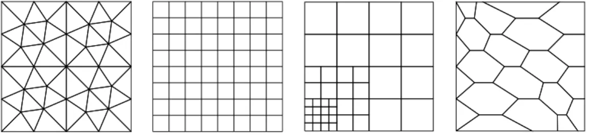
with p P t2, 3, 4u and source term inferred from u (cf. (21) for the expression of a in this case). We consider the matching triangular, Cartesian, locally refined, and (predominantly) hexagonal mesh families depicted in Figure 1 and polynomial degrees ranging from 0 to 3. The three former mesh families are taken from the FVCA5 benchmark [31], whereas the latter is taken from [19]. The local refinement in the third mesh family has no specific meaning for the problem considered here: its purpose is to demonstrate the seamless treatment of nonconforming interfaces.

Figure 1: Matching triangular, Cartesian, locally refined and hexagonal mesh families used in the numerical examples of Section 3.5.

We report in Figure 2 the error }Ikhu ´ uh}1,p,h versus the meshsize h. From the leftmost column,

we see that the error estimates are sharp for p “ 2, which confirms the results of [17] (a known superconvergence phenomenon is observed on the Cartesian mesh for k “ 0). For p “ 3, 4, better orders of convergence than the asymptotic ones (cf. Remark 8) are observed in most of the cases. One possible explanation is that the lowest-order terms in the right-hand side of (36) are not yet dominant for the specific problem data and mesh at hand. Another possibility is that compensations occur among lowest-order terms that are separately estimated in the proof of Theorem 7. For k “ 3 and p “ 3, the observed orders of convergence in the last refinement steps are inferior to the predicted value for smooth solutions, which can likely be ascribed to the violation of the regularity assumption on ap¨, ∇uq (cf. Theorem 7), due to the lack of smoothness of a for that p.

A

Inequalities involving the Leray–Lions operator

This section collects inequalities involving the Leray–Lions operator adapted from [23]. Lemma 15. Assume (20c), (20e), and p ď 2. Then, for a.e. x P Ω and all pξ, ηq P Rd

ˆ Rd, |apx, ξq ´ apx, ηq| ď p2γa` 2p´1βa` βaq|ξ ´ η|p´1. (66)

Proof. Let r ą 0. If |ξ| ě r and |η| ě r then, using (20e) and p ´ 2 ď 0, we have

|apx, ξq ´ apx, ηq| ď γa|ξ ´ η|p|ξ|p´2` |η|p´2q ď 2γarp´2|ξ ´ η|. (67)

Otherwise, assume for example that |η| ă r. Then |ξ| ď |ξ ´ η| ` r and thus, owing to (20c), |apx, ξq ´ apx, ηq| ď |apx, ξq ´ apx, 0q| ` |apx, 0q ´ apx, ηq|

ď βap|ξ|p´1` |η|p´1q

ď βap|ξ ´ η| ` rqp´1` βarp´1. (68)

Combining (67) and (68) shows that, in either case,

|apx, ξq ´ apx, ηq| ď 2γarp´2|ξ ´ η| ` βap|ξ ´ η| ` rqp´1` βarp´1.

Taking r “ |ξ ´ η| concludes the proof of (66).

Lemma 16. Under Assumption (20f) we have, for a.e. x P Ω and all pξ, ηq P Rd

ˆ Rd, • If p ă 2, |ξ ´ η|pď ζ´ p 2 a 2pp´1q 2´p 2 ´ rapx, ξq ´ apx, ηqs ¨ rξ ´ ηs ¯p₂´ |ξ|p` |η|p ¯2´p₂ ; (69)

k “ 0 k “ 1 k “ 2 k “ 3 10´2.5 ₁₀´2 ₁₀´1.5 10´8 10´6 10´4 10´2 1 1 1 2 1 3 1 4 (a) Triangular, p “ 2 10´2.5 ₁₀´2 ₁₀´1.5 10´5 10´4 10´3 10´2 10´1 1 1/2 1 1 1 3/2 1 2 (b) Triangular, p “ 3 10´2.5 ₁₀´2 ₁₀´1.5 10´5 10´4 10´3 10´2 10´1 1 1/3 1 2/3 1 1 1 4/3 (c) Triangular, p “ 4 10´2.5 ₁₀´2 ₁₀´1.5 10´8 10´7 10´6 10´5 10´4 10´3 10´2 10´1 1 1 1 2 1 3 1 4 (d) Cartesian, p “ 2 10´2.5 ₁₀´2 ₁₀´1.5 10´4 10´3 10´2 10´1 1 1/2 1 1 1 3/2 1 2 (e) Cartesian, p “ 3 10´2.5 ₁₀´2 ₁₀´1.5 10´3 10´2 10´1 1 1/3 1 2/3 1 1 1 4/3 (f) Cartesian, p “ 4 10´1.5 ₁₀´1 ₁₀´0.5 10´8 10´7 10´6 10´5 10´4 10´3 10´2 10´1 1 1 1 2 1 3 1 4 (g) Loc. ref., p “ 2 10´1.5 ₁₀´1 ₁₀´0.5 10´4 10´3 10´2 10´1 1 1/2 1 1 1 3/2 1 2 (h) Loc. ref., p “ 3 10´1.5 ₁₀´1 ₁₀´0.5 10´3 10´2 10´1 1 1/3 1 2/3 1 1 1 4/3

(i) Loc. ref., p “ 4

10´2.4₁₀´2.2₁₀´2₁₀´1.8₁₀´1.6₁₀´1.4₁₀´1.2 10´7 10´6 10´5 10´4 10´3 10´2 10´1 1 1 1 2 1 3 1 4 (j) Hexagonal, p “ 2 10´2.4₁₀´2.2₁₀´2₁₀´1.8₁₀´1.6₁₀´1.4₁₀´1.2 10´4 10´3 10´2 10´1 1 1/2 1 1 1 3/2 1 2 (k) Hexagonal, p “ 3 10´2.4₁₀´2.2₁₀´2₁₀´1.8₁₀´1.6₁₀´1.4₁₀´1.2 10´3 10´2 10´1 1 1/3 1 2/3 1 1 1 4/3 (l) Hexagonal, p “ 4 Figure 2: }Ikhu ´ uh}1,p,hversus h for the mesh families of Figure 1. The slopes represent the orders

• If p ě 2,

|ξ ´ η|pď ζ_a´1rapx, ξq ´ apx, ηqs ¨ rξ ´ ηs. (70)

Proof. Estimate (69) is obtained by raising (20f) to the power p{2 and using p|ξ| ` |η|qp ď 2p´1p|ξ|p` |η|pq. To prove (70), we simply write |ξ ´ η|pď |ξ ´ η|2p|ξ| ` |η|qp´2.

Remark 17. The (real-valued) mapping a : t ÞÑ |t|p´2_{t corresponds to the p-Laplace operator in}

dimension 1, and it therefore satisfies (20f). Hence, by Lemma 16, If p ă 2: |t ´ r|pď C`“|t|p´2t ´ |r|p´2r‰rt ´ rs˘ p 2 p|t|p` |r|pq 2´p p _{, (71)} If p ě 2: |t ´ r|pď C“|t|p´2t ´ |r|p´2r‰rt ´ rs, (72) where C depends only on p.

References

[1] B. Andreianov, F. Boyer, and F. Hubert. On the finite-volume approximation of regular solutions of the p-Laplacian. IMA J. Numer. Anal., 26:472–502, 2006.

[2] P. F. Antonietti, N. Bigoni, and M. Verani. Mimetic finite difference approximation of quasilinear elliptic problems. Calcolo, 52:45–67, 2014.

[3] B. Ayuso de Dios, K. Lipnikov, and G. Manzini. The nonconforming virtual element method. ESAIM: Math. Model Numer. Anal. (M2AN), 50(3):879–904, 2016.

[4] J. W. Barrett and W. B. Liu. Quasi-norm error bounds for the finite element approximation of a non-Newtonian flow. Numer. Math., 68(4):437–456, 1994.

[5] L. Beir˜ao da Veiga, F. Brezzi, A. Cangiani, G. Manzini, L. D. Marini, and A. Russo. Basic principles of virtual element methods. Math. Models Methods Appl. Sci. (M3AS), 199(23):199–214, 2013.

[6] L. Beir˜ao da Veiga, K. Lipnikov, and G. Manzini. The Mimetic Finite Difference Method for Elliptic Problems, volume 11 of Modeling, Simulation and Applications. Springer, 2014.

[7] S. C. Brenner and L. R. Scott. The mathematical theory of finite element methods, volume 15 of Texts in Applied Mathematics. Springer, New York, third edition, 2008.

[8] F. Brezzi, K. Lipnikov, and M. Shashkov. Convergence of the mimetic finite difference method for diffusion problems on polyhedral meshes. SIAM J. Numer. Anal., 43(5):1872–1896, 2005.

[9] F. Chave, D. A. Di Pietro, F. Marche, and F. Pigeonneau. A Hybrid High-Order method for the Cahn–Hilliard problem in mixed form. SIAM J. Numer. Anal., 2016. Accepted for publication. Preprint arXiv:1509.07384 [math.NA].

[10] B. Cockburn, D. A. Di Pietro, and A. Ern. Bridging the Hybrid High-Order and Hybridizable Discontinuous Galerkin methods. ESAIM: Math. Model. Numer. Anal. (M2AN), 50(3):635–650, 2016.

[11] B. Cockburn, J. Gopalakrishnan, and F.-J. Sayas. A projection-based error analysis of HDG methods. Math. Comp., 79:1351–1367, 2010.

[12] B. Cockburn, W. Qiu, and K. Shi. Conditions for superconvergence of HDG methods for second-order elliptic problems. Math. Comp., 81:1327–1353, 2012.

[13] D. A. Di Pietro and J. Droniou. A Hybrid High-Order method for Leray–Lions elliptic equations on general meshes. Math. Comp., 2016. Accepted for publication. Preprint arXiv:1508.01918 [math.NA].

[14] D. A. Di Pietro, J. Droniou, and A. Ern. A discontinuous-skeletal method for advection–diffusion–reaction on general meshes. SIAM J. Numer. Anal., 53(5):2135–2157, 2015.

[15] D. A. Di Pietro and A. Ern. A hybrid high-order locking-free method for linear elasticity on general meshes. Comput. Meth. Appl. Mech. Engrg., 283:1–21, 2015.

[16] D. A. Di Pietro and A. Ern. Arbitrary-order mixed methods for heterogeneous anisotropic diffusion on general meshes. IMA J. Numer. Anal., 2016. Published online. DOI 10.1093/imanum/drw003.

[17] D. A. Di Pietro, A. Ern, and S. Lemaire. An arbitrary-order and compact-stencil discretization of diffusion on general meshes based on local reconstruction operators. Comput. Meth. Appl. Math., 14(4):461–472, 2014. [18] D. A. Di Pietro, A. Ern, A. Linke, and F. Schieweck. A discontinuous skeletal method for the

viscosity-dependent Stokes problem. Comput. Meth. Appl. Mech. Engrg., 306:175–195, 2016.

[19] D. A. Di Pietro and S. Lemaire. An extension of the Crouzeix–Raviart space to general meshes with application to quasi-incompressible linear elasticity and Stokes flow. Math. Comp., 84(291):1–31, 2015.

[20] J. I. Diaz and F. de Thelin. On a nonlinear parabolic problem arising in some models related to turbulent flows. SIAM J. Math. Anal., 25(4):1085–1111, 1994.

[21] J. Droniou. Finite volume schemes for fully non-linear elliptic equations in divergence form. ESAIM: Math. Model Numer. Anal. (M2AN), 40:1069–1100, 2006.

[22] J. Droniou and R. Eymard. A mixed finite volume scheme for anisotropic diffusion problems on any grid. Numer. Math., 105:35–71, 2006.

[23] J. Droniou, R. Eymard, T. Gallou¨et, C. Guichard, and R. Herbin. Gradient schemes for elliptic and parabolic problems. 2016. In preparation.

[24] J. Droniou, R. Eymard, T. Gallou¨et, and R. Herbin. A unified approach to mimetic finite difference, hybrid finite volume and mixed finite volume methods. Math. Models Methods Appl. Sci. (M3AS), 20(2):1–31, 2010. [25] J. Droniou, R. Eymard, T. Gallouet, and R. Herbin. Gradient schemes: a generic framework for the discreti-sation of linear, nonlinear and nonlocal elliptic and parabolic equations. Math. Models Methods Appl. Sci. (M3AS), 23(13):2395–2432, 2013.

[26] T. Dupont and R. Scott. Polynomial approximation of functions in Sobolev spaces. Math. Comp., 34(150):441– 463, 1980.

[27] R. Eymard, T. Gallou¨et, and R. Herbin. Discretization of heterogeneous and anisotropic diffusion problems on general nonconforming meshes. SUSHI: a scheme using stabilization and hybrid interfaces. IMA J. Numer. Anal., 30(4):1009–1043, 2010.

[28] R. Eymard, C. Guichard, and R. Herbin. Small-stencil 3D schemes for diffusive flows in porous media. ESAIM Math. Model. Numer. Anal., 46(2):265–290, 2012.

[29] R. Glowinski. Numerical methods for nonlinear variational problems. Springer Series in Computational Physics. Springer-Verlag, New York, 1984.

[30] R. Glowinski and J. Rappaz. Approximation of a nonlinear elliptic problem arising in a non-Newtonian fluid flow model in glaciology. ESAIM: Math. Model Numer. Anal. (M2AN), 37(1):175–186, 2003.

[31] R. Herbin and F. Hubert. Benchmark on discretization schemes for anisotropic diffusion problems on general grids. In R. Eymard and J.-M. H´erard, editors, Finite Volumes for Complex Applications V, pages 659–692. John Wiley & Sons, 2008.

[32] Y. Kuznetsov, K. Lipnikov, and M. Shashkov. Mimetic finite difference method on polygonal meshes for diffusion-type problems. Comput. Geosci., 8:301–324, 2004.

[33] W. Liu and N. Yan. Quasi-norm a priori and a posteriori error estimates for the nonconforming approximation of p-Laplacian. Numer. Math., 89:341–378, 2001.