3D Mesh Animation Compression based on adaptive spatio-temporal segmentation

(1)

HAL Id: hal-03078907

https://hal.archives-ouvertes.fr/hal-03078907

Submitted on 16 Dec 2020

HAL is a multi-disciplinary open access

archive for the deposit and dissemination of

sci-entific research documents, whether they are

pub-lished or not. The documents may come from

teaching and research institutions in France or

abroad, or from public or private research centers.

L’archive ouverte pluridisciplinaire HAL, est

destinée au dépôt et à la diffusion de documents

scientifiques de niveau recherche, publiés ou non,

émanant des établissements d’enseignement et de

recherche français ou étrangers, des laboratoires

publics ou privés.

3D Mesh Animation Compression based on adaptive

spatio-temporal segmentation

Guoliang Luo, Zhigang Deng, Xiaogag Jin, Xin Zhao, Wei Zeng, Wenqiang

Xie, Hyewon Seo

To cite this version:

Guoliang Luo, Zhigang Deng, Xiaogag Jin, Xin Zhao, Wei Zeng, et al.. 3D Mesh Animation

Compres-sion based on adaptive spatio-temporal segmentation. ACM SIGGRAPH Symposium on Interactive

3D Graphics and Games (I3D 2019), May 2019, Montréal, Canada. pp.10, �10.1145/3306131.3317017�.

�hal-03078907�

(2)

3D Mesh Animation Compression based on Adaptive

Spatio-temporal Segmentation

Guoliang Luo

∗

East China Jiaotong University Nanchang, China luoguoliang@ecjtu.edu.cn

Zhigang Deng

∗ University of Houston Texas, USA zdeng4@uh.edu

Xiaogang Jin

Zhejiang University Hangzhou, China jin@cad.zju.edu.cn

Xin Zhao

East China Jiaotong University Nanchang, China

Wei Zeng

Jiangxi Normal University Nanchang, China

Wenqiang Xie

Jiangxi Normal University Nanchang, China

Hyewon Seo

Univerisity of Strasbourg Strasbourg, France

ABSTRACT

With the recent advances of data acquisition techniques, the com-pression of various 3D mesh animation data has become an im-portant topic in computer graphics community. In this paper, we present a new spatio-temporal segmentation-based approach for the compression of 3D mesh animations. Given an input mesh se-quence, we first compute an initial temporal cut to obtain a small subsequence by detecting the temporal boundary of dynamic behav-ior. Then, we apply a two-stage vertex clustering on the resulting subsequence to classify the vertices into groups with optimal intra-affinities. After that, we design a temporal segmentation step based on the variations of the principle components within each vertex group prior to performing a PCA-based compression. Our approach can adaptively determine the temporal and spatial segmentation boundaries in order to exploit both temporal and spatial redun-dancies. We have conducted many experiments on different types of 3D mesh animations with various segmentation configurations. Our comparative studies show the competitive performance of our approach for the compression of 3D mesh animations.

CCS CONCEPTS

• Computing methodologies → Computer graphics; Anima-tion;

KEYWORDS

3D mesh animation, compression, adaptive spatio-temporal seg-mentation

∗_{Correspondence authors, both authors contributed equally to the paper.}

Permission to make digital or hard copies of all or part of this work for personal or classroom use is granted without fee provided that copies are not made or distributed for profit or commercial advantage and that copies bear this notice and the full citation on the first page. Copyrights for components of this work owned by others than ACM must be honored. Abstracting with credit is permitted. To copy otherwise, or republish, to post on servers or to redistribute to lists, requires prior specific permission and/or a fee. Request permissions from permissions@acm.org.

ACM Reference Format:

Guoliang Luo, Zhigang Deng, Xiaogang Jin, Xin Zhao, Wei Zeng, Wenqiang Xie, and Hyewon Seo. 2019. 3D Mesh Animation Compression based on Adaptive Spatio-temporal Segmentation. In Symposium on Interactive 3D Graphics and Games (I3D ’19), May 21–23, 2019, Montreal, QC, Canada. ACM, New York, NY, USA, 10 pages. https://doi.org/10.1145/3306131.3317017

1 INTRODUCTION

The key information of a 3D mesh animation is its dynamic behav-ior, which drives the deformations of different mesh surface areas. As reported in existing literature, we can achieve a better perfor-mance on the compression of 3D mesh animations with repetitive motions or rigid mesh segments, which contain significant redun-dancies either temporally or spatially [Lalos et al. 2017; Stefanoski and Ostermann 2010; Váša et al. 2014]. Therefore, it is important to exploit the dynamic behaviors based on both spatial and tempo-ral segmentations within a 3D mesh animation for effective data compression. However, due to the high complexity and the large data size, it remains a challenge to jointly explore the spatial and temporal segmentations to further improve the performance of 3D mesh animation compression.

In this paper, we propose an adaptive spatio-temporal segmen-tation based model for the compression of 3D mesh animations. Specifically, we first introduce a temporal segmentation scheme that explores the temporal redundancy by automatically determin-ing the optimal temporal boundaries. Then, we also introduce a novel two-stages vertex clustering approach to explore the spatial redundancy by automatically determining the number of the ver-tex groups with optimal intra-affinities. As an application of the above adaptive spatio-temporal segmentation model, we develop a full scheme for the compression of 3D mesh animations (Figure 1). Through many experiments, we show the effectiveness and effi-ciency of our approach, compared to the state of the art 3D mesh animation compression algorithms.

The contributions of this work can be summarized as follows: • an adaptive spatio-temporal segmentation approach which

explores both the spatial and temporal redundancies for 3D mesh animations; and

(3)

• a compression model for 3D mesh animations by coupling the novel adaptive spatio-temporal segmentation and the compression of 3D mesh animations.

The remainder of this paper is organized as follows. We first review previous and related works on the compression of 3D mesh animations in Section 2. In Section 3, we briefly give the overview of our compression scheme. Then, we present the details of our spatio-temporal segmentation model and its application to the com-pression of 3D mesh animations in Section 4. The experimental results by our model are shown in Section 5. Finally, we conclude this work in Section 6.

2 RELATED WORK

The compression of 3D mesh animation data has been a persistent research topic in the past several decades [Maglo et al. 2015].Among the existing methods, a large portion of the methods take a matrix form of the 3D mesh animation, on which many of classical data compression methods and algorithms can be applied, including Principal Component Analysis (PCA) [Alexa and Müller 2000; Hou et al. 2017; Liu et al. 2012], linear prediction encoders [Karni and Gotsman 2004; Stefanoski et al. 2007; Stefanoski and Ostermann 2010; Yang et al. 2002], wavelet decomposition [Guskov and Kho-dakovsky 2004; Payan and Antonini 2007], and the Moving Picture Experts Group (MPEG) framework [Mamou et al. 2008]. PCA is a classical method that can decompose a large matrix as the product of two much smaller matrices, with minimal information loss. Fol-lowing the work of [Alexa and Müller 2000], Lee et al. [2007] apply PCA to 3D mesh animation data after removing its rigid transfor-mations. Later, researchers have used the linear prediction theory to further encode the resulting coefficients from PCA [Karni and Gotsman 2004; Vasa and Skala 2009; Váša and Brunnett 2013]. Simi-larly, researchers have proposed a Laplacian-based spatio-temporal predictor [Váša et al. 2014] or curvature-and-torsion based analysis [Yang et al. 2018] to encode the vertex trajectories for dynamic meshes. However, they assume an entire sequence as the given in-put, and do not explicitly exploit the dynamic behaviors enclosed in the input animation. The key information of a 3D mesh animation is its enclosed dynamic behavior; therefore, it is important to exploit the dynamic behavior coherence in 3D mesh animations for effec-tive compression, using either spatial segmentation or temporal segmentation methods.

Spatial segmentation based compression: The key of the spatial segmentation of a 3D mesh animation is to understand its semantic behaviors. Many previous methods have been proposed to compute the spatial segmentations for 3D mesh animations, which can gen-erate different spatial segmentation schemes for animations with different motions [A Vasilakis and Fudos 2014; de Aguiar et al. 2008; James and Twigg 2005; Kavan et al. 2010; Le and Deng 2014; Lee et al. 2006; Wuhrer and Brunton 2010]. Hijiri et al. [2000] separately compress the vertices of each object with the same movements to obtain an overall optimal compression rate. In order to adapt spatial segmentation for compression, Sattler et al. [2005] proposed an iterative clustered PCA method to group the vertex trajecto-ries that share similar Principal Component (PC) coefficients and then further compress each cluster separately. Its main limitation is its heavy computational cost. Similarly, Ramanathan et al. [2008]

compute the optimal vertex clustering for the optimal compression ratio. However, all the above methods assume the entire animation has been given at the beginning.

Temporal segmentation based compression: The objective of tem-poral segmentation is mainly to chop a 3D mesh animation into sub-sequences, each of which represents a different dynamic behav-ior. Temporal segmentation has been exploited for the compression of motion capture data [Gong et al. 2012; Gu et al. 2009; Sattler et al. 2005; Zhu et al. 2012], but the efficiencies of these methods for 3D mesh animation compression may be significantly decreased since 3D mesh surfaces typically have much more denser vertices and additional topology than motion capture data [Luo et al. 2017]. Given a mesh sequence, Luo et al. [2013] group the meshes with similar poses and apply PCA to compress each group to achieve the optimal compression ratio. Recently, Lalo et al. [2017] proposed an adaptive Singular Value Decomposition (SVD) coefficient method for 3D mesh animation compression. They first divide a mesh se-quence into temporal blocks of the same length and treat the first block with SVD. Then, the following blocks are treated with the adaptive bases from the previous block without solving the full SVD decomposition for each block, which reduces the compute time.

In summary, spatial and temporal segmentations can help to re-veal the spatial and temporal redundancies within 3D mesh anima-tions, which benefits for the development of effective compression algorithms. The new compression scheme for 3D mesh animations, presented in this work alternately exploits both spatial and temporal redundancies.

3 SCHEME OVERVIEW

In general 3D mesh animations mainly have two different forms, namely, time-varying meshes and deforming meshes. A time-varying mesh may have different numbers of vertices and different topologi-cal connectivities at different frames, whereas a deforming mesh has a fixed topology across frames. Note that we can always compute the inter-frame vertex correspondences to convert a time-varying mesh into a deforming mesh [Tevs et al. 2012]. For the sake of simplicity, we focus on the deforming mesh data in this work.

Then, we define the trigger conditions for the two important steps in our method. (1) Initial Temporal Cut: given the maximal length γinitif any dynamic behavior has been detected in the mesh sequence (with no more than γinitframes) (see Section 4.1), and (2) Actual Temporal Segmentation: given the maximal length γact if any dynamic behavior has been detected in any of the vertex groups (see Section 4.2 and 4.3).

We briefly describe the pipeline of our segmentation scheme as follows. The algorithmic description is also shown in Figure 1.

(1) We first conduct an initial temporal cut to produce a sub-sequence S with the maximal possible length of γinit, see Section 4.1.

(2) If no distinct behavior can be detected in S, i.e., the boundary frame b= γinit, the subsequence S will be directly sent to the compressor (the case (I) in Section 4.5), see Section 4.4. (3) Otherwise (i.e., distinct behaviors are detected in S), we

(4)

3D Mesh Animation Compression based on Adaptive Spatio-temporal Segmentation I3D ’19, May 21–23, 2019, Montreal, QC, Canada

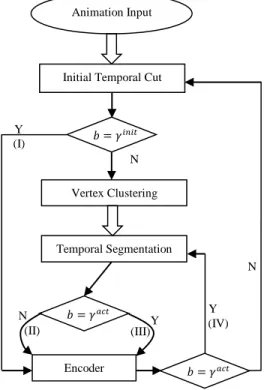
Initial Temporal Cut Animation Input Vertex Clustering Temporal Segmentation Encoder N _Y N Y Y N 𝑏 = 𝛾𝑖𝑛𝑖𝑡 𝑏 = 𝛾𝑎𝑐𝑡 𝑏 = 𝛾𝑎𝑐𝑡 (IV) (III) (II) (I)

Figure 1: Pipeline overview of our spatio-temporal segmen-tation scheme for compression. (I, II, III, and IV) are the 4 types of the segmented animation blocks, which are ex-plained in Section 4.5. Note that b denotes the length of an initial/actual temporal segmentation, γinit and γact are the maximal possible lengths for the Initial Temporal Cut and the Temporal Segmentation (short for the Actual Temporal Segmentation), respectively.

(4) Then, we continue to compute the temporal segmentation of each vertex group (spatial segment) within next γactframes, by analyzing the dynamic behaviors, see Section 4.3. (5) If we have detected distinct dynamic behaviors of any vertex

group before γact is reached, the vertex trajectories of each group up to the detected boundary frame are sent to the compressor, separately. See Section 4.4. After the compres-sion, we repeat the process from the step 1 (the case (II) in Section 4.5).

(6) Otherwise (i.e., we have not detected a temporal segmen-tation before reaching γact), we also send the data of each vertex cluster to the compressor, separately (the case (III) in Section 4.5). See Section 4.4. Afterwards, we reuse the previously obtained vertex clustering and continue the anal-ysis of the temporal segmentation in the remaining mesh frames. That is, we repeat the process from the step 4 for the remaining mesh frames (The case (IV) in Section 4.5).

4 SPATIO-TEMPORAL SEGMENTATION FOR

COMPRESSION

We first describe our spatio-temporal segmentation model that consists of the initial temporal cut (Section 4.1), vertex clustering (Section 4.2), and temporal segmentation (Section 4.3). Then, we apply the spatio-temporal segmentation model for the compression of 3D mesh animations in Section 4.4. Finally, we discuss different scenarios while processing a continuous mesh sequence as the input in Section 4.5.

4.1 Initial Temporal Cut

Let us denote a mesh animation as ({Vf_i}, E), where E represents the connectivities among the vertices, and Vf_i = (x_if,yf_i, zf_i) represents the 3D coordinates of the i-th vertex (i= 1, . . . ,V ) at the f -th frame (f = 1, . . . , F). Here V is the total number of vertices, and F is the total number of frames in the animation sequence.

Given a mesh sequence, the objective of the initial temporal cut is to determine a boundary frame V|τ |, so that the dynamic behavior in [V1, V|τ |] is distinctive from that in [V|τ |+1, Vγi ni t]. To this end, we can formulate the initial temporal cut as the following optimization problem:

min

b ∈[1,γi ni t]I ([V

1_{, V}b_{], [V}b+1_{, V}γi ni t

]), (1) where b is a to-be-solved frame index and I (·, ·) computes the affinity between two mesh subsequences.

Available techniques for computing I (·, ·) can be classified into two categories: 1) front-to-end, uni-directional boundary candidate search, and 2) bi-directional boundary candidate search. Between them, the bi-direction search method is more robust on detecting the temporal cut between two successive dynamic behaviors [Barbič et al. 2004; Gong et al. 2012]. Inspired by the kernelized Canonical Correlation Analysis (kCCA) approach [Hofmann et al. 2008; Smola et al. 2007], and its successful application to semantic temporal cut for motion capture data [Gong et al. 2012], we formulate the initial temporal cut to a Maximum-Mean Discrepancy problem as follows:

min bi∈[1,γi ni t−ϵ]− © « 1 |T1|2 Í|T1| i, j K(vbi:bi+ϵ, vbj:bj+ϵ) −_|T11_{| |T2}_|Í|T1| i Í|jT2|K(vbi:bi+ϵ, vbj:bj+ϵ) + 1 |T2|2 Í|T2| i, j K(vbi:bi+ϵ, vbj:bj+ϵ) ª ® ® ® ¬ , (2)

whereT1is the subsequence [V1, . . . , Vbi] andT2is the subsequence

[Vbi+1, . . . , Vγi ni t−ϵ], and ϵ is a pre-defined parameter to ensure smooth kernels.

The kernel function in Eq. 2 is defined as follows:

K(vbi:bi+ϵ, vbj:bj+ϵ)= exp(−λ∥vbi:bi+ϵ− vbj:bj+ϵ∥2), (3) where λ is the kernel parameter for K(·) [Van Vaerenbergh 2010]. Due to the symmetric property of the kCCA, i.e., K(A, B)= K(B, A), we obtain a symmetric kCCA matrix for the animation block.

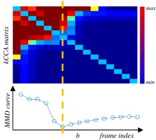
Finally, we can obtain a boundary frame V|τ | for the initial temporal cut by solving the objective function in (Eq. 2). Note that |τ |= b + ϵ due to the usage of a smoothing window. Meanwhile, we denote the detected initial temporal cut as τ . Figure 2 shows one of the initial temporal cuts of the ‘March’ data, with γinit = 20 and ϵ= 5.

(5)

max frame index MM D c u rve b kCC A ma trix min

Figure 2: An example of the initial temporal segmentation of the ‘March’ data, with the pairwise frame based kCCA ma-trix (Eq. 3) in the top panel and the MMN curve (Eq. 2) in the bottom panel. b is the detected boundary frame. The color-bar indicates the small (blue) and large (red) kernels.

The complexity of the above bi-directional search for the initial temporal cut is O(|γinit|2), which is less efficient than the uni-directional methods with O(|γinit|). However, in our context, we compute the initial temporal cut within a short mesh sequence [1, γinit], which is a small cost on the computation and thus will not cause notable delay to the overall compression framework. The settings of γinitfor different experimental data are presented in Table 1.

4.2 Vertex Clustering

In this section, we describe a vertex clustering (spatial segmen-tation) algorithm based on a two-stages, bottom-up hierarchical clustering algorithm to obtain optimal spatial affinities within seg-ments.

4.2.1 Initial Vertex Clustering. After the initial temporal cut, τ is obtained; we then compute the vertex clustering based on the dy-namic behaviors of different vertices. The pipeline of our approach is shown in Figure 3 (I,II,III).

In this initial vertex clustering stage, we first segment a dynamic mesh based on rigidity with the following steps.

(1) Compute the MEC for all edge pairs. Similar to [Lee et al. 2006; Wuhrer and Brunton 2010], we compute the Maximal Edge-length Change (MEC) within |τ | frames for each vertex pair, see Figure 3(I).

(2) Binary labeling of vertices. We fit the MEC of all the edges as an exponential distribution epd, see the top of Figure 3(I). Then, with the aid of the inverse cumulative distribution function of epd, we can determine a user-specified percent of the edges as the rigid edges (ρ= 20% in our experiments). Thus, the vertices that are connected to the rigid edges are

( Ⅰ ) ( Ⅱ ) ( Ⅲ ) ( Ⅳ ) ‘deformed’

‘rigid’

Figure 3: Pipeline of the vertex clustering within an initial temporal cut of the ‘March’ data: (I) Maximal Edge-length Change (MEC) for all the edge pairs and their distributions, (II) binary labeling of vertices, (III) the rigid clusters resulted from the initial vertex clustering, and (IV) the rigid cluster grouping results.

called the rigid vertices, and the remaining vertices are called the deformed vertices in this work, see Figure 3(II). (3) Identify the rigid regions. Based on the above binary labeling

results, we merge the topologically connected rigid vertices into rigid regions, which become initial rigid vertex clusters. We also compute the center of each cluster as the average vertex trajectory of each cluster.

(4) Rigid clusters growing. Starting with the above rigid clusters, we repeatedly merge the connected neighboring deformed vertices into the rigid cluster with the most similar trajecto-ries, and update the center of the corresponding rigid cluster. The initial vertex clustering is completed till every deformed vertex has been merged into a rigid cluster δi(i= 1, . . . ,k, k is the total number of the clusters), see Figure 3(III).

4.2.2 Rigid Cluster Grouping. In the second-stage vertex clustering, we further classify the rigid clusters to ω groups with high internal affinities. In [Sattler et al. 2005], Sattler et al. proposed an iterative clustered PCA based model for animation sequence compression. Inspired by this work, we design the second-stage vertex clustering by iteratively classifying and assigning each rigid cluster to the group with the minimal reconstruction error until the grouping remains unchanged. Since the iterative clustered-PCA is performed on the initial vertex cluster, it works very efficiently, unlike the case in [Sattler et al. 2005].

The reconstruction error of a rigid cluster δjis defined as follows: ∥δj− eδj∥2= ∥δj− (C[j]+ bδj)∥2, (4) where eδj is the reconstructed cluster using PCA, C[j] is the center of each group (j = 1, . . . , ω), and bδj is the reconstruction using the PCA components (see Eq. 6). Note that we have C[j] in Eq. 4, because PCA contains the centering (mean subtraction) of the input data for the covariance matrix calculation.

Figure 3 illustrates the process of the rigid cluster grouping with the ‘March’ data. As an example result in Figure 3(IV), the relatively less moved rigid clusters, ‘head’, ‘chest’ and ‘right-arm’, are classi-fied into the same group. Note that we obtain large vertex groups

(6)

because the input mesh are smooth on the surface (see Table 1), un-like the motion Capture data containing sparse vertex trajectories that may lead to small groups. Moreover, the computational cost for the initial vertex clustering presented above is relatively small because both the number of clusters k and the number of groups ω are small.

4.3 Temporal Segmentation

After obtaining a set of the spatio-temporal segments L(δ )j(j = 1, . . . , ω) for the initial temporal cut τ , we further introduce a tem-poral segmentation step as follows:

• For each vertex group, we stop observing the number of PCs once it is changed within the current sliding window. In this way, we can obtain a Num-of-PCs curve for each vertex group, see the bottom of Figure 4.

• To this end, similar to [Karni and Gotsman 2004], the tempo-ral segmentation boundary is determined as the first frame where any Num-of-PCs curve has changes, see the bottom-right of Figure 4.

The complexity of the temporal segmentation is O(ωγact), where γactdenotes the maximal length of temporal segments. Note that the computational cost of the PCA decomposition increases exponen-tially with the input data size. In order to balance the computational cost and the effectiveness of PCA, we set an adaptive γactfor each of the input data, see Table 1.

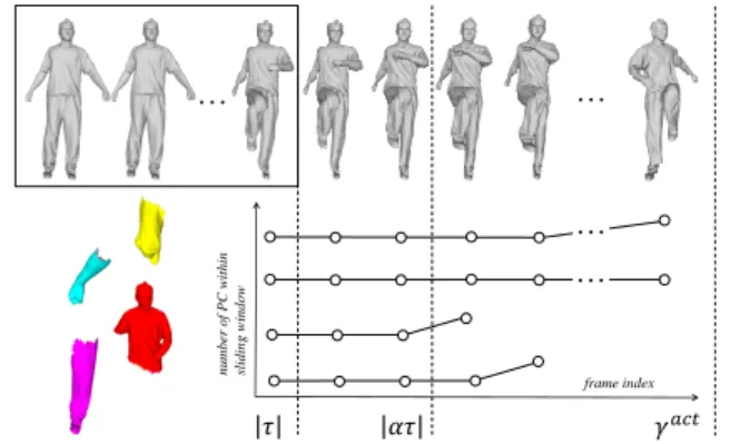
… … … 𝛾𝑎𝑐𝑡 𝜏 … 𝛼𝜏 frame index num ber of PC within sliding windo w

Figure 4: Illustration of the temporal segmentation. The top row shows a sampled mesh sequence, with a bounding box as a sliding window. The size of the window is dynamically determined as the length of the initial temporal cut, i.e., |τ |. The bottom-left shows the vertex grouping of the initial tem-poral segment, and the bottom-right contains the change of the number of PCs for each vertex group in the sliding win-dow. γact is the maximal possible delay, and |ατ | is the de-tected temporal segmentation boundary.

Parallel computing. The temporal segmentation presented above is designed for each vertex group (spatio-temporal segment), and the vertex groups are independent of each other. Thus, we can implement the temporal segmentation for each vertex group in parallel. The computational time statistics in Table 1 show the efficiency improvement through parallelization.

4.4 Compression

After the above spatio-temporal segmentation, we apply PCA to compress each segment with a pre-defined threshold on the infor-mation persistence rate, µ ∈ [0 1], which is used to determine the number of PCs to retain after the PCA decomposition, i.e.,

k Õ i (σi)/ |n | Õ i (σi) ≥ µ, (5) where k ≤ n, and {σi}(i = 1, . . . ,n) are the eigen-values of the data block in a descending order. Therefore, we can control the compression quality by manipulating the value of µ. In specific, by increasing µ, we have less information loss but more storage costs after compression; and vice-versa.

• Encoder. For a spatio-temporal segment L(δ )i_j, i.e., the j-th spatial segment within the i-th actual temporal segment ατi, we denote its compression as follows:

Vατi_{L(δ )}i j

PCA

≈ Ai_j× Bi_j, (6) where Ai_j is the score matrix of dimensions 3|V_{L(δ )}i

j| × k i j, Bij is

the coefficient matrix of dimensions ki_j × |ατi|, and bX denotes a centered matrix of X by subtracting the mean vectors X, i.e.,

b

X= X − X. (7) • Decoder. With the score matrix and the coefficient matrix, we can approximate each of the spatio-temporal segments using Eq. 6 and Eq. 7. Then, we can reconstruct the original animation by concatenating the spatio-temporal segments in order.

4.5 Sequential Processing

As discussed in Section 3, our spatio-temporal segmentation scheme generates four possible animation blocks that are further sent to the encoder for compression (see Figure 1), which leads to four types of sequential processing to the successive mesh sequence:

(I) |τ |= γinit. This indicates none of distinct behaviors has been detected at the initial temporal cut step (Section 4.1). In this case, the animation block [V1, Vγi ni t] will be directly sent to the encoder. Moreover, we need to re-compute a spatio-temporal segmentation for the successive mesh sequence.

(II) |τ | < γinitand |ατ | < γact. This indicates the vertex clus-tering has been conducted and a temporal segmentation boundary has been detected at V|ατ |. In this case, each vertex group of the an-imation block will be sent to the encoder, separately. Moreover, we will re-compute a spatio-temporal segmentation for the successive mesh sequence.

(III) |τ | < γinitand |ατ |= γact. This indicates the vertex cluster-ing has been conducted and a temporal segmentation boundary has not been detected within the range [V1, Vγac t]. In this case, each vertex group of the animation block will be sent to the encoder, separately. Moreover, we will only need to re-compute the temporal segmentation for the successive mesh sequence.

(IV) Otherwise, we can directly reuse the existing (previous) vertex grouping results, compute the temporal segmentation, and then perform the PCA-based compression for each vertex group. If the new boundary |ατ | < γact, we will need to re-compute a

(7)

Table 1: The results and performances by our model with different configurations of parameters: ϵ and γinit for the Initial Temporal Segmentation (Section 4.1), γact for the Actual Temporal Segmentation (Section 4.3) and ω for the vertex clustering (Section 4.2). s and spare the timings in seconds (unit) of the single-thread and paralleled implementations, respectively, with the last column showing the percentage of the time savings for each data.

Animations Vertex Frame Parameters Rate KGError Timing

V F ϵ γinit γact ω bpv f % s sp 100 · (s − sp)/s March 10002 250 5 15 50 4 8.17 5.90 112 101 9.82 5 20 50 4 7.80 5.90 126 120 4.76 5 20 100 4 7.80 5.84 146 135 7.53 5 20 50 8 7.64 6.08 133 123 7.52 Jump 10002 150 5 15 50 4 13.05 6.99 104 98 5.77 5 20 50 4 11.34 7.30 103 96 6.80 5 20 100 4 11.33 7.30 102 97 4.90 5 20 50 8 11.39 6.58 106 100 5.66 Handstand 10002 175 5 15 50 4 7.66 4.33 64 59 7.81 5 20 50 4 8.18 4.43 123 114 7.32 5 20 100 4 8.18 4.43 123 115 6.50 5 20 50 8 7.82 4.62 127 119 6.30 Horse 8431 49 3 9 20 4 26.09 4.70 31 29 6.45 3 12 20 4 20.56 3.66 25 25 0.00 3 12 30 4 20.56 3.66 25 25 0.00 3 12 20 8 23.88 4.10 32 32 0.00 Flaд 2750 1001 10 30 100 4 2.60 7.82 88 67 23.86 10 40 100 4 2.49 7.87 152 123 19.08 10 40 150 4 2.32 7.92 164 132 19.51 10 40 100 8 2.49 7.85 150 126 16.00 Cloth 2750 201 10 30 100 4 1.89 2.65 12 10 16.67 10 40 100 4 1.98 1.93 26 21 19.23 10 40 150 4 1.99 1.94 31 20 35.48 10 40 100 8 1.99 1.88 25 20 20.00

spatio-temporal segmentation for the successive mesh sequence; otherwise (i.e., |ατ |= γact), it will again become the case (IV) for the successive mesh sequence.

5 EXPERIMENT RESULTS AND ANALYSIS

In this section, we first present the experimental data and the used evaluation metrics in Section 5.1. Then, we describe our experimen-tal results in Section 5.2. In addition, we conducted a comparative study in Section 5.3. Both our model and the comparative methods were implemented with Matlab and the experiments were per-formed on an Intel Core i5-6500 CPU @3.2GHz (4 cells) with 12G RAM. More results can be found in the supplemental materials.

5.1 Experimental Setup

Table 1 shows the details of our experimental data. Among them, ‘March’, ‘Jump’ and ‘Handstand’ were created by driving a 3D template with multi-view video [Vlasic et al. 2008]. ‘Horse’ was generated by deformation transfer [Sumner and Popović 2004]. ‘Flaд’ and ‘Cloth’ are dynamic open-edge meshes [Cordier and Magnenat-Thalmann 2005]. We applied the following two metrics for quantitative analysis:

Bits per vertex per frame (bpvf). Similar to [Chen et al. 2017; Stefanoski and Ostermann 2010], we also used bpvf to measure the

performance of compression methods. By assuming that the vertex coordinates are recorded as single-precision floating numbers, the bpvf of the original animation is 8bits/Byte × 4Bytes × 3= 96. Thus, we can estimate the bpvf of our model as follows:

bpv f = 96 ·Õ i, j (3 · |V_{L(δ )}i j| × k i j+ kij× |ατi|+ |ατi|)/(3 · V × F ). (8) Reconstruction error. After compression, we can reconstruct the animation with the decoder described in Section 4.4. In order to measure the difference between the reconstructed animation and the original animation, we use the well-known metric KGError, proposed by Karni et al. in [Karni and Gotsman 2004]:

100 · ∥F − bF∥f

∥F − E(F)∥f, (9)

where ∥ · ∥f denotes the Frobenius norm, F and bF are the original animation coordinates and the reconstructed animation coordinates of size 3V × F , respectively. Moreover, E(F) are the averaged centers of each frame, and thus F − E(F) indicates the centering of the original animation.

(8)

5.2 Experimental Results

We present and discuss both the segmentation results and the com-pression results in this section.

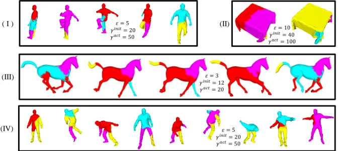
Spatio-temporal segmentation results. Figure 5 shows some sam-ples of the spatio-temporal segmentation results of our experimen-tal data (more results can be found in our supplemenexperimen-tal materials). As can be seen in this figure, given the maximal number of spatial segments (groups) ω = 4, our model is able to automatically de-termine the optimal number of vertex groups (i.e., exploiting the spatial redundancy) for different dynamic behaviors (i.e., exploiting the temporal redundancy) for all the data. For example:

• The segmentation results of the ‘March’ and the ‘Jump’ data are representatives of the local dynamic behaviors of different mesh regions. As can be seen in Figure 5, our segmentation model can not only automatically determine the number of segments, but also divide the mesh based on the local movements and group the disconnected regions with similar behaviors.

• The ‘Cloth’ animation in Figure 5(II) is firstly segmented into 4 different highly deformed regions while dropping onto the table. Then, our approach generated 3 segments, i.e., 2 waving corner regions with deformed wrinkles and 1 relatively static region. • From the segmentation results of the ‘Horse’ animation in

Fig-ure 5(III), we can observe the 4 leдs are classified into the same group when moving towards the same direction; otherwise, they form different spatial groups. Similarly, the ‘tail’ is grouped with the ‘trunk’ region in the case of the absence of distinct move-ments, or it is divided into two groups if bended.

Parallel computing. As presented in Section 4.3, the actual tempo-ral segmentation is applied to each spatial segment independently, which can be accelerated through parallel computing. In this exper-iment, we implement the actual temporal segmentation step with parallel computing on 4 cells. The computational time is shown in the column ‘sp’ in Table 1. Compared to the single thread im-plementation (column ‘s’ in Table 1), the average efficiency has been improved by 10.71%, while it can be improved even up to 35.48% (‘Cloth’ data). It is noteworthy that the decompression time is less than 0.3s for ‘March’, ‘Jump’ and ‘Handstand’, less than 0.06s for ‘Horse’ and ‘Cloth’, and less than 0.65s for ‘Flag’. This is im-portant for applications that require a fast decompression such as bandwidth-limited animation rendering and display.

Compression results. Table 1 shows the different configurations of our spatio-temporal segmentation approach for the compression of the experimental data (µ = 0.99). For each of the data with different parameters, we highlight the best ‘Rate’, ‘KGError’, and ‘Timing’ in bold fonts. We present and discuss the compression results in reference to the following parameters:

• ϵ. It is a smoothing parameter for the initial temporal segmen-tation (Section 4.1). This parameter can be empirically chosen based on the target frame rate and the mesh complexity. • γinit. If we increase γinit for the initial temporal segmentation,

the computing time may be significantly increased since the time complexity of the initial temporal segmentation (Section 4.1) is O(|γinit|2). On the other hand, its influence on KGError is limited.

Moreover, bpv f tends to decrease for most of the experimental data (except the ‘Handstand’ data).

• γact. As can be seen in Table 1, the change of γact does not significantly affect any of bpv f , KGError, and the computing time. This is because most of the actual temporal segmentation boundaries are found before reaching γact.

• ω. By increasing ω from 4 to 8, we do not observe the significant changes of the evaluation metrics. This is because our 2-stages spatial segmentation can automatically converge to the optimal number of spatial segments. Moreover, the multi-thread imple-mentation of our approach significantly improves the computa-tional efficiency (see the ‘Timing’ column in Table 1). Therefore, in general ω tends to be set to a small number. In fact, based on the previous studies [Karni and Gotsman 2004; Luo et al. 2013], ω cannot be a big number because the bit rate will increase sharply due to the additional groups’ basis. In our experiments, we empir-ically set ω= 4 because our experimental computer has a CPU of 4 cells.

5.3 Comparative Studies

We also compared our method with the method in [Sattler et al. 2005] (called as and the ‘Original Simple’ method in this writing), which is a non-sequential processing compression method. Addi-tionally, we adopted the idea in [Lalos et al. 2017] which cuts an animation into temporal blocks of the same size. Then, we can simu-late the sequential processing of the existing compression methods, including the ‘Original Soft’ in [Karni and Gotsman 2004] and the PCA-based methods, to compress each block in order. We call the adapted approaches as the ‘Adapted Soft’ and the ‘Adapted PCA’. In order to make fair comparisons, the block size of the adapted methods is approximately set to the average of |ατ | for each of the experimental data. Note that we have not included an ‘Adapted Simple’ method, which can be obtained by similarly adapting the ‘Original Simple’ method, into the comparison due to the extremely high computational cost of the ‘Original Simple’ method [Sattler et al. 2005], which is unsuitable for sequential processing.

KG Error versus bpvf. Figure 6 shows the comparisons of an ex-ample between our method and the other methods. As can be seen from this figure, our method shows a significantly better perfor-mance than the adapted methods. That is, with the same bpv f in the range of [2, 6.5], our method can always reconstruct the ‘Cloth’ animation with a much smaller KG Error. Note that the ‘Original Soft’ method has a better performance when bpv f < 2. This is because the ‘Cloth’ data contains a large portion of nearly static poses, which means the animation has significant temporal redundancies. Thus, the non-sequential precessing method (‘Orig-inal Soft’) takes this advantage by treating the entire animation. However, our method runs much more efficiently: on average, 14.5 seconds consumed by our method, 32.5 seconds consumed by the ‘Original Soft’ method, and 4421.9 seconds consumed by the ‘Orig-inal Simple’ method. Moreover, our method also provides a fine option for users who prefer high qualities after compression with slightly more storage cost, e.g., bpv f > 2.

Reconstruction errors. Figure 7 shows the heat-map visualizations of the reconstruction errors by our method and the other methods.

(9)

( I )

(II)

(III)

(IV)

𝜀 = 5 𝛾𝑖𝑛𝑖𝑡_{= 20} 𝛾𝑎𝑐𝑡_{= 50} 𝜀 = 5 𝛾𝑖𝑛𝑖𝑡_{= 20} 𝛾𝑎𝑐𝑡_{= 50} 𝜀 = 3 𝛾𝑖𝑛𝑖𝑡_{= 12} 𝛾𝑎𝑐𝑡_{= 20} 𝜀 = 10 𝛾𝑖𝑛𝑖𝑡_{= 40} 𝛾𝑎𝑐𝑡_{= 100}

Figure 5: The spatio-temporal segmentation results of the experimental data: (I)‘March’, (II)‘Cloth’, (III)‘Horse’, (IV)‘Jump’. Note that colors only indicate the intra-segment (not inter-segment) disparities. See more results in the supplemental materials.

Figure 6: Comparisons on the ‘Cloth’ animation between our model (ω = 4,γinit = 40,γact = 100) and the ‘Adapted Soft’ (block size = 100), the ‘Adapted PCA’ (block size = 100), and the ‘Original Soft’.

Overall, our method can achieve smaller reconstruction errors with lower bpvfs for the experimental data. We describe the comparative results in details as follows:

• Comparisons with the adapted methods. As can be seen in the left and the middle of Figure 7, high reconstruction errors occur randomly on the mesh using the ‘Adapted Soft’ method, as it is based on the linear prediction coding, which does not explicitly constrain the spatial affinities. For the ‘Adapted PCA’ method, high reconstruction errors occur in the regions of the vertices with rapid movements.

• Comparisons with the non-sequential processing methods. As can be seen in the right of Figure 7, for the ‘Cloth’ data, the ‘Original Soft’ method behaves with similar symptoms as the ‘Adapted Soft’ method. The ‘Original Simple’ method returns high recon-struction errors on the table-top region because this method groups the vertex trajectories based on the entire mesh sequence,

which constrains neither the temporal affinities in the local tem-poral subsequences nor the local spatial affinities. In addition, our method is significantly faster than the ‘Original Soft’ method and the ‘Original Simple’ method: our method consumed 17.78 seconds, the ‘Original Soft’ consumed 36.88 seconds, and the ‘Original Simple’ consumed 4622.36 seconds.

• Our method. Based on the above findings, our method avoids local extreme reconstruction errors using the specially-designed spatio-temporal segmentation to exploit both the spatial and the temporal redundancies. This advantage becomes more signif-icant when periodically dynamic behaviors either spatially or temporally occur in the animation. In addition, our method runs much more efficiently, compared to the non-sequential methods (i.e., ‘Original Soft’ and ‘Original Simple’).

5.4 Limitations

The main limitation of our current model is the configuration of the parameters needed for the spatio-temporal segmentation scheme. To investigate this issue, we have conducted experimental analysis on the parameters in Section 5.2. Based on our analysis, the tuning of the parameters only has limited influence on the compression results. Using the ‘Horse’ data in Table 1 as an example, the com-pression does not change when we modify γactfrom 20 to 30. This is because our approach often detects a temporal segmentation boundary before reaching γact, case (II) in Section 4.5.

Another limitation of our model is the computational cost. Al-though we have implemented some parts of our spatio-temporal segmentation model through parallel computing and its compu-tational time is superior to those of the existing non-sequential processing based compression methods, it requires further design for a frame-by-frame segmentation update scheme towards the real-time compression of 3D mesh animations in the future.

(10)

‘Our method’

‘Adapted Soft’ ‘Original Soft’

‘Original Simple’ ‘Adapted PCA’ ‘Cloth’ ‘Horse’ ‘March’ max min bpvf=5.03 KG Error=3.62 bpvf=10.66 KG Error=2.62 bpvf=9.66 KG Error=1.88 bpvf=7.69 KG Error=5.86 bpvf=5.24 KG Error=3.77 bpvf=4.62 KG Error=0.51 bpvf=10.02 KG Error=2.56 bpvf=4.63 KG Error=1.26 bpvf=4.96 KG Error=0.84

Figure 7: The reconstruction errors of the compression by using our method, ‘Adapted Soft’, ‘Adapted PCA’, ‘Original Soft’ [Karni and Gotsman 2004] and the ‘Original Simple’ [Sattler et al. 2005]. The colorbar indicates the reconstruction er-rors from low (blue) to high (red).

6 CONCLUSION

In this paper, we present a new 3D mesh animation compression model based on spatio-temporal segmentations. Our segmentation scheme utilizes a stages temporal segmentation and a two-stages vertex clustering, which are greedy processes to exploit the temporal and spatial redundancies, respectively. The main advan-tage of our scheme is the automatic determination of the optimal number of temporal segments and the optimal number of vertex groups based on global motions and the local movements of in-put 3D mesh animations. That is, our segmentation scheme can automatically optimize the temporal redundancies and the spatial redundancies for compression. Our experiments on various anima-tions demonstrated the effectiveness of our compression scheme. In the future, we would like to extend our spatio-temporal segmen-tation scheme to handle various motion represensegmen-tations, which can be potentially used for various motion-based animation searching, motion editing, and so on.

ACKNOWLEDGMENTS

This work has been in part supported by the National Natural Science Foundation of China (No.61602222, 61732015, 61762050, 61602221), the Natural Science Foundation of Jiangxi Province (No.20171BAB212011) and the Key Research and the Development Program of Zhejiang Province (No. 2018C01090), and US NSF IIS-1524782.

REFERENCES

Andreas A Vasilakis and Ioannis Fudos. 2014. Pose partitioning for multi-resolution segmentation of arbitrary mesh animations. Computer Graphics Forum 33, 2 (2014), 293–302.

Marc Alexa and Wolfgang Müller. 2000. Representing Animations by Principal Com-ponents. Computer Graphics Forum 19, 3 (2000), 411–418.

Jernej Barbič, Alla Safonova, Jia-Yu Pan, Christos Faloutsos, Jessica K. Hodgins, and Nancy S. Pollard. 2004. Segmenting Motion Capture Data into Distinct Behaviors. In Proceedings of Graphics Interface 2004 (GI ’04). Canadian Human-Computer Communications Society, School of Computer Science, University of Waterloo, Waterloo, Ontario, Canada, 185–194.

Jiong Chen, Yicun Zheng, Ying Song, Hanqiu Sun, Hujun Bao, and Jin Huang. 2017. Cloth compression using local cylindrical coordinates. The Visual Computer 33, 6-8 (2017), 801–810.

Frederic Cordier and Nadia Magnenat-Thalmann. 2005. A Data-Driven Approach for Real-Time Clothes Simulation. Computer Graphics Forum 24, 2 (2005), 173–183. Edilson de Aguiar, Christian Theobalt, Sebastian Thrun, and Hans-Peter Seidel. 2008.

Automatic Conversion of Mesh Animations into Skeleton-based Animations. Com-puter Graphics Forum 27, 2 (2008), 389–397.

Dian Gong, Gérard Medioni, Sikai Zhu, and Xuemei Zhao. 2012. Kernelized tempo-ral cut for online tempotempo-ral segmentation and recognition. In Proc. of European Conference on Computer Vision. Springer, 229–243.

Qin Gu, Jingliang Peng, and Zhigang Deng. 2009. Compression of human motion capture data using motion pattern indexing. Computer Graphics Forum 28, 1 (2009), 1–12.

Igor Guskov and Andrei Khodakovsky. 2004. Wavelet Compression of Parametrically Coherent Mesh Sequences. In Proceedings of the 2004 ACM SIGGRAPH/Eurographics Symposium on Computer Animation (SCA ’04). Eurographics Association, Goslar Germany, Germany, 183–192.

Toshiki Hijiri, Kazuhiro Nishitani, Tim Cornish, Toshiya Naka, and Shigeo Asahara. 2000. A spatial hierarchical compression method for 3D streaming animation. In Proc. of Symposium on Virtual Reality Modeling Language. 95–101.

Thomas Hofmann, Bernhard Scholkopf, and Alexander J Smola. 2008. Kernel methods in machine learning. Annals of Statistics 36, 3 (2008), 1171–1220.

Junhui Hou, Lap Pui Chau, Nadia Magnenat-Thalmann, and Ying He. 2017. Sparse Low-Rank Matrix Approximation for Data Compression. IEEE Transactions on Circuits & Systems for Video Technology 27, 5 (2017), 1043–1054.

(11)

Doug L. James and Christopher D. Twigg. 2005. Skinning Mesh Animations. ACM Trans. Graph. 24, 3 (July 2005), 399–407.

Zachi Karni and Craig Gotsman. 2004. Compression of soft-body animation sequences. Computers & Graphics 28, 1 (2004), 25–34.

Ladislav Kavan, Peter-Pike J. Sloan, and Carol O’Sullivan. 2010. Fast and Efficient Skinning of Animated Meshes. Computer Graphics Forum 29, 2 (2010), 327–336. Aris S. Lalos, Andreas A. Vasilakis, Anastasios Dimas, and Konstantinos Moustakas.

2017. Adaptive compression of animated meshes by exploiting orthogonal iterations. The Visual Computer 33, 6-8 (2017), 1–11.

Binh Huy Le and Zhigang Deng. 2014. Robust and accurate skeletal rigging from mesh sequences. ACM Transactions on Graphics 33, 4 (2014), 1–10.

Pai-Feng Lee, Chi-Kang Kao, Juin-Ling Tseng, Bin-Shyan Jong, and Tsong-Wuu Lin. 2007. 3D animation compression using affine transformation matrix and principal component analysis. IEICE Transactions on Information and Systems 90, 7 (2007), 1073–1084.

Tong Yee Lee, Yu Shuen Wang, and Tai Guang Chen. 2006. Segmenting a deforming mesh into near-rigid components. The Visual Computer 22, 9-11 (2006), 729. Xin Liu, Zaiwen Wen, and Yin Zhang. 2012. Limited Memory Block Krylov Subspace

Optimization for Computing Dominant Singular Value Decompositions. SIAM Journal on Scientific Computing 35, 3 (2012), A1641–A1668.

Guoliang Luo, Frederic Cordier, and Hyewon Seo. 2013. Compression of 3D mesh sequences by temporal segmentation. Computer Animation & Virtual Worlds 24, 3-4 (2013), 365–375.

Guoliang Luo, Gang Lei, Yuanlong Cao, Qinghua Liu, and Hyewon Seo. 2017. Joint entropy-based motion segmentation for 3D animations. The Visual Computer 33, 10 (2017), 1279–1289.

Adrien Maglo, Guillaume Lavoué, Florent Dupont, and Céline Hudelot. 2015. 3D Mesh Compression: Survey, Comparisons, and Emerging Trends. ACM Comput. Surv. 47, 3, Article 44 (Feb. 2015), 41 pages.

K. Mamou, T. Zaharia, F. Preteux, N. Stefanoski, and J. Ostermann. 2008. Frame-based compression of animated meshes in MPEG-4. In Proc. of IEEE International Conference on Multimedia and Expo. 1121–1124.

Frédéric Payan and Marc Antonini. 2007. Temporal wavelet-based compression for 3D animated models. Computers & Graphics 31, 1 (2007), 77–88.

Subramanian Ramanathan, Ashraf A. Kassim, and Tiow Seng Tan. 2008. Impact of vertex clustering on registration-based 3D dynamic mesh coding. Image & Vision Computing 26, 7 (2008), 1012–1026.

Mirko Sattler, Ralf Sarlette, and Reinhard Klein. 2005. Simple and efficient compression of animation sequences. In Proc. of ACM SIGGRAPH/Eurographics Symposium on Computer Animation. 209–217.

Alex Smola, Arthur Gretton, Le Song, and Bernhard Schölkopf. 2007. A Hilbert space embedding for distributions. In Proceeding of 18th International Conference on Algorithmic Learning Theory. Springer-Verlag, 13–31.

Nikolce Stefanoski, Xiaoliang Liu, Patrick Klie, and Jorn Ostermann. 2007. Scalable Linear Predictive Coding of Time-Consistent 3D Mesh Sequences. In 3dtv Conference. 1–4.

Nikolče Stefanoski and Jörn Ostermann. 2010. SPC: fast and efficient scalable predictive coding of animated meshes. Computer Graphics Forum 29, 1 (2010), 101–116. Robert W. Sumner and Jovan Popović. 2004. Deformation Transfer for Triangle Meshes.

ACM Trans. Graph. 23, 3 (Aug. 2004), 399–405.

Art Tevs, Alexander Berner, Michael Wand, Ivo Ihrke, Martin Bokeloh, Jens Kerber, and Hans-Peter Seidel. 2012. Animation Cartography - Intrinsic Reconstruction of Shape and Motion. ACM Trans. Graph. 31, 2, Article 12 (April 2012), 15 pages. Steven Van Vaerenbergh. 2010. Kernel methods for nonlinear identification, equalization

and separation of signals. Ph.D. Dissertation. University of Cantabria. Software available at https://github.com/steven2358/kmbox.

Libor Vasa and Vaclav Skala. 2009. COBRA: Compression of the Basis for PCA Repre-sented Animations. Computer Graphics Forum 28, 6 (2009), 1529–1540. Libor Váša and Guido Brunnett. 2013. Exploiting Connectivity to Improve the

Tangen-tial Part of Geometry Prediction. IEEE Transactions on Visualization and Computer Graphics 19, 9 (2013), 1467–1475.

Libor Váša, Stefano Marras, Kai Hormann, and Guido Brunnett. 2014. Compressing dynamic meshes with geometric laplacians. Computer Graphics Forum 33, 2 (2014), 145–154.

Daniel Vlasic, Ilya Baran, Wojciech Matusik, and Jovan Popović. 2008. Articulated Mesh Animation from Multi-view Silhouettes. ACM Trans. Graph. 27, 3, Article 97 (Aug. 2008), 9 pages.

Stefanie Wuhrer and Alan Brunton. 2010. Segmenting animated objects into near-rigid components. The Visual Computer 26, 2 (2010), 147–155.

Bailin Yang, Luhong Zhang, W.B. Frederick Li, Xiaoheng Jiang, Zhigang Deng, Meng Wang, and Mingliang Xu. 2018. Motion-aware Compression and Transmission of Mesh Animation Sequences. ACM Transactions on Intelligent Systems and Technolo-gies (2018), (accepted in December 2018).

Jeong Hyu Yang, Chang Su Kim, and Sang Uk Lee. 2002. Compression of 3-D triangle mesh sequences based on vertex-wise motion vector prediction. IEEE Transactions on Circuits & Systems for Video Technology 12, 12 (2002), 1178–1184.

Mingyang Zhu, Huaijiang Sun, and Zhigang Deng. 2012. Quaternion space sparse decomposition for motion compression and retrieval. In Proceedings of the 11th

ACM SIGGRAPH/Eurographics conference on Computer Animation. Eurographics Association, 183–192.