HAL Id: hal-02971080
https://hal.archives-ouvertes.fr/hal-02971080
Submitted on 19 Oct 2020HAL is a multi-disciplinary open access archive for the deposit and dissemination of sci-entific research documents, whether they are pub-lished or not. The documents may come from teaching and research institutions in France or abroad, or from public or private research centers.
L’archive ouverte pluridisciplinaire HAL, est destinée au dépôt et à la diffusion de documents scientifiques de niveau recherche, publiés ou non, émanant des établissements d’enseignement et de recherche français ou étrangers, des laboratoires publics ou privés.
Evaluation of liquefaction countermeasure effects on the
performance of structures
Fernando Lopez-caballero, Esteban Saez, Arézou
Modaressi-Farahmand-Razavi
To cite this version:
Fernando Lopez-caballero, Esteban Saez, Arézou Modaressi-Farahmand-Razavi. Evaluation of liq-uefaction countermeasure effects on the performance of structures. International Conference on Performance-Based Design in Earthquake Geotechnical Engineering, 2009, Tokyo, Japan. �hal-02971080�
structures
Fernando Lopez-Caballero & Esteban Saez & Arezou Modaressi-Farahmand-Razavi
Laboratoire MSS-Mat CNRS UMR 8579, Ecole Centrale Paris, France
ABSTRACT: The present paper deals with the influence of soil non-linearity, introduced by soil liquefaction, on the soil-foundation-structure interaction phenomena. Numerical simulations are carried out so as to study an improvement method to reduce the liquefaction potential in a sandy soil profile subjected to a shaking. The efficiency of the confinement walls in the mitigation of a liquefiable soil is showed. However, the interven-tion at the foundainterven-tion soil modifies the dynamic characteristics of soil-structure system and it seems to be an unfavorable method from the structural point of view.
1 INTRODUCTION
In practice, in order to mitigate the damaging effects of earthquake induced liquefaction in existing engi-neering structures, the countermeasure methods such as soil densification or diaphragm walls among oth-ers are used (Liu & Dobry 1995; Zheng et al. 1996; Adalier et al. 2003; Matsuda et al. 2005; Yasuda 2007). Such methods have been studied by several au-thors and the principal conclusion of these works is that the efficiency of each solution depends on many parameters (e.g. input signal characteristic, soil prop-erties).
According to different results, other than the ef-fects on the structure settlement, it seems that, in the case of large amplitude motion producing lique-faction phenomena in the soil foundation, the struc-tural damage in structures with significant SSI ef-fects may be reduced due to the local efef-fects (Kout-sourelakis et al. 2002; Ghosh & Madabhushi 2003; Popescu et al. 2006). Furthermore, for single-degree-of-freedom structures (SDOF) without soil structure interaction (SSI), their responses are principally in flexion mode, thus the SDOF can present great dam-age (i.e. damdam-age due to the large induced drift) re-lated to the liquefaction phenomena (Lopez-Caballero & Modaressi-Farahmand-Razavi 2008).
In the case where the mitigation method is effi-cient, it improves the properties of the soil produc-ing a soil stiffenproduc-ing effect and the liquefaction risk is eliminated. However, the damping behaviour and the frequency content modification on the surface ground motion due to liquefaction apparition are reduced and consequently the structural drift could be increased.
The aim of this work is to use numerical meth-ods in order to evaluate the efficiency of the confine-ment or diaphragm walls in the mitigation of lique-fiable loose, saturated sand to a shaking and to es-timate their effects on the earthquake motion trans-ferred to the structure through the foundation. A 2D coupled finite element modelling is carried out. The ECP’s elastoplastic multi-mechanism model, com-monly called Hujeux model (Aubry et al. 1982; Hu-jeux 1985) is used to represent the soil behavior in the numerical Gefdyn code (Aubry et al. 1986; Aubry & Modaressi 1996). A SDOF structure founded on a rigid shallow foundation is chosen to reveal, with great simplicity, the beneficial or unfavorable effects of the proposed mitigation method.
2 NUMERICAL MODEL
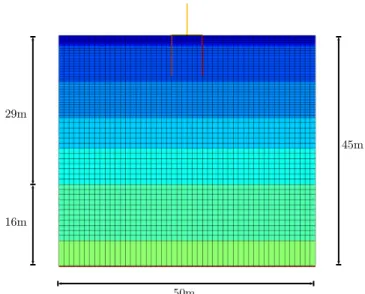
The studied site is composed principally of overcon-solidated clay layers overlaid by 29m of loose sand (i.e. a relative densityDr < 50%). According to the
test results and the soil description (Lopez-Caballero & Modaressi-Farahmand-Razavi 2008), it is deduced that the liquefaction phenomena can appear at layers between 4m and 15m depth. Thus, an elastoplastic model is only used to represent the soil behaviour on the top29m. Figure 1 shows the finite element mesh of the numerical model for the parametric study.
So as to take into account the interaction effects between the structure and the plane-strain domain, a modified “width plane strain” condition (Saez 2008) was assumed in the finite element models. In this case a width of4m is used.
50m
45m 29m
16m
Figure 1. Used finite element mesh in the numerical model.
2.1 Soil constitutive model
The ECP’s elastoplastic multi-mechanism model (Aubry et al. 1982; Hujeux 1985), commonly called Hujeux model is used to represent the soil behaviour. This model can take into account the soil behaviour in a large range of deformations. The model is writ-ten in terms of effective stress. The representation of all irreversible phenomena is made by four coupled elementary plastic mechanisms: three plane-strain de-viatoric plastic deformation mechanisms in three or-thogonal planes and an isotropic one. The model uses a Coulomb type failure criterion and the critical state concept. The evolution of hardening is based on the plastic strain (deviatoric and volumetric strain for the deviatoric mechanisms and volumetric strain for the isotropic one). To take into account the cyclic be-haviour a kinematical hardening based on the state variables at the last load reversal is used. The soil be-haviour is decomposed into pseudo-elastic, hysteretic and mobilized domains.
The model’s parameters of the soil are obtained us-ing the methodology suggested by Lopez-Caballero et al. (2007). In order to verify the model’s param-eters, the behaviour of the sand must be studied by simulating drained (DCS) and undrained cyclic shear tests (U CS). Figure 2 shows the responses of these DCS tests obtained by the model of the loose sand at σ′
mo = 40 and 80kP a. The tests results are
com-pared with the reference curves proposed by Seed et al. (1986).
The obtained curve of cyclic stress ratio (τ /σ′ m) as
a function of the number of loading cycles to produce liquefaction (N ) at σ′
m = 40kP a is given in Figure 3.
The modelled test result is compared with the refer-ence curves given by Seed & Idriss (1982) for sands at different densities (i.e.SP T values). We can notice that the obtained curve matches relatively good with
10−6 10−5 10−4 10−3 10−2 0 0.2 0.4 0.6 0.8 1 γ G/G max 10−6 10−5 10−4 10−3 10−2 0 10 20 30 40 50 γ D : % Simulation σ’ mo = 40kPa Simulation σ’ mo = 80kPa Seed et al. 1986 Simulation σ’ mo = 40kPa Simulation σ’ mo = 80kPa Seed et al. 1986
Figure 2. Comparison between simulated and refer-ence curves obtained by Seed et al. (1986).
the one corresponding toSP T − N60= 5.
100 101 102 0 0.05 0.1 0.15 0.2 0.25 N τ / σ ’ mo N 60 = 5 N60 = 10 Simulation at σ’ mo = 40kPa
Cyclic Strength Relations − Seed & Idriss (1982)
Figure 3. Comparison of simulated sand model lique-faction curves with cyclic strength relations.
2.2 Structural model
In order to simulate the single-degree-of-freedom (SDOF) structure a continuous isotropic elastic-plastic beam element is used. Non-linear structural behaviour is taken into account through an elastic-perfectly-plastic strain-stress relation. The charac-teristics of the SDOF structure used in this study are: elastic modulus, E = 25.5GP a; yielding stress of structural elements, σy = 6.0M P a; mass, M =
20000kg and height, h = 6.0m. With this character-istics the SDOF fundamental period (Tstr) is equal
to 0.4s. Concerning the seismic demand evaluation,
Figure 4 shows the corresponding capacity curve ob-tained modelling a pushover test. This curve is plot-ted using the maximum top displacement D and its corresponding base shear, in terms of spectral
accel-responds approximately to moderate-code C1L. 0 0.01 0.02 0.03 0.04 0.05 0.06 0 0.05 0.1 0.15 0.2 0.25 T el=0.4s D [m] A [g] D y=0.0051m. A y=0.128g D u=0.053m. A u=0.219g
Figure 4. Obtained SDOF Capacity Curve. Fixed base test.
As regards the confinement walls, they are com-posed of 2 inclusions with 8m depth and a thick-nesses of 0.5m. The distance between them is 6m and it is supposed that they are clamped to the foun-dation. The inclusions are simulated with continuous isotropic elastic beam elements with a Young
mod-ulus Einc = 25.5GP a (Fig. 5). They are supposed
to be impervious. The interface between the liquefi-able soil and the confinement wall was modelled us-ing “zero thickness” interface elements with a rigid-plastic Mohr-Coulomb type model. The friction angle of the interface is assumed to be23◦.
b Mass element
Beam element
Interface elements Solid elements
Figure 5. Illustration of remediation method used in the numerical model.
2.3 Input earthquake motion
The used seismic input motions are the acceleration time histories generated by a non-stationary stochas-tic simulation. The model is adapted from Pousse
acceleration, strong-motion duration, Arias intensity (Arias 1970), and central frequency. These indica-tors are empirically connected to a given database by means of ground-motion prediction equations. In our case, the European prediction equations have been used. In this work,20 synthetic earthquakes have been generated with a magnitudeMs = 7.0 and a distance
of the sourceD = 50km. The generated motions will be used as outcropping input motion with amplitudes values from0.05g to 0.20g. All signals are consistent with the response spectra of Type A soil of Eurocode8 (Fig. 6). 0 0.5 1 1.5 2 2.5 3 3.5 4 0 0.1 0.2 0.3 0.4 0.5 0.6 0.7 PSA out [g] T [s] ξ = 5% Mean ±σ Range
Figure 6. Response spectra of input earthquake mo-tions.
2.4 Boundary conditions
In the analysis, only vertically incident shear waves are introduced into the domain and as the lateral lim-its of the problem are considered to be far enough, their response is assumed to be the response of a free field. Thus, equivalent boundaries have been im-posed on the nodes of these boundaries (i.e. the nor-mal stress on these boundaries remains constant and the displacements of nodes at the same depth in two opposite lateral boundaries are the same in all direc-tions).
For the bedrock’s boundary condition, paraxial el-ements simulating a “deformable unbounded elastic bedrock” have been used (Modaressi & Benzenati 1994). The incident waves, defined at the outcropping bedrock are introduced into the base of the model af-ter deconvolution. Thus, the obtained movement at the bedrock is composed of the incident waves and the reflected signal. The bedrock is supposed to be impervious and the water level is placed at the ground surface.
3 LIQUEFACTION ANALYSIS
In order to define the liquefaction reference case, the responses obtained by the model without inclusions are analysed. Figure 7 shows the variation of peak ground acceleration (P GA) at the surface (F F ) near to the structure (i.e.12m far) and at the structure base as a function of the maximum acceleration at outcrop-ping (amax out). According to this figure, the
amplifi-cation of peak ground acceleration on the ground sur-face relative to bedrock appears beforeamax outvalue
equal to 0.12g. After this value, the non linear be-haviour of soil profile, due principally to the appari-tion of liquefacappari-tion phenomenon, produces an atten-uation of the seismic motion observed at the ground surface. 0 0.05 0.1 0.15 0.2 0 0.02 0.04 0.06 0.08 0.1 0.12 0.14 0.16 0.18 0.2 PGA [g] a max out [g] FF near SDOF Structural Base Average FF simulation
Figure 7. Relationships between maximum accelera-tions on bedrock and surface obtained in the soil pro-file.
It can be noted from the obtained pore pressure ex-cess (∆pw) in the soil profile below the foundation of
SDOF (Fig. 8), that the liquefaction zone during the 20 earthquakes is placed at layers between 2 and 8m depth.
So as to quantify the effect of the liquefaction phe-nomena, we use the computed Liquefaction Index (Q) for the profile below the foundation. This parameter is defined by Shinozuka & Ohtomo (1989) as:
Q = 1 H Z H 0 ∆pw(t, z) σ′ vo(z) dz (1)
whereH is the selected depth (in this case, H = 16m),
∆pw(t, z) is the pore water pressure build-up
com-puted at time t and depth z and σ′
vo(z) is the initial
effective vertical stress at depth z. Figure 9 provides the variation ofQ value at the end of shaking with the the Arias intensity at outcropping (IArias out). In this
study, the end of shaking is defined as the time t that corresponds to the 95% of Arias intensity t95%IArias.
0 20 40 60 80 100 120 −16 −14 −12 −10 −8 −6 −4 −2 0 Depth [m] ∆ p w [kPa] ←σ’ v0
Figure 8. Obtained pore pressure excess in the soil profile below the foundation; evolution of maximum value with depth.
Referring again to Figure 9, it can be seen that as expected, the Q value increases with an increase in IArias out value. It appears that IArias out value
pro-vides a good correlation with the thickness of the zones where liquefaction takes place (i.e. the lique-faction index). 0 0.1 0.2 0.3 0.4 0.5 0 0.05 0.1 0.15 0.2 0.25 0.3 0.35 0.4 0.45 0.5 I Arias out [m/s] Liquefaction Index, Q H=16m [.]
Figure 9. Obtained Liquefaction Index (Q) below the foundation as a function of IArias out in non linear
analyses for all cases.
As far as it concerns the relative co-seismic set-tlement induced by the liquefaction and according to Figure 10, it can be noted that, the higher Q value the higher induced settlement. According to Yasuda (2007), the large settlement induced is produced prin-cipally by the horizontal movement of the ground un-der the structure.
Regarding the response of soil structure system, according to the transfer function at FF (i.e. ratio of the frequency response at the soil surface over
0 0.1 0.2 0.3 0.4 0.5 0 1 2 3 4 5 6 7 8 Relative settlement [cm] Liquefaction Index, Q H=16m [.]
Figure 10. Variation of obtained relative settlement as a function of Liquefaction Index (Q) below the foun-dation.
the bedrock frequency response), the first natural fre-quency of the soil profile fsoil is found to be, for the
linear elastic case, at 1.75Hz (i.e. Tsoil = 0.57s). As
expected, the SDOF (fstr= 2.5Hz), being more rigid
than the soil (i.e. fsoil < fstr), presents an important
interaction with the soil foundation.
Finally, with regard to seismic demand evalua-tion on the SDOF, the maximum top displacement D and its corresponding spectral acceleration A ob-served during the ISS computation are presented in Figure 11. In this figure, the corresponding capac-ity curve obtained by modelling the pushover test is also plotted. According to this figure, it is noted that a structural non-linear behaviour appears (i.e.D > Dy,
where Dy is the displacement corresponding to the
yield capacity of structure). If µ is defined as the ductility ratio (µ = D/Dy, with Dy = 0.51cm from
pushover test), in our cases the ductility ratio varies
from1.8 to 4.8.
4 ANALYSIS OF LIQUEFACTION
IMPROVE-MENT METHODS
In this section, a mitigation method (i.e. confinement walls) is used in order to improve the ground under the SDOF structure to prevent liquefaction. The se-lected mitigation method reduces the liquefaction po-tential stiffening the soil and decreases the settlement reducing the horizontal movement of soil.
The distribution of computed normalized pore pres-sure ratio (Ru = ∆pw/σzo′ ) below the foundation at
the end of shaking for one case with and without in-clusions are shown in Figure 12. A comparison of distribution ofRu into two profiles indicates that,
be-low the foundation the level ofRu decreases strongly
when the inclusions are used. However, outside of the inclusions area, i.e. at the free field, theRuvalues are
0 0.01 0.02 0.03 0.04 0.05 0.06 0 0.5 1 1.5 2 D [m] A [m/s 2 ] ← D y
Figure 11. Structural dynamic response obtained for the SDOF compared with the static capacity curve. near to1.0 in both cases and the liquefaction phenom-ena appears.
Now, comparing the induced maximum shear strain at different depths of the profile below the foundation for the same input signal (Fig. 13), it is interesting to note that near the surface level, the cyclic shear strain values decrease when the inclusions are used. On the other hand, an opposite behaviour is observed in the soil below the inclusions. Thus, it confirms that the mitigation efficiency is due to the soil stiffening ef-fect. 0.2 0.2 0.2 0.2 0.5 0.5 0.5 0.5 0.5 0.5 0.5 0.5 0.8 0.8 0.8 0.8 0.8 0.8 0.9 0.9 15 20 25 30 35 −10 −5 0 0.2 0.2 0.2 0.5 0.5 0.5 0.5 0.5 0.5 0.5 0.8 0.8 0.8 0.8 0.8 0.8 0.8 0.8 0.8 0.9 0.9 0.9 0.9 0.9 0.9 1 1 1 1 1 Ru = ∆ p w/σ’z 0 at t = t95% I Arias 15 20 25 30 35 −10 −5 0
Figure 12. Comparison of the distribution of excess pore pressure ratio (Ru= ∆pw/σzo′ ), for one case with
(below) and without (above) inclusions.
In order to quantify the mitigation efficiency of the different configurations, the computed Liquefaction Index (Q) below the foundation for the profile with and without inclusions are compared (Fig. 14). It can be seen that the Q values decrease when the soil is improved. However, it is noted that in some cases,
0 0.005 0.01 −16 −14 −12 −10 −8 −6 −4 −2 0 Depth [m] γmax [.] 0 10 20 30 40 −16 −14 −12 −10 −8 −6 −4 −2 0 τmax [kPa] No Mitigation Mitigation
Figure 13. Induced maximum shear strain γmax and
maximum shear stressτmax on the soil profile for one
case with and without inclusions.
the value ofQ obtained after soil mitigation is greater than the reference case.
0 0.1 0.2 0.3 0.4 0.5 0 0.05 0.1 0.15 0.2 0.25 0.3 0.35 0.4 0.45 0.5 I Arias out [m/s] Liquefaction Index, Q H=16m [.] No Mitigation Mitigation
Figure 14. Comparison of Liquefaction Index (Q) ob-tained below the foundation as a function ofIArias out
for the profile with and without inclusions.
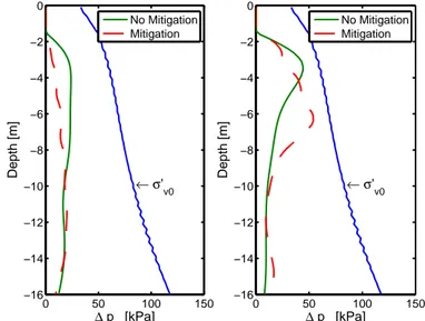
Figure 15 provides a comparison of pore pressure excess∆pw profile in two cases, when the mitigation
is efficient and when it is not. In the second case, even if the inclusion reduces the ∆pw at the soil surface
level (i.e. above4m) in relation to the reference case, it produces a pore pressure build up between 5 and 7m depth (Fig. 15). It means that the mitigation effi-ciency is a function of the inclusion stiffness and the soil around it.
As already mentioned, the remediation method used increases the liquefaction strength and decreases the settlement of the structure. As illustrated in Figure 16, the co-seismic structural settlement obtained after soil improvement is greatly reduced as a consequence
0 50 100 150 −16 −14 −12 −10 −8 −6 −4 −2 0 Depth [m] ∆ p w [kPa] ←σ’ v0 0 50 100 150 −16 −14 −12 −10 −8 −6 −4 −2 0 Depth [m] ∆ p w [kPa] ←σ’ v0 No Mitigation Mitigation No Mitigation Mitigation
Figure 15. Comparison of pore pressure excess in the soil profile obtained below the foundation for the pro-file with and without inclusions.
of soil stiffening. 0 0.1 0.2 0.3 0.4 0.5 0 1 2 3 4 5 6 7 8 9 10 Liquefaction Index, Q H=16m [.] Co−seismic Settlement [cm] No Mitigation Mitigation
Figure 16. Scatter plot of relative settlement as a func-tion of Liquefacfunc-tion Index (Q) below the foundafunc-tion with and without mitigation.
The beneficial or unfavorable effects of the miti-gation methods on the structural behaviour could be illustrated comparing the responses obtained for the profile with and without inclusions using relative ra-tios such as:∆Q = (Qmit−Qo)/Qofor the
liquefac-tion potential and∆µ = (µmit−µo)/µofor structural
behaviour. Wheremit and o subscripts refer to values after and before mitigation respectively.
In order to evaluate the effect of the introduction of the improvement methods of liquefaction on the be-haviour of the superstructure, the scatter plot of Fig-ure 17 is provided. It should be noted that, concerning the increase of pore water pressure, it is reduced by the presence of the inclusions (i.e.∆Q ≤ 0, zones II and III), thus it is a beneficial method concerning the
that in some cases, it increases because of the soil stiffening effect (i.e. ∆µ ≥ 0, zones I and II), hence it is an unfavorable method from the structural point of view. Thus, judging from these results, in addition to soil improvement it is also necessary to strengthen the structure in order to prevent its higher damage.
−50 −40 −30 −20 −10 0 10 20 30 −15 −10 −5 0 5 10 15 20 ∆ Q = (Q mit − Qo)/Qo [%] ∆ µ = ( µ mit − µ o )/ µ o [%] I II III IV
Figure 17. Scatter plot of variation of ductility
ra-tio∆µ with respect to variation of liquefaction index
∆Q.
5 CONCLUSIONS
A series of finite element parametric analyses were used to investigate the effects of the liquefaction countermeasure methods on the behaviour of exist-ing structures. A typical soil-structure model has been used to illustrate key results from parametric studies. The main conclusions drawn from this study are as follows:
1. According to the responses obtained with the model without mitigation, it can be concluded that the choice of the “bedrock” signal remains the most subtle parameter in order to define the liquefiable zones and the characteristics of possi-ble countermeasure methods. Thus, a parametric analysis is needed in order to study the influence of several signal parameters on the response of the site soil profile.
2. The analyses showed that the use of the vertical inclusions reduces the excess pore pressure ra-tio underneath the structure. The mitigara-tion effi-ciency is due to the soil stiffening effect allowing to reduce the structural settlement.
3. As far as it concerns the effect of soil improve-ment on the structural behaviour, it appears that
method from the structural point of view. As a result, it is necessary to strengthen the structure in order to prevent its collapse.
ACKNOWLEDGEMENTS
This study has been done in the framework of both the European Community Contract No GRDI-40457, NEMISREF (New methods of mitigation of seismic risk on existing foundations) and the French project
ANR-06-CATT-003-01, BELLE-PLAINE.
REFERENCES
Adalier, K., Elgamal A.-W., Meneses J., & Baez J. I. 2003. Stone columns as liquefaction countermea-sure in non-plastic silty soils. Soil Dynamics and
Earthquake Engineering 23(7), 571–584.
Arias, A. 1970. A mesure of earthquake intensity. In
Seismic Design for Nuclear Power Plants, pp. 438–
483. R.J. Hansen (ed.), MIT Press, Cambridge, Massachusetts.
Aubry, D., Chouvet D., Modaressi A., & Moda-ressi H. 1986. GEFDYN: Logiciel d’Analyse de Comportement M´ecanique des Sols par El´ements Finis avec Prise en Compte du Couplage Sol-Eau-Air. Manuel scientifique, Ecole Centrale Paris, LMSS-Mat.
Aubry, D., Hujeux J.-C.,Lassoudi`ere F., & Meimon Y. 1982. A double memory model with multiple mech-anisms for cyclic soil behaviour. In Int. Symp. Num.
Mod. Geomech, pp. 3–13. Balkema.
Aubry, D. & Modaressi A. 1996. GEFDYN. Manuel scientifique, Ecole Centrale Paris, LMSS-Mat. Ghosh, B. & Madabhushi S. P. G. 2003. Effects of
localised soil inhomogenity in modyfyng seismic soil structure interaction. In 16th ASCE
Engineer-ing Mechanics Conference. University of WashEngineer-ing-
Washing-ton, Seattle.
Hujeux, J.-C. 1985. Une loi de comportement pour le chargement cyclique des sols. In G´enie
Parasis-mique, pp. 278–302. V. Davidovici, Presses ENPC,
France.
Koutsourelakis, S., Pr´evost J. H., & Deodatis G. 2002. Risk assessment of an interacting structure-soil sys-tem due to liquefaction. Earthquake Engineering
and Structural Dynamics 31(4), 851–879.
Liu, L. & Dobry R. 1995. Effect of liquefaction on lat-eral response of piles by centrifuge model tests.
Na-tional Center for Earthquake Engineering Research (NCEER) Bulletin 9(1), 7–11.
Lopez-Caballero, F. & Modaressi-Farahmand-Razavi A. 2008. Numerical simulation of liquefaction ef-fects on seismic SSI. Soil Dynamics and
Lopez-Caballero, F., Modaressi-Farahmand-Razavi A., & Modaressi H. 2007. Nonlinear numerical method for earthquake site response analysis i- elastoplas-tic cyclic model & parameter identification strategy.
Bulletin of Earthquake Engineering 5(3), 303–323.
Matsuda, T., Tanaka K., & Okano M. 2005. Advanced in-service seismic retrofitting methods for a railway viaduct. In Proccedings 1st Greece-Japan
Work-shop : Seismic design, observation and retrofit of foundations, Athens, pp. 277–287. Gazetas et al.
Eds.
Modaressi, H. & Benzenati I. 1994. Paraxial approx-imation for poroelastic media. Soil Dynamics and
Earthquake Engineering 13(2), 117–129.
Popescu, R., Pr´evost J. H., Deodatis G., & Chakrabortty P. 2006. Dynamics of nonlinear porous media with applications to soil liquefaction. Soil Dynamics and
Earthquake Engineering 26(6-7), 648–665.
Pousse, G., Bonilla F., Cotton F., & Margerin L. 2006. Non stationary stochastic simulation of strong ground motion time histories including natural vari-ability: Application to the K-net Japanese database.
Bulletin of the Seismological Society of Amer-ica 96(6), 2103–2117.
Saez, E. 2008. Dynamic non-linear Soil-Structure
Inter-action. PhD thesis, ´Ecole Centrale Paris, France. Seed, H. B. & Idriss I. M. 1982. Ground motion and soil
liquefaction during earthquakes. Monograph series, earthquake engineering research institute, Univer-sity of California, Berkeley, CA.
Seed, H. B., Wong R. T., Idriss I. M., & Tokimatsu K. 1986. Moduli and damping factors for dynamic analyses of cohesionless soils. Journal of
Geotech-nical Engineering - ASCE 112(11), 1016–1032.
Shinozuka, M. & Ohtomo K. 1989. Spatial severity of liquefaction. In Proceedings of the second
US-Japan workshop in liquefaction, Large Ground De-formation and Their Effects on Lifelines.
HAZUS-MH MR3 2003. Multi-hazard Loss Estimation Methodology. Technical Manual. Report FEMA, Federal Emergency Management Agency.
Yasuda, S. 2007. Remediation methods againts lique-faction which can be applied to existing structures. In Earthquake Geotechnical Engineering, pp. 385– 406. K.D. Pitilakis Ed., Springer, The Netherlands. Zheng, J., Suzuki K., Ohbo N., & Prevost J.-H.
1996. Evaluation of sheet pile-ring countermeasure against liquefaction for oil tank site. Soil Dynamics