HAL Id: hal-03135932
https://hal.inria.fr/hal-03135932
Submitted on 9 Feb 2021
HAL is a multi-disciplinary open access
archive for the deposit and dissemination of
sci-entific research documents, whether they are
pub-lished or not. The documents may come from
teaching and research institutions in France or
abroad, or from public or private research centers.
L’archive ouverte pluridisciplinaire HAL, est
destinée au dépôt et à la diffusion de documents
scientifiques de niveau recherche, publiés ou non,
émanant des établissements d’enseignement et de
recherche français ou étrangers, des laboratoires
publics ou privés.
Constant overhead quantum fault tolerance with
quantum expander codes
Omar Fawzi, Antoine Grospellier, Anthony Leverrier
To cite this version:
Omar Fawzi, Antoine Grospellier, Anthony Leverrier. Constant overhead quantum fault tolerance
with quantum expander codes. Communications of the ACM, Association for Computing Machinery,
2021, 64 (1), pp.106-114. �10.1145/3434163�. �hal-03135932�
research highlights
Constant Overhead Quantum
Fault Tolerance with Quantum
Expander Codes
By Omar Fawzi, Antoine Grospellier, and Anthony Leverrier
DOI:10.1145/3434163
Abstract
The threshold theorem is a seminal result in the field of quantum computing asserting that arbitrarily long quan-tum computations can be performed on a faulty quanquan-tum computer provided that the noise level is below some con-stant threshold. This remarkable result comes at the price of increasing the number of qubits (quantum bits) by a large factor that scales polylogarithmically with the size of the quantum computation we wish to realize. Minimizing the space overhead for fault-tolerant quantum computation is a pressing challenge that is crucial to benefit from the compu-tational potential of quantum devices.
In this paper, we study the asymptotic scaling of the space overhead needed for fault-tolerant quantum computation. We show that the polylogarithmic factor in the standard threshold theorem is in fact not needed and that there is a fault-tolerant construction that uses a number of qubits that is only a constant factor more than the number of qubits of the ideal computation. This result was conjectured by Gottesman who suggested to replace the concatenated codes from the standard threshold theorem by quantum error-correcting codes with a constant encoding rate. The main challenge was then to find an appropriate family of quantum codes together with an efficient classical decod-ing algorithm workdecod-ing even with a noisy syndrome. The effi-ciency constraint is crucial here: bear in mind that qubits are inherently noisy and that faults keep accumulating during the decoding process. The role of the decoder is therefore to keep the number of errors under control during the whole computation.
On a technical level, our main contribution is the analy-sis of the small-set-flip decoding algorithm applied to the family of quantum expander codes. We show that it can be parallelized to run in constant time while correct-ing sufficiently many errors on both the qubits and the syndrome to keep the error under control. These tools can be seen as a quantum generalization of the bit-flip algo-rithm applied to the (classical) expander codes of Sipser and Spielman.
1. INTRODUCTION
Quantum computers are expected to offer significant, sometimes exponential, speedups compared to classi-cal computers. For this reason, building a large, universal quantum computer is a central objective of modern science.
The original version of this paper was published in FOCS 2018.
Despite two decades of effort, experimental progress has been somewhat slow and the largest computers available at the moment reach a few tens of physical qubits, still quite far from the numbers necessary to run “interesting” algo-rithms. A major source of difficulty is the extreme fragility of quantum information: storing a qubit is very challenging, but processing quantum information even more so.
Any physical implementation of a quantum computer is unavoidably imperfect because qubits are subject to decoherence and physical gates can only be approxi-mately realized. In order to compute the outcome of an ideal circuit C using imperfect qubits and gates, the idea is to transform C into another circuit C¢, which gives the same outcome with high probability, even if its compo-nents are noisy. It is common to refer to the gates or wires of the circuit C as logical gates or wires and to those of C¢ as the physical ones.
1.1. Fault-tolerant classical computation
The idea of constructing reliable circuits from unreliable components goes back to von Neumann25 and we briefly
sketch the construction he proposed. Given an ideal clas-sical circuit C computing a Boolean function, we construct C¢ by duplicating each wire and each gate m times. For exam-ple, suppose we have an and gate between wires w1 and w2 in C. Then, we will associate to the logical wires wb in C, m physical wires for i ∈ {1, . . . , m}, and the logical and will be implemented by m physical and gates between wires and . Then, the output of C¢ is defined as the majority applied to the m wires corresponding to the output of C. If the components of C¢ are perfect, we can see C¢ as a version of C where each wire is encoded in a simple error-correcting code: the m-repetition code. If the components of C¢ are now noisy, then the m wires will generally take different values. As each gate can potentially propagate errors, it is important to correct for errors regularly. If we could apply perfect gates, this would be easy: we simply apply a majority vote among the m wires. Interestingly, von Neumann showed the exis-tence of a circuit that reduces errors even with noisy gates and he called it a “restoring organ.” This is done by apply-ing majorities not on all the m wires but on well-chosen sub-sets using a concentrator; see Pippenger16 for details. As the
probability that the majority of a block of m wires takes the wrong value is exponentially small in m, it is sufficient to
choose m = O(log s) to ensure that all the components of the circuit work as expected with high probability. Here,
s is the number of gates in the original circuit C. Thus,
starting with a circuit C with s gates, the circuit C¢ has O(s log s) gates.
It is very natural to ask at this point whether this logarith-mic overhead to construct a fault-tolerant circuit is best pos-sible. Instead of using a simple repetition code, we might try to encode our computation using an error-correcting code with better parameters. In fact, it is well-known since Shannon’s work18 that instead of encoding only one bit in
m wires, we could encode a number of bits that is linear in m while keeping a comparable error probability. The first
difficulty when using more complicated codes is the imple-mentation of gates. This was particularly simple for the rep-etition code as described earlier: to implement a logical and gate, it suffices to apply m and physical gates between dis-joint wires. Using the standard terminology used in quan-tum fault tolerance, we say that the repetition code has a transversal and. The important property here is that the circuit to implement a logical and gates uses a physical cir-cuit of constant depth and so errors cannot propagate too much. The second difficulty is to design an error reduction procedure using noisy gates for such general codes. In fact, it turns out that this logarithmic overhead is unavoidable as shown in Pippenger et al.17
We finally note that for classical computers, fault toler-ance is not needed in practice because with the develop-ment of the transistor, errors almost never occur.
1.2. Fault-tolerant quantum computation
On the other hand, for quantum computers, fault toler-ance is really necessary. For this reason, immediately after Shor discovered his famous factoring quantum algorithm,19
the search for methods to reduce the effect of decoherence started. Shor himself showed that, perhaps contrary to what one could infer from the quantum no-cloning principle, quantum error-correcting codes do exist20 and he made
some steps toward fault tolerance.21 A few years later, the
celebrated threshold theorem was proved. It states that upon encoding the logical qubits within the appropriate quan-tum error-correcting code, it is possible to transform an arbitrary quantum circuit C into a fault-tolerant one C¢, such that even if the components of the circuit C¢ are sub-ject to noise, below some threshold value it computes the same function as C.1
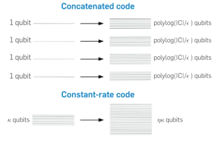
Naturally, the fault-tolerant circuit C¢ will be larger than C. In particular, a number of additional qubits are required and the space overhead, that is, the ratio between the total number of qubits of the fault-tolerant circuit C¢ and the number of qubits of the ideal circuit C, scales polylogarith-mically with the number of gates involved in the original computation. The depth and size overhead are also poly-logarithmic, but we focus here on the space overhead. The polylogarithmic factor comes for a reason that is similar to the logarithmic factor in von Neumann’s construction for the classical case. The main technique that is used to pro-tect logical qubits is to use concatenated codes. In order to guarantee an overall failure probability ε for a circuit C
acting on κ qubits with |C| locations,a the fault-tolerant
version of the circuits needs O(log log (|C|/ε)) levels of encoding, which translates into a polylog(|C|/ε) space overhead (see Figure 1).
Although this might seem like a reasonably small over-head, this remains rather prohibitive in practice. As an example, an application of Shor’s algorithm to factorize numbers of cryptographic interest would require a few thousand logical qubits, but tens of millions of physi-cal qubits with the best fault-tolerant schemes currently available; see for example, Fowler et al.6 and Gidney and
Ekerå.9 Given the extreme difficulty of controlling a large
number of qubits, it is absolutely crucial to try to reduce the overhead of quantum fault tolerance as much as pos-sible. From a computational point of view, it is also a very natural question to determine the optimal overhead required to achieve fault tolerance. As a classical com-putation is a special case of quantum comcom-putation, the previously mentioned logarithmic lower bound for fault-tolerant classical space overhead applies.17 However, in
this context, it is natural to treat classical computations and quantum computations differently. In fact, it is very well motivated in practice to assume that classical com-putations are error-free but that quantum gates are noisy and to ask what is the minimal possible space overhead that can be achieved in this setting. In this model, build-ing on Gottesman’s framework,11 we prove that
quan-tum fault tolerance is possible with constant overhead (see Theorem 1). The main tool that we introduce here in order to achieve this goal is a class of quantum error correcting with good properties. These codes are called
quantum expander codes and they are constant-rate
low-density parity-check quantum codes with a decoding algorithm that can correct typical errors very efficiently even when the syndrome is noisy (see Theorem 3). Before introducing quantum expander codes, we give an overview
1 qubit 1 qubit 1 qubit 1 qubit κ qubits ηκ qubits Constant-rate code polylog(|C|/ε ) qubits polylog(|C|/ε ) qubits polylog(|C|/ε ) qubits polylog(|C|/ε ) qubits Concatenated code
Figure 1. A natural idea to save on the memory overhead is to encode multiple qubits in the same block.
a A location is any point in the circuit that could have an error, so it refers to a quantum gate, the preparation of a qubit in a given state, a qubit measure-ment, or a wait location if the qubit is not acted upon at a given time step.
research highlights
under control is low-density parity-check (LDPC) codes. This property is crucial as it ensures that the syndrome measure-ment circuit is of constant depth and thus errors cannot propagate too much.
Another property that the quantum code needs to have is that it can correct typical errors of size linear in the block-length n. This means that the minimum distance of the code should at least grow with n. And constant rate LDPC codes with minimum distance growing with n are quite difficult to construct. The situation is indeed much more involved than in the classical case where good LDPC codes (constant rate and linear minimum distance) can be found by picking a sparse parity-check matrix at random. In the quantum case, by contrast, the best known constructions display a mini-mum distance barely above the square-root of the length
.7 But it is not sufficient to have quantum codes with
large minimum distance: the decoding algorithm needs to be efficient. In fact, efficient decoding is crucial in the con-text of fault tolerance: while the decoding algorithm is run-ning, the quantum circuit is waiting for the output of the decoding algorithm and thus errors keep accumulating. Thus, ideally, we would want the decoding to run in con-stant time that is independent of the number of qubits of the circuit. In addition to the efficiency, another impor-tant property that the decoding algorithm should have is that it should come with guarantees even if the observed syndrome σ is itself noisy. In fact, recall that the syndrome
measurement circuit will be faulty and so its outcome will have a certain number of errors.
In the present work, we consider quantum expander codes introduced in Leverrier et al.15 obtained by taking the
hyper-graph product24 of classical expander codes.22 We show
that the small-set-flip decoding algorithm introduced in Leverrier et al.15 does satisfy all these properties. Namely,
this algorithm can, in a constant number of time steps, reduce the size of a typical error by a constant fraction even if the observed syndrome is noisy.
We obtain the following general result by using our anal-ysis of quantum expander codes in Gottesman’s generic construction.11
Theorem 1. For any η >1 and ε >0, there exists pT (η) >0 such that the following holds for sufficiently large κ. Let C be a quan-tum circuit acting on κ qubits, and consisting of f (κ) locations for f an arbitrary polynomial. There exists a circuit C using ηκ phys-ical qubits, depth O( f (κ)), and number of locations O(κ f (κ)) that outputs a distribution, which has total variation distance at most ε from the output distribution of C, even if the compo-nents of C are noisy with an error rate p<pth.
2. QUANTUM EXPANDER CODES
In this section, we first review the construction of classical and quantum expander codes. We then discuss models of noise that are relevant in the context of quantum fault tol-erance. We finally introduce the small-set-flip decoding algorithm for quantum expander codes.
2.1. Classical expander codes
A linear classical error-correcting code C of of Gottesman’s fault-tolerant scheme to motivate the
desired properties of the quantum codes.
1.3. Gottesman’s scheme
The natural approach to overcome the polylogarithmic barrier had been contemplated for a while, namely to rely on quan-tum error-correcting codes that encode multiple logical qubits within a block. Ideally, we would like to encode the
κ logical qubits needed for the computation within a single
quantum error-correcting code of length n with n linear in
κ (see Figure 1) and then perform the gates
correspond-ing to the computation within this code and regularly cor-recting (or more precisely reducing) the errors. However, turning this idea into a full-fledged scheme required much more work. The two main difficulties are to implement fault- tolerantly the logical gates and to correct the errors in a fault-tolerant way. In a breakthrough paper, Gottesman was able to overcome the first difficulty and partially the second one: he showed that polynomial-time computations could be performed with a noisy circuit with only a constant over-head provided that a family of quantum codes with good decoding properties was available.11 In fact, this overhead
can even be taken arbitrarily close to 1 provided that the physical error is sufficiently small.
We start by briefly describing how Gottesman’s construc-tion dealt with the difficulty of implementing the logical gates. One special gate that is used at the beginning of the computation is a preparation gate that prepares a fixed logi-cal qubit state. We need to be able to apply this gate in a fault-tolerant way, that is, such that the number of qubits having an error is under control. In fact, using the technique of gate teleportation, once we are able to fault-tolerantly prepare a small number of fixed logical states, we can implement any logical gate in a fault-tolerant way. In order to achieve this fault-tolerant state preparation, Gottesman uses techniques based on code concatenation. But to keep the associated memory overhead small, we cannot prepare all the κ logical
qubits in one shot. Instead, the κ logical qubits of the circuit
C are partitioned into polylog(κ) blocks of qubits each and each block is encoded using a constant rate code. Then, the logical circuit C is “serialized” in such a way that a single gate is applied at each time step. In this way, at a given time step, only one gate is applied that acts on at most two logical qubits. Thus, at most two of the blocks are active and the overhead used for applying this gate is polylogarithmic in and thus still linear in κ.
The error correction part of the fault-tolerant scheme is more relevant for the present work. The standard error cor-rection procedure for a quantum error-correcting code is to perform a measurement that outputs a syndrome σ (this is
in direct analogy with classical error-correcting codes) and then the decoding algorithm is a classical algorithm tak-ing as input σ and returning an error E that is consistent
with this syndrome. This error E is then undone by acting on the quantum systems. We refer to Section 2.2 for formal definitions of quantum error-correcting codes. If the quan-tum components used for this measurement are noisy, the obtained syndrome will in general be incorrect. One class of codes for which the number of errors in the syndrome stays
the syndrome is potentially noisy, the goal changes a little bit because it is not possible in general to correct all errors. In that case, it is sufficient to keep the error weight under control, and this can possibly be achieved by performing a constant number of rounds instead of a logarithmic one. Our present aim is to generalize these results to the quan-tum setting.
2.2. Quantum error-correcting codes
A quantum error-correcting code encoding κ logical qubits
into n physical qubits is a subspace of (C2)⊗n of dimension
2κ. The stabilizer formalism developed by Gottesman10
allows one to describe a code as the kernel of a linear operator, exactly as in the classical case. A stabilizer group is an Abelian group 〈g1, . . . ,gm〉 of n-qubit Pauli operators (n-fold tensor products of single-qubit Pauli operators
and with an overall phase of ±1 or ±i) that does not contain −I. The associated stabilizer
code is defined as the common eigenspace of the generators g1, . . . ,gm with eigenvalue ±1. If the generators are indepen-dent, then κ = n–m.
Devising good codes is significantly more complex in the quantum case because of the commutation require-ment for the generators. A convenient way to enforce this condition is via the CSS construction,3, 23 where the
stabi-lizer generators are either products of single-qubit X-Pauli matrices or products of Z-Pauli matrices. Commutativity should then only be verified between X-type generators (corresponding to products of Pauli X-operators) and
Z-type generators, and this can be obtained directly by
considering two classical linear codes CX and CZ of length
n with parity-check matrices HX and Hz satisfying = 0. The generators of the stabilizer are of the form , and
is defined as
,
where Xj denotes the X Pauli operator applied to the jth fac-tor, and where identity operators are omitted. The resulting quantum code has length n and encodes κ = dim CX + dim CZ – n logical qubits. Its minimum distance dmin is defined in analogy with the classical case as the minimum Hamming weight of a Pauli operator mapping a code word to an orthog-onal one. For the CSS code, one has dmin= min (dX, dZ) where
and , where the dual code consists of words orthogonal to all words of CX. Note that dX can be larger than the minimum dis-tance of the classical code CX as we only consider the weight of code words in CX that are not in . In fact, for quantum LDPC codes, the minimum distance of the classical CX will be bounded by a constant because the condition
implies that the rows of HZ, which have a constant weight by the LDPC condition, are in CX. As such, to construct inter-esting quantum LDPC codes, it is crucial to use the condi-tion . The reason the bistrings in should not be considered as errors is that the corresponding X-type Pauli operators are in the stabilizer group and thus do not affect the state. Two Pauli X-type operators (e.g., errors) that are related by a Pauli X-type operator whose support is given by dimension κ and length n is a subspace of of dimension κ.
Mathematically, it can be defined as the κ-dimensional
kernel of an m×n matrix H, called the parity-check matrix of the code: . The minimum distance dmin of the code is the minimum Hamming weight of a nonzero code word: . Such a linear code is often denoted as [n, κ, dmin], and a code family has a constant
encoding rate when κ = Θ(n). An important property for a
lin-ear code is the sparsity of H: the code is a low-density
parity-check (LDPC) code when the rows and columns of H have a
weight bounded by a constant.8 This is particularly attractive
because it allows for efficient decoding algorithms, based on message passing for instance.
An alternative description of a linear code is via a bipar-tite graph known as its factor graph G = (V ∪ C, E ) and defined as follows. The sets V of bits and C of check-nodes have cardinality n and m, respectively, and an edge is present between υ ∈ V and c ∈ C whenever Hc,v = 1. In particular, any bipartite graph of constant maximum degree gives rise to an LDPC code. Depending on the description, an error is either a binary word or a subset E ⊆ V whose indicator vector is e. Its corresponding syndrome is then either or the subset corresponding to the odd neighborhood of E in the graph. Here, Γ(υ) ⊆ C is the set of
neighbors of υ and the operator ⊕ is interpreted as the
sym-metric difference of sets.
The codes that we will rely on for quantum fault tolerance are the quantum generalization of expander codes, which are the classical codes associated with expander graphs, and first considered by Sipser and Spielman.22
Definition 2 (Expander graph). Let G = (V ∪ C, E ) be a
bipartite graph with left and right degrees bounded by dV and
dC, respectively. We say that G is (γ,δ)-expanding if for any sub-set S ⊆ A (with A is equal to either V or C) with |S|≤ γ|A|, we
have .
Observe that we are requiring two-sided expansion for the graph. Even though only one-sided expansion is required for analyzing classical expander codes, the definition asks for two-sided expansion as this is used for the analysis of quantum expander codes. We note that the existence of (γ,δ) bipartite expanders can be shown via the probabilistic
method provided that and γ is a sufficiently small
constant. Remarkably, classical expander codes come with an efficient decoding algorithm, bit-flip, that can correct
arbitrary errors of weight Ω(n), provided that .22 The
strategy behind the bit-flip decoding algorithm is as sim-ple as it can get: given some observed syndrome σ(E), simply
go through the bits υ ∈ V and flip any bit υ if this decreases
the syndrome weight, that is, if | σ(E ⊕ {υ})| < |σ(E)|. For
a sufficiently expanding factor graph, and provided that the error weight is below γn, it is possible to show that there
exist critical bits satisfying the condition above, and in fact, the number of such critical bits is linear in the size of E. Going through all the bits once will therefore decrease the syndrome weight by a constant fraction, and decoding will be achieved with logarithmic depth if the algorithm is suit-ably parallelized. In the context of fault tolerance, where
research highlights
error-correcting code, replace the locations of the origi-nal circuit by gadgets applying the corresponding gate on the encoded qubits, and interleave the steps of the com-putation with error correction steps. In general, it is con-venient to abstract away the details of the implementation and consider a simplified model of fault tolerance where one is concerned with only two types of errors: errors occurring at each time step on the physical qubits, and errors on the results of the syndrome measurement. The link between the basic and the simplified models for fault tolerance can be made once a specific choice of gate set and gadgets for each gate is made. This is done for instance in Section 7 of Gottesman.11 In other words, the simplified model of fault
tolerance allows us to work with quantum error-correcting codes where both the physical qubits and the check nodes are affected by errors.
As usual in the context of quantum error correction, we restrict our attention to Pauli-type errors acting on the set
V of qubits because the ability to correct all Pauli errors of
weight t implies that arbitrary errors of weight t can be cor-rected. In particular, one only needs to address X- and Z-type errors because a Y-error corresponds to simultaneous X- and Z-errors. Therefore, we think of an error pattern on the qubits as a pair (EX, EZ) of subsets of the set of qubits V. This should be interpreted as Pauli error X on all qubits in EX \ EZ, error Y on EX ∩ EZ and error Z on EZ \ EX. In the case of a CSS code, the syndrome associated to this error pattern should be (σX(EX), σZ(EZ)) but errors will also affect the syndrome extraction, leading to an observed syndrome (σX, σZ) given by where the error on the syndrome consists of two classical strings (DX, DZ), which are subsets of the sets CX and CZ of check nodes, whose values have been flipped.
How to properly model the effect of noise in a quantum computer is a delicate question. In particular, the assump-tion of independence of errors affecting distinct qubits is not well justified because the topology of the quantum cir-cuit will generally create correlations between errors. For this reason, a particular reasonable approach suggested by Gottesman consists in only making the assumption that the probability of an error decays exponentially with its weight.11
The relevant error model for the pair (EX, DX) is the local
sto-chastic noise model with parameters (p, q) defined by
requir-ing that for any F ⊆ V and G ⊆ CX, the probability that F and
G are part of the qubit and syndrome errors, respectively, is
bounded as follows:
The error model is exactly the same for the pair (EZ, DZ). Note that, as the decoding algorithm we use does not take into account correlations between X and Z errors, the joint distri-bution between (EX, DZ) and (EZ, DZ) will not affect the analysis.
2.4. The small-set-flip decoding algorithm
If the syndrome extraction is noiseless, a decoder is given the pair (σX, σZ) of syndromes and should return a pair of an element in are called equivalent. We say that CSS(CX,CZ)
is a [[n, κ, dmin]] quantum code.
Even if the CSS framework simplifies matters a little bit, it remains nontrivial to find interesting codes subjected to the condition . The hypergraph product code construction introduced by Tillich and Zémor gives a general method to turn a pair of arbitrary linear codes into a quan-tum CSS code.24 In particular, starting with a classical code
C with parity-check matrix H and a biregular (γ,δ)-expanding
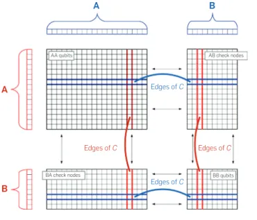
factor graph with vertex set A ∪ B (of size nA + nB) and left and right degrees dA and dB (satisfying dA ≤ dB), one obtains a CSS code called quantum expander code with parity-check matri-ces HX and HZ given by
We illustrate this construction in Figure 2.
Quantum expander codes are LDPC with generators of weight
dA + dB and qubits involved in at most 2dB generators, and they admit parameters [[n, κ, dmin]] with , provided that the expansion satisfies .
2.3. Noise models
In the context of quantum fault tolerance, we are interested in modeling noise occurring during a quantum computa-tion. In the circuit model of quantum computation, the effect of noise is to cause faults occurring at different locations of the circuit: on the initial state and ancillas, on gates (either active gates or storage gates) or on measurement gates. We refer to this model as basic model for fault tolerance. The main idea to perform a computation in a fault-tolerant manner is then to encode the logical qubits with a quantum
Figure 2. An illustration of quantum expander codes. Starting with a bipartite expander graph between the vertex sets A and B, the quantum expander code is defined by two bipartite graphs: HX between the set of qubit nodes (A × A) ∪ (B × B) and the check nodes A × B and HZ between the qubit nodes (A × A) ∪ (B × B) and
the check nodes B × A.
AA qubits BB qubits AB check nodes Edges of C A A B B Edges of C Edges of C Edges of C BA check nodes
SUCCESS: if for X ⊆ X, i.e., E and are equivalent errors ; σ0 = σ; i = 0 while do // i = i + 1 end while return
Leverrier et al.15 studied the decoding algorithm
small-set-flip and showed that it corrects arbitrary qubit errors of size for quantum expander codes (when the syn-drome extraction is noiseless) provided that the expansion of the graph satisfies .
This analysis was extended to the case of random errors (either independent and identically distributed, or local sto-chastic) provided that the syndrome extraction is performed perfectly and under a stricter condition on the expansion of the graph.5 More precisely, for quantum expander codes
with an expansion , there exist a probability p0 > 0 and constants C, C′ such that if the noise parameter on the qubits satisfies p< p0, the small-set-flip decoding algorithm described above runs in time linear in the code length and corrects a random error with probability at least .
The analysis of the decoding algorithm is inspired by the work of Kovalev and Pryadko14 who studied the behavior
of the maximum likelihood decoding algorithm (that has exponential running time in general). We represent the set of qubits as a graph G = (V, E) called adjacency graph where the vertices correspond to the qubits of the code and two qubits are linked by an edge if there is a stabilizer generator that acts on the two qubits. The approach is then to show that provided the vertices E corresponding to the error do not form large connected subsets, the error can be corrected by the decoding algorithm. How large the connected sub-sets are allowed to be is related to the minimum distance of the code for the maximum-likelihood decoder or to the maximum size of correctable errors for more general decod-ers. This naturally leads to studying the size of the largest connected subset of a randomly chosen set of vertices of a graph. This is also called site percolation on finite graphs and is a well-studied topic.
In order to analyze the efficient small-set-flip decoding algorithm for quantum expander codes, a slightly more com-plex notion of connectivity turns out to be relevant. Namely, instead of studying the size of the largest connected subset of E, one studies the size of the largest connected α-subset
of E. We say that X is an α-subset of E if |X ∩ E| ≥ α|X|. Note
that for α = 1, this is the same as X is a subset of E. Then, one
shows that, if the probability of error of each qubit is below some threshold depending on α and the degree of G, then
the probability that a random set E has a connected α-subset of size vanishes as . As small-set-flip can correct errors of size , one concludes that random errors of linear size are corrected with high probability. The errors such that and . In
that case, the decoder outputs an error equivalent to (EX, EZ), and we say that it succeeds.
A natural approach to perform error correction (in the noiseless syndrome case) would be to directly mimic the classical bit-flip decoding algorithm analyzed by Sipser and Spielman, that is try to apply X-type (or Z-type) correction to qubits when it leads to a decrease of the syndrome weight. Unfortunately, in that case, there are error configurations of constant weight that cannot be corrected in this way. This led Leverrier et al.15 to introduce the small-set-flip strategy
that we describe next.
Focusing on X-type errors for instance, and assuming that the syndrome σ = σX(E) is known, the algorithm cycles through all the X-type generators of the stabilizer group (i.e., the rows of HZ), and for each one of them, it deter-mines whether there is an error pattern contained in the generator that decreases the syndrome weight. Assuming that this is the case, the algorithm applies the error pat-tern (choosing the one maximizing the ratio between the syndrome weight decrease and the pattern weight, if there are several). The algorithm then proceeds by examining the next generator. Because the generators have constant weight dA + dB, there are 2dA+ dB = O(1) possible patterns to
examine for each generator.
Before describing the algorithm more precisely, let us intro-duce some additional notations. Let X be the set of subsets of V corresponding to X-type generators: i ∈
[m]}⊆ P(V), where P(V) is the power set of V. Here, m denotes the number of X-type generators, and denotes the subset of qubits on which acts nontrivially. The indica-tor vecindica-tors of the elements of X span the dual code . The condition for successful decoding of the X-type error E is that E equivalent to the output of the decoding algorithm , i.e., there exists a subset X ⊂ X such that . At each step, the small-set-flip algorithm tries to flip a sub-set of for some generator , which decreases the syndrome weight |σ|. In other words, it tries to flip some
ele-ment F ∈ F0 such that ∆(σ, F) > 0 where:
(1) The small-set-flip decoding algorithm consists of two iterations of Algorithm 1 below: it first tries to correct
X-type errors by examining the corresponding syndrome σX(EX), and then, it is applied a second time (exchanging the roles of X and Z) to correct Z-type errors. The idea of applying the same decoder twice, to correct first X-type errors, and then Z-type errors, is particularly natural when considering a CSS code. Note that this is a suboptimal strat-egy in general because both types of errors could be cor-related, but this will be sufficient for our purpose and this significantly simplifies the exposition.
Algorithm 1: small-set-flip for noiseless syndrome. INPUT: a syndrome σ = σX(E) ⊆ CX, corresponding to an unknown X-type error pattern E ⊆ V
research highlights
we cannot hope to recover an equivalent error exactly, but instead we can control the size of the remaining error by the amount of noise in the syndrome measurements. In particular, for any qubit error rate below p0, the decoding operation reduces this error rate to be (our choice of
p0 will be such that ). This criterion is sufficient for fault-tolerant schemes as it ensures that the size of the qubit errors stay bounded throughout the execution of the circuit. The proof of this theorem consists of two main parts: analyzing arbitrary errors of weight and then exploiting percolation theory to analyze stochastic errors of linear weight.
3.1. Sketch of the analysis
The small-set-flip decoding algorithm proceeds by try-ing to flip small sets of qubits so as to decrease the weight of the syndrome, and the main challenge in its analysis is to prove the existence of such a small set F. In the case where the observed syndrome is error free, Leverrier et al.15 and
Fawzi et al.5 relied on the existence of a “critical generator”
to exhibit such a set of qubits. This approach, however, only yields a single such set F, and when the syndrome becomes noisy, nothing guarantees anymore that flipping the qubits in F will result in a decrease of the syndrome weight and it becomes unclear whether the decoding algorithm can con-tinue. Instead, in order to take into account the errors on the syndrome measurements, we would like to show that there are many possible sets of qubits F that decrease the syn-drome weight. In order to establish this point, we consider an error E of size below the minimum distance and we imag-ine running the small-set-flip decoding algorithm
with-out errors on the syndrome. The algorithm gives a sequence
of small sets {Fi} to flip successively in order to correct the error. In other words, we obtain the following decomposi-tion of the error, E = ⊕i Fi (note that the sets Fi might over-lap). The expansion properties of the graph guarantee that there are very few intersections between the syndromes
σ(Fi). This ensures that a linear number of these Fi’s can be flipped to decrease the syndrome weight at the current step. More formally, one can prove the following statement. Proposition 4. There exist constants c1, c2, γ0 such that the
following statement holds. Suppose the current error E satis- fies and let , then there exists
such that:
1. for all ,
2. .
With this, provided that the syndrome of the current error is still large compared to the number of errors D on the syn-drome, there will remain some that can be flipped in order to decrease the syndrome weight and the small-set-flip algorithm can continue. This guarantees then when running the algorithm, the size of the residual error can be upper bounded by c|D|, for some constant c.
In order to analyze random errors of linear weight, we use percolation theory for α-connected sets similar to the
key property of small-set-flip that is used here is its “local-ity”: at each step, errors on distant qubits are decoded inde-pendently. We refer the reader to Fawzi et al.5 for the details
of the analysis.
3. DECODING WITH A NOISY SYNDROME
In the quantum fault tolerance setting, the syndrome extrac-tion cannot be assumed to be noiseless anymore, and we must consider that the decoding algorithm is fed with noisy syndromes of the form
(2) described by a local stochastic noise model of parameters p and q. As before, we focus on correcting X-type errors so we write E for EX and D for DX.
In the case where D = ∅, we saw in the previous section that the small-set-flip decoding algorithm succeeds in outputting that is equivalent to E provided E is local sto-chastic with a sufficiently small parameter. In the noisy case
D ≠ ∅, the success condition for the decoding algorithm
is different. We cannot hope to entirely correct the error because any single qubit error cannot be distinguished from a well-chosen constant weight syndrome bit error. Perhaps surprisingly, we will be using the same small-set-flip decoding algorithm for this noisy case: we keep flipping sets
F that decrease the syndrome weight until we cannot do so
anymore. In this case, we end up with a final syndrome that is in general not empty, but instead, we prove in Theorem 3 that when , the correction provided by the small-set- flip algorithm leads to a residual error that is local stochas-tic with controlled parameters.
Before stating the theorem, we note that the fact that we use the same decoding algorithm even with a noisy syn-drome is a remarkable feature of small-set-flip for quan-tum expander codes. In fact, for many other codes such as surface codes, it is necessary not only to change the decod-ing algorithm but also to repeat the syndrome measurement several times and to apply a more complicated decoding algorithm that depends on all of these outcomes. This prop-erty of the small-set-flip algorithm is called single-shot in the fault-tolerant quantum computation literature.2
Theorem 3 (Informal). There exist constants p0 > 0, p1> 0
such that the following holds. Consider a bipartite graph with sufficiently good expansion and the corresponding quantum expander code. Consider random errors (E, D) satisfying a local stochastic noise model with parameter (pphys, psynd) with pphys <p0 and psynd <p1. Let be the output of the small-set-flip
decoding algorithm on the observed syndrome. Then, except for a failure probability of , the remaining error
is equivalent to Els that has a local stochastic distribution with
parameter .
In the special case where the syndrome measurements are perfect, that is, psynd = 0, the statement guarantees that for a typical error of size at most p0n, the small-set-flip
algorithm finds an error that is equivalent to the error that occurred. If the syndrome measurements are noisy, then
OUTPUT: , a guess for the error pattern ;
for do // f0 is a parameter κ = i mod χ // current color
in parallel for do if then Fg = arbitrary such F else Fg = ∅ end if end parallel for
//
end for return
Theorem 5. There exist constants p0 > 0, p1 > 0 such that the
following holds. Suppose the pair (E, D) satisfies a local sto-chastic noise model with parameter (pphys, psynd) where pphys< p0
and psynd< p1. Then, there exists an event succ that has
prob-ability 1– and a random variable Els that is equivalent to such that conditioned on succ, Els has a local stochastic
distribution with parameter .
Note that there is nothing special about the square in the expression , and this can be replaced by for any c > 1. When c increases, the local stochastic param-eter pls of the remaining error gets better but at the cost of a larger number of steps, f0.
4. CONCLUSION
In this work, we have designed a very efficient decoding algorithm for quantum expander codes that has multiple good properties that are particularly suited for fault-tolerant quantum computation with a small memory overhead. This work should be seen as a theoretical proof of principle and we now mention some limitations of this work and avenues for future research.
A first limitation is that the statements we obtain here are asymptotic in the limit of very large computation. In particular, even though the value of the threshold (i.e., the tolerated error rate) we obtain is a constant, its value is extremely small to be of practical use: an estimate gives 10−58. Part of the explanation
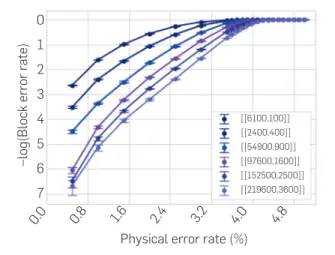
is due to the very crude bounds that we obtain via percolation theory arguments. In this work, we have not tried to optimize the value of the threshold and have instead tried to simplify the general scheme as much as possible. As shown in Figure 3, numerical simulations13 suggest nevertheless that the
thresh-old value for expander codes could be comparable to the best constructions based on concatenating surface codes.
Another limitation is in the geometry of quantum expander codes. Measuring the syndrome is simple in the sense that one needs to act on a small number of qubits, but the qubits will in general not be geometrically local. Performing gates that are not geometrically local may be significantly harder than nearest neighbor gates for many noiseless syndrome case described in the previous section.
The main difference is that we use the syndrome adjacency
graph of the code, which is similar to the adjacency graph
except that we also include check nodes as vertices. This is in order to ensure the “locality” of the decoding algorithm with respect to this graph, implying that each cluster of the error is corrected independently of the other ones. Using the fact that clusters are of size bounded by , the result on low weight errors shows that the size of is controlled by the syndrome error size. In order to show that the error after correction is local stochastic, a more delicate analy-sis is needed. For this, we introduce the notion of witness to assign residual qubit errors to neighboring syndrome errors. We refer to Fawzi et al.4 for details.
3.2. Parallelizing small-set-flip
We established that at each step of Algorithm 2.4, there are many possible flips F that decrease the syndrome weight. We already exploited this property to handle a noisy syndrome, but it can also be used to parallelize the decoding algorithm. In fact, we can now flip several of these small sets F
simulta-neously. However, we have to pay attention to the fact that
the sets σX(F) could intersect. In order to avoid that, we intro-duce a coloring of the X-type generators: if g1 and g2 have the same color, then for any F1 ⊆ ΓX(g1) and F2 ⊆ ΓX(g2): σX(F1) ∩
σX(F2) = ∅. It is simple to show that the set CZ of all the X-type generators can be partitioned using a constant number χ of
color classes .
This leads to Algorithm 2 that is a parallelized version of Algorithm 1 where we flip all the small sets that decrease the syndrome weight sufficiently and that have the same color. Let us discuss the stopping condition for this par-allelized decoding algorithm. The natural stopping con-dition (which is not exactly the one used in Algorithm 2) here would be similar to the sequential version: when no more flips decrease the syndrome weight. As one can show that the syndrome weight decreases by a constant frac-tion at each step, the number of steps for this algorithm would be of order and O(log n) we obtain the same result as in Theorem 3: the residual error is local stochastic with parameter only depending on psynd and not on the size of the initial error. Instead, in Algorithm 2, we apply a fixed number of steps f0, where f0 is a well-chosen constant that depends on the degrees and expansion parameters of the expander graph. This allows the decoding algorithm to run in constant time, which is important for fault tolerance if we do not assume that classical computations are instan-taneous. But the price to pay is that the residual error will not only depend on syndrome error rate psynd but also on the qubit error rate pphys. In particular, even if the syndrome was perfect, this algorithm would only reduce the size of the error but not completely correct it. This is however good enough in the context of fault tolerance. We refer the reader to Grospellier12 for more details.
Algorithm 2: Parallel small-set-flip decoding algorithm. INPUT: a syndrome where with an error on qubits and an error on the syndrome
research highlights
Omar Fawzi ([email protected]), Univ Lyon, ENS de Lyon, CNRS, UCBL, LIP Lyon, France.
Antoine Grospellier and Anthony Leverrier ({antoine.grospellier, anthony. [email protected]}@inria.fr), Inria, Paris, France.
quantum computing architectures. Note that this is in con-trast to the surface code for which the syndrome bits can be obtained by performing an operation on four neighbor-ing qubits on a two-dimensional lattice. One interestneighbor-ing (architecture-dependent) question for future research is to quantify to which extent a gain in the encoding rate jus-tifies the additional difficulty to perform gates that are not geometrically local.
A third limitation is that for our analysis to apply, we need bipartite expander graphs with a large (vertex) expansion. One issue is that there is no known efficient algorithm that can deterministically construct such graphs. Although algo-rithms to construct graphs with large spectral expansion are known, they do not imply a sufficient vertex expansion for our purpose. Random graphs will display the right expan-sion (provided their degree is large enough) with high prob-ability, and it is not known how to check efficiently that a given graph is indeed sufficiently expanding.
ACKNOWLEDGMENTS
We would like to thank Benjamin Audoux, Alain Couvreur, Anirudh Krishna, Vivien Londe, Jean-Pierre Tillich, and Gilles Zémor for many fruitful discussions on quantum codes as well as thank Gottesman for answering questions about his paper.11 OF acknowledges support from the ANR
through the project ACOM. AG and AL acknowledge support from the ANR through the QuantERA project QCDA.
quantum computation. Phys. Rev. A 3,
86 (2012), 032324.
7. Freedman, M.H., Meyer, D.A., Luo, F. Z2-systolic freedom and quantum codes. Mathematics of Quantum Computation. Chapman & Hall/CRC,
2002, 287–320.
8. Gallager, R. Low-density parity-check codes. IRE Trans. Inform. Theor. 1, 8
(1962), 21–28.
9. Gidney, C., Ekerå, M. How to factor 2048 bit RSA integers in 8 hours using 20 million noisy qubits. arXiv preprint arXiv:1905.09749 (2019).
10. Gottesman, D. Stabilizer codes and quantum error correction. PhD thesis,
California Institute of Technology (1997). 11. Gottesman, D. Fault-tolerant
quantum computation with constant overhead. Quant. Inform. Comput. 15–16, 14 (2014), 1338–1372.
12. Grospellier, A. Constant time decoding of quantum expander codes and application to fault-tolerant quantum computation. PhD thesis,
Inria Paris (2019).
13. Grouès, L., Grospellier, A., Krishna, A., Leverrier, A. Combining hard and soft decoding for hypergraph product codes. arXiv preprint arXiv:2004.11199 (2020). 14. Kovalev, A.A., Pryadko, L.P. Fault
tolerance of quantum low-density parity check codes with sublinear distance scaling. Phys. Rev. A 2, 87
(2013), 020304.
15. Leverrier, A., Tillich, J.-P., Zémor, G. Quantum expander codes. In
Proceedings of the 2015 IEEE 56th Annual Symposium on Foundations of Computer Science (FOCS) (2015),
IEEE, 810–824.
16. Pippenger, N. On networks of noisy gates. In Proceedings of the 26th Annual Symposium on Foundations of Computer Science
(SFCS 1985) (1985), IEEE, 30–38.
17. Pippenger, N., Stamoulis, G.D., Tsitsiklis, J.N. On a lower bound for the redundancy of reliable networks with noisy gates. IEEE Trans. Inform. Theory 3, 37 (1991), 639–643.
18. Shannon, C.E. A mathematical theory of communication. Bell Syst. Tech. J. 3, 27 (1948), 379–423.
19. Shor, P.W. Algorithms for quantum computation: Discrete logarithms and factoring. In Proceedings 35th Annual Symposium on Foundations of Computer Science (1994), IEEE,
124–134.
20. Shor, P.W. Scheme for reducing decoherence in quantum computer memory. Phys. Rev. A 4, 52 (1995),
R2493.
21. Shor, P.W. Fault-tolerant quantum computation. In Proceedings of 37th Conference on Foundations of Computer Science (1996), IEEE, 56–65.
22. Sipser, M., Spielman, D.A. Expander codes. IEEE Trans. Inform. Theory 6,
42 (1996), 1710–1722.
23. Steane, A.M. Error correcting codes in quantum theory. Phys. Rev. Lett. 5, 77
(1996), 793.
24. Tillich, J.-P., Zémor, G. Quantum LDPC codes with positive rate and minimum distance proportional to the square root of the blocklength. IEEE Trans. Inform. Theory 2, 60 (2014), 1193–1202.
25. Von Neumann, J. Probabilistic logics and the synthesis of reliable organisms from unreliable components. Autom. Stud., 34 (1956), 43–98.
Copyright held by authors/owners. Publication rights licensed to ACM. References
1. Aharonov, D., Ben-Or, M. Fault-tolerant quantum computation with constant error rate. SIAM J. Comput. 4, 38 (2008), 1207–1282.
2. Bombín, H. Single-shot fault-tolerant quantum error correction. Phys. Rev. X 3, 5 (2015), 031043.
3. Calderbank, A.R., Shor, P.W. Good quantum error-correcting codes exist.
Phys. Rev. A 2, 54 (1996), 1098.
4. Fawzi, O., Grospellier, A., Leverrier, A. Constant overhead quantum fault-tolerance with quantum
expander codes. In Proceedings of the 2018 IEEE 59th Annual Symposium on Foundations of Computer Science (FOCS) (2018),
IEEE, 743–754.
5. Fawzi, O., Grospellier, A., Leverrier, A. Efficient decoding of random errors for quantum expander codes. In
Proceedings of the 50th Annual ACM SIGACT Symposium on Theory of Computing (2018), ACM, 521–534.
6. Fowler, A.G., Mariantoni, M., Martinis, J.M., Cleland, A.N. Surface codes: Towards practical large-scale 0 1 2 3 4 5 6 7
Physical error rate (%) [[6100,100]] [[2400,400]] [[54900,900]] [[97600,1600]] [[152500,2500]] [[219600,3600]]
–log(Block error rate)
0.0 0.8 1.6 2.4 3.2 4.0 4.8
Figure 3. Logical error rates after decoding quantum hypergraph product codes of various blocklengths with the small-set-flip algorithm, as a function of the physical error rate for i.i.d. X-Pauli errors. These simulations were done with perfect syndrome (figure from Grouès et al.13).