Data science and advanced analytics : an integrated framework for creating value from data

Data Science and Advanced Analytics: An

integrated framework for creating value from data

by

Miguel Paredes

S.M., Massachusetts Institute of Technology (2008)

M.C.P., Massachusetts Institute of Technology (2008)

Submitted to the Interdisciplinary PhD Committee in Data Science &

Department of Urban Studies and Planning

in partial fulfillment of the requirements for the degree of

Doctor of Philosophy in Data Science

at the

MASSACHUSETTS INSTITUTE OF TECHNOLOGY

September 2018

@

Miguel Paredes, MMXVIII. All rights reserved.

The author hereby grants to MIT permission to reproduce and to

distribute publicly paper and electronic copies of this thesis document

in whole or in part in any medium now known or hereafter created.

Signature of Author .

Signature redacted

Interdisciplinary

in4ta Science & Department of Urban Studies

and Planning

Certified by...

Signature redacted

June 22, 2018

V

_{Una-May O'Reilly}

Principal Research Scientist, Computer Science and Artificial

Intelligence Lab

A ccepted by ...

Accepted

PhD

Thesis Co-Supervisor

Signature redacted

67

Roy Welsch

Chair, Interdisciplinary PhD Committee in Data Science

.Signature

redacted

Thesis Co-Supervisor

-b y .... ... :> U

Lawrence Vale Committee Chair, Department of Urban Studies and Planning

Data Science and Advanced Analytics: An integrated

framework for creating value from data

by

Miguel Paredes

Submitted to the Interdisciplinary PhD Committee in Data Science & Department of Urban Studies and Planning

on August 23, 2018, in partial fulfillment of the requirements for the degree of

Doctor of Philosophy in Data Science

Abstract

Fundamental problems in society, such as medical decision support, urban planning and customer management, can be addressed by data-driven modeling. Frequently, the only data available are observational rather than experimental. This precludes causal inference, though it supports quasi-causal inference (or causal approximation) and prediction. With three different studies that are driven by observational data, this thesis compares machine learning and econometric modeling in terms of their purposes, insights, and uses. It proposes a data science methodology that combines both types of modeling to enable experimental designs which would otherwise be impossible to carry out. In the first two studies, we address problems through both a prediction and quasi-causation approach (i.e. machine learning and econometrics), exploring their similarities, differences, benefits, and limitations. These two initial studies serve to demonstrate the need for an end-to-end methodology that combines prediction and causation. Our proposed data science methodology is presented in the third study, in which an enterprise seeks to address its customer churn. First, it uses observational data and econometrics to approximate the causal determinants of churn (quasi-causal insights). Second, it uses machine learning to predict churn likelihoods of clients, and selects a study group with likelihoods above a threshold of interest. Third, the quasi-causal insights are used to design a stratified randomized controlled trial (i.e. A/B test) where study subjects are randomly assigned to one of three experimental groups. Finally, thanks to the rigorously designed experiment, the causal effects of the interventions are determined, and the cost-effectiveness of

the treatments relative to the control group are established. Thesis Co-Supervisor: Una-May O'Reilly

Acknowledgments

I would like to thank God for always being there and giving more than I deserve. I

would like to thank my wife, whose support made this PhD possible. I would like to thank my daughters, whom ground me and remind me of what is important in life. I would like to thank my parents, whose hard work, love, and example allowed me to be where I am today. I want to thank Una-May O'Reilly, for being such an amazing adviser and human being, and who believed in me. I want to thank Roy Welsch, who stood by me during struggles in the PhD. I want to thank David Geltner, whose kindness and generosity are only matched by his intellectual brilliance. I especially want to thank Dean Blanche Statton, Larry Vale, and Amy Glassmeir; this PhD is in existence only because of you three. I especially want to thank Erik Hemberg for being so generous with his time and "whiping" me into finishing the work needed for this dissertation. I want to thank MIT, for being the best place on earth. I want to thank my friends, to whom I have not been a friend in so long. Finally, I want to thank Breca, for allowing me to put in practice what I have learned througought this PhD, and for wanting to transform Peru through Al, Data Science, and Advanced Analytics and giving me the honor of helping lead these efforts.

Bibliography 1 Introduction

1.1 The need for an integrative Data Science methodology 1.2 Methodological Framework . . . .

Research Questions . . . . H ypothesis . . . . M ethods . . . .

1.5.1 Quasi-causation through Econometrics

1.5.2 Prediction through Machine Learning

1.5.3 Causation through Experimental Design

1.6 Organization

2 On the Challenges of using Propensity Intensive Care Unit patients

2.1 Introduction . . . . 2.2 M ethods . . . . 2.3 Experiments . . . . 2.3.1 D ata . . . . 2.3.2 Setup . . . . 2.3.3 Post-Matching Balance . . . . 2.4 Results and Discussion . . . .

Score Matching to study 22 22 24 25 25 27 28 28

Contents

9 1.3 1.4 1.5 10 12 13 14 15 16 16 17 18 20

3 Machine Learning or Discrete Choice Models for Car Ownership

Demand Estimation and Prediction? 34

3.1 Introduction . . . . 34

3.2 Data .. ... 37

3.2.1 HITS 2012 Insights ... ... 38

3.3 Methods ... ... 38

3.3.1 Discrete Choice Models . . . . 39

3.3.2 Machine Learning Models . . . . 39

3.4 Experim ents . . . . 40

3.4.1 Data Preparation . . . . 40

3.4.2 Setup . . . . 42

3.5 R esults . . . . 43

3.5.1 Prediction from EDC . . . . . . .. .. . . . . . . . . .. 43

3.5.2 Prediction Using EML . . . . . . . . .. . . . . 45

3.6 Conclusion & Future Work . . . . 46

4 A Case Study on Reducing Auto Insurance Attrition with Econo-metrics, Machine Learning, and A/B testing 50 4.1 Introduction . . . . 50

4.2 D ata .. . . . ... . . . .. .. . . . . . 52

4.2.1 Auto insurance in a latin american country . . . . 52

4.2.2 Data cleaning, preparation, and final dataset . . . . 52

4.3 M ethods . . . . 53

4.3.1 Econom etrics . . . . 54

4.3.2 M achine Learning . . . . 54

4.3.3 Experimental Design . . . . 55

4.4 Experim ents . . . . 56

4.4.1 Quasi-Causation through Econometrics . . . . 56

4.4.3 Causation through A/B Testing . . . . 58

4.5 R esults . . . . 58

4.6 Conclusions, Limitations and Future Work . . . . 61

5 Conclusion and Discussion 63

A Tables 66

B Figures 75

List of Figures

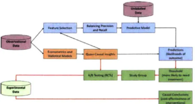
1-1 Data Science and Advanced Analytics Methodology

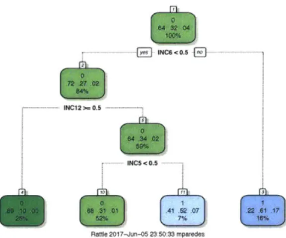
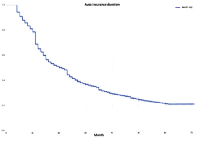
3-1 Decision tree model . . . . 4-1 Survival Analysis curve . . . . 4-2 Survival Regression curve by Age Group . . . .

5-1 Data Science and Advanced Analytics Methodology .

B-1 Decision tree model . . . . B-2 Survival Analysis curve . . . . B-3 Survival Regression curve by Age Group . . . .

11 44 59 60 64 75 76 77

List of Tables

2.1 MIMIC dataset extraction and filtering steps . . . . 26

2.2 Patient Features . . . . 27

2.3 Cohort Balance between D+ and D patients. Summary of average feature values. Systematic differences between D+ and D- patients . 31 2.4 R esults . . . . 32

2.5 Post Matching Cohort Balance between D+ and D- patients. Feature Balance between D+ and D- patients . . . . 33

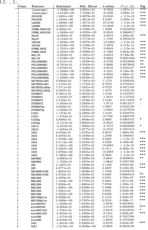
3.1 Coefficients of MNL on EDC. Signif. codes are 0:***, 0.001:**, 0.01:*, 0.05:., 0.1: , 1:. . . . . 47

3.2 Discrete Choice vs. Machine Learning model Prediction Accuracy re-sults on EMNL . . . . . . . . .. . . . . . ..48

3.3 Machine Learning model Prediction Accuracy results on EML . . . . 49

4.1 Different Machine Learning Models Performance . . . . 60

4.2 Randomized Control Trial Results . . . . 60

A.1 MIMIC dataset extraction and filtering steps . . . . 66

A .2 Patient Features . . . . 67

A.3 Cohort Balance between D+ and D- patients. Summary of average feature values. Systematic differences between D+ and D- patients . 68 A .4 R esults . . . . 69

A.5 Post Matching Cohort Balance between D+ and D- patients. Feature Balance between D+ and D- patients . . . . 70

A.6 Coefficients of MNL on EDC. Signif. codes are 0:***, 0.001:**, 0.01:*,

0.05:., 0 .1: , 1:. . . . . 71

A.7 Discrete Choice vs. Machine Learning model Prediction Accuracy

re-sults on EMNL . . . . . -. -. . - -. . - -. - - - .72

-A.8 Machine Learning model Prediction Accuracy results on EML . .- . 73 A.9 Different Machine Learning Models Performance . . . . 74

Chapter 1

Introduction

There are fundamental problems in society that can better be addressed by build-ing analytical models that leverage data. For example, the results from analytical models applied to appropriate data can help doctors make better decisions in the

ICU, help planners and engineers better design and build cities, and help

compa-nies better understand why their customers are switching to competitors. In most cases, these available data are observational (i.e. the researcher has no control over how the data is generated), and not experimental (i.e. the researcher designs the data generating conditions and setting). Observational data can be used for predic-tion (i.e. forecasting what will occur next) and quasi-causapredic-tion (i.e. understanding what is occurring and approximating the causes why) [3, 39], but bias in the data precludes causation (i.e. causal inference, or determining the cause) [30]. Machine learning models are optimized for prediction from observational data [2,12,25], while econometric and statistical models are optimized for quasi-causation from observa-tional data (i.e. for explaining the association or relationship between input and outcome variables and approximating, but not establishing, causal effects and rela-tionships) [19,30]. However, econometric and statistical models are also employed for prediction, conditional on certain modeling constraints, such as only subscribing to certain classes of functions (e.g. linear models), or non-algorithmic feature and model selection mechanisms [3,49].

Figure 1-1: Data Science and Advanced Analytics Methodology

from different disciplines and applies them to observational and experimental data to support decision making. Figure 1 summarizes our work. While much work has been and is done on either prediction or quasi-causation using observational data (upper part of the diagram), we argue that both can be employed jointly and show how this can be done. Furthermore, we demonstrate how prediction can bu used to indicate who should be recruited into a study group to produce experimental data necessary to establish causality (red line feeding into A/B testing, which allows for causation), which tends to be elusive in analytical studies.

We present three case studies where we apply our data science and advanced an-alytics methodology to observational data to address quasi-causation or prediction problems. In all case studies, we develop econometric or statistical models to un-derstand a problem and approximate its causes, and we construct machine learning models to predict and anticipate the problem in the future. In our third case study we demonstrate the value of generating and collecting experimental data, which allows us to establish causation. More importantly, our specific contribution is demonstrating how quasi-causation through econometrics and prediction through machine learning can enable, through A/B testing, establishing a causal relationship between an inter-vention and outcome of interest.

1.1

The need for an integrative Data Science

method-ology

People, institutions, and organizations are used to making decisions under conditions of uncertainty. The process through which decisions are made can vary depending on the degree of certainty of the outcome. For example, doctors face many decisions for which clinical trials are lacking, thus they make decisions based on their best predictions, which are informed by experience, similar studies, colleague consultation, etc. Sometimes doctors can make a more informed decision based on observational studies which try to approximate causal evidence (we shall call these quasi-causality). Furthermore, sometimes doctors face medical choices for which clinical trials exist and protocols have been established, thus basing their decisions on actual causal evidence. Data science has gained popularity in the last decade due to a proliferation of data [35,421, and decrease in computational and storage costs

[36,45].

However, data science solutions have not always taken advantage of methods from all its underlying fields, such as econometrics, statistics, machine learning, or experimental design, but rather address problems using methods from individual fields. There are two main reasons for this. First, there has been a lack of interdisciplinary work between fields such as econometrics and machine learning, which has prevented cross-fertilization [4, 40, 51]. Second, the objectives of different fields, and therefore of their methods, are different. For example, machine learning methods are designed and optimized for predicting a system's outcomes, while econometric and statistical models are designed and optimized for approximating the causal mechanisms of a system [40,52]. We argue that data science can be more powerful and effective when it takes advantage of a breadth of methods. However, in doing this, one needs to reconcile the premises of different methods and chape their complementarity. This thesis provides a roadmap on how this can be done.

1.2

Methodological Framework

Our main contribution is presenting a data science and advanced analytics method-ology that is comprehensive in the data and methods it can leverage. Our specific contributions are two: 1) integrating methods from typically disjoint fields (economet-rics and machine learning) to more effectively perform prediction and quasi-causation, and 2) proposing a method through which we use econometrics and machine learning to design a less expensive, more informative controlled statistical experimenta based on causality (prediction enabling causation). We present several examples of how to partially or fully apply our methodology. Our first application is in healthcare, where we employ econometrics and statistical modeling on observational data from inten-sive care units (ICUs) to approximate the causal effects of administering diuretics to sepsis patients (i.e. quasi-causality). An important problem with observational studies is dealing with biased and confounded data [19]. A typical approach is to use econometric and statistical models to control for systematic differences in the observ-able space

[6,

30]. Under certain assumptions and conditions, one can approximate

the effect of an intervention by making appropriate comparisons of patients [5,6,44]. For example, one can match patients on their estimated probability of diuretics treat-ment. In other words, one can compare patients with similar severity of sepsis with and without diuretics treatment.

Our second application contrasts machine learning to statistical modeling and econometrics on the prediction task in the urban transportation space. Using survey data from Singapore in year 2008 we try to understand the determinants of household car ownership, and then predict household car ownership in 2012. We demonstrate that predictions from machine learning are superior to those of econometrics or statis-tical models, because machine learning is not constrained to the use of linear models (needed for interpretability and thus used extensively in the latter models), its model and feature selection process is algorithmic rather than manual (thus covering a larger model and feature space), and it tests the prediction of its many different models on hold-out data (i.e. test data) [2,4,12,25].

Finally, our third application is in the insurance space where we use econometrics, machine learning, and experimental design together to help a leading Latin American insurance company reduce customer attrition. We estimate a discrete choice model for a customer's decision to renew their auto insurance policy, and a survival regression model to estimate the policy's duration [9,38,49]. From these models we learn which variables are most associated with churn, which we will use to inform our predictive model and to design our randomized control trial. Next, we use machine learning models to predict which customers will churn in the next three months, using the quasi-causal insights from our econometric models to inform and complement tradi-tional model selection and feature selection. Finally, based on the ranked likelihood of a client to churn, we select those with probability higher than 0.7, design an exper-imental design (i.e. A/B test) where we randomly assignment to three experexper-imental groups (control, treatment A, and treatment B) and test the cost-effectiveness of two different churn-reducing interventions. We uncover causal effects thanks to the rig-orous experimental design, and show that the most cost-effective intervention helped the insurance company reduce churn in 6 percentage points, which after a year will accrue to US$750,000 of additional revenues.

In this thesis we show that while econometrics and machine learning are con-structed for different objectives (quasi-causation or causation vs. prediction), op-portunities for cross-fertilization exist. Furthermore, we show how causation and prediction can be addressed simultaneously, and how prediction can enable causa-tion.

1.3

Research Questions

In each piece of presented work, we are motivated by the following four questions. First, we want to understand, as much as the data allows, what is happening in the system being studied (description). Second, we want to hypothesize why the observed outcome is occurring. In most cases, we will not be able to establish causality but rather obtain quasi-causality insights (quasi-causality). Third, we want to understand

the system's future outcome (prediction). Finally, we will want to do something to the system when the predictions are unfavorable and understand how effective our intervention(s) is at changing the system's outcome.

Additionally, we have the following secondary research questions:, which are ex-plored in the three papers:

* What type of decision-making problems are better addressed through prediction or through causation?

" Why are the results of prediction models different from those of causal models

when the latter are representation of the system?

" How can machine learning models improve the quality of conclusions drawn

from observational studies and the approximation of causal inference?

" How can prediction models be exploited to develop causal studies that lead to

causation models?

1.4

Hypothesis

Our first hypothesis is that in the absence of a causal model, quasi-casual and pre-diction models will suffice. We test this hypothesis in the context of Intensive Care Unit (ICU) clinical data of patients diagnosed with sepsis, for which a clinical trial uncovering the causal effect of administering diuretics is lacking.

Our second hypothesis is that prediction models (e.g. machine learning models) will outperform quasi-causal models (e.g. econometric or statistical models) on the prediction task. We test this hypothesis on 2008 and 2012 survey data from Singa-pore where we compare prediction and quasi-causal models on predicting whether a household will own one (or more) vehicles or not.

Finally, our third hypothesis is that an experimental setting that supports es-tablishing causality can be prepared through the combined use of econometrics and machine learning. We test this in the context of one of Latin America's largest

in-econometrics, then predict which clients will churn in the next three months, and finally run a randomized control trial on a study group of clients with a higher-than

70% chance of churning, stratifying the randomization based on the determinants

previously identified.

1.5

Methods

Our data science and advanced analytics framework consist of methods from three main disciplines: econometrics, machine learning, and experimental design. These methods are used in the three case studies and are described below.

1.5.1

Quasi-causation through Econometrics

Econometrics is a branch of economics that focuses on the use of mathematical and statistical models to describe economic systems and the relationships of their subsys-tems

[3].

A core aspect of econometrics is regression analysis, which seeks to explain

a dependent variable Y using a vector of explanatory or independent variables X. For example, as in this case study, modeling the relationship between customer churn (dependent variable) and a series of variables that might affect or explain churn (inde-pendent variables), such as a customer's age, income, labor status, distance to work, etc.

There are many types of regression models besides the linear regression model

[3]. In this paper we employ a discrete choice regression model (logit) to model

a customer's choice to continue or not with their auto insurance, and a survival regression to model a customer's policy tenure or duration [9], [101, [26].

The traditional setup for an econometric model relating Y to a transposed vector of features X' is Y - Xj = ej, where ej is the stochastic or error term, which represents

things such as omitted variable bias, measurement errors, differences in the functional form, and pure randomness in human behavior. This is usually done by minimizing the sum of squared residuals.

or parameters /3 in such a way that the model represents the data as accurately as possible. In other words, econometrics seeks to minimize estimation error

(0

- 3), to obtain unbiased estimators, and to do so it requires as much information as possible, which is why estimation is usually done with most, if not all, of the data.

= o + 3₁Xi + i (1.1)

An important aspect of econometrics, in contrast with machine learning, is that one believes there is a model governing the data generating process, the formula or model specification, and that this model can and should be approximated as closely to reality as possible. In other words, econometrics is guided by a theory of the world, and its main objective it to describe, and possibly explain, the phenomena at hand as accurately as possible. In this sense, econometrics, for the most part, is a representation of Leo Breiman's description of the data model statistical culture [14].

Another important aspect of many econometric models, especially regression mod-els, is that they are linear in the parameters' to be more easily interpretable. For example, in our model (1), one-unit increase in X1 would represent an increase of Betal in Y. This is important because coefficients have a direct interpretation of as-sociation ceteris paribus which people can understand. Finally, while prediction is common in econometrics, it is secondary and conditional to this best-approximated model. In other words, predictions are made based on the estimated model, which is optimized for explanation or description, but not optimized for prediction, unlike machine learning.

1.5.2

Prediction through Machine Learning

The focus of machine learning is to support making decisions or predictions based on data. Machine learning is an interdisciplinary field with strong roots in com-puter science, statistics, information science, and others [21, [12]. There are many different types of machine learning (e.g. supervised learning, unsupervised learning, semi-supervised learning, reinforcement learning, deep learning), but this case study

will focus on supervised learning algorithms. A supervised learning algorithm takes training data D in the form of a set of pairs {(x1, yi), (X2, Y2), AAe, (x., y.)} where xi

are properties or attributes of an entity to be classified or predicted, being represented

by a D-dimensional vector of real and/or discrete values usually called features, and yi is an element of discrete or continuous values called labels. The objective of a

supervised machine learning algorithm is, given a new input value xi+1, to correctly

classify or predict the value of yi+1. Different supervised machine learning algorithms approach the prediction problem differently, but all of them "learn" from data given to them in a process called training, where the algorithms are given labels along with their corresponding features to find the patterns governing the relationship between features and labels. After a model has been learned, features from data the model has not seen (test or validation datasets) are given to the model and the predictions are compared to the ground truth (the labels from the test or validation sets that were not seen by the algorithm). Models can then be evaluated on different performance measures (e.g. accuracy, recall, precision, AUC, etc.). In contrast to econometrics, machine learning does not assume that a model governing the data generating process exists nor does it presume to be able nor does it want to be able to approximate it. In this sense, econometrics, for the most part, is a representation of Leo Breiman's description of the data model statistical culture [14].

While econometrics is interested in minimizing the estimation error, machine learning is interested in minimizing the prediction error (y - y). Machine learning

tries to extract as much information as it can from the training data in order to be able to generalize and predict future data points. Therefore, the models that machine learning employs are not constrained to interpretability nor linearity in the parameters.

1.5.3

Causation through Experimental Design

The main idea behind experimental design, a branch of statistics with applications in many fields, is to design interventions that can be assessed rigorously in controlled environments [24]. Experimental design is present in many fields and takes different

names. In the medical field it is called clinical trials

130].

In economics and the social sciences, it is called randomized controlled trials [22], [271, 128]. More recently, in the online and digital world, it is called A/B testing [181.

Experimental designs are employed when one wants to be able to have a high degree of certainty regarding the causal effect of an intervention, or to assess the cost-effectiveness of different competing interventions. For example, in our auto in-surance case, we designed an experiment to evaluate the causal effects of two different churn retention campaigns. Experimental designs tackle the fundamental problem of causal inference, which has to do with the fact that we either observe the world with or without an intervention, thus preventing us from comparing both states. In other words, we never observe the counterfactual [28],

[30],

[39] but only the factual

outcome. In the absense of experimentation, this observed outcome presents bias (e.g. churning clients have systematic similarities) and confounding (e.g. there are unobservable variables which are driving churn), which precludes reliable causation. When experimentation is not an option, an approach taken by social scientists is to run quasi-experimental analysis over observational data, although these types of studies usually do not allow for inferring causality except under certain assumptions or circumstances and are prey to selection bias

[19].

Different approaches for studying causality exist in different disciplines. For ex-ample, Judea Pearl's do-calculus and causality framework in computer science, or the Neyman-Rubin causal model (also called the Potential Outcomes Model) from statistics and econometrics [28,41].

The main idea behind experimental design, a branch of statistics with applications in many fields, is to design interventions that can be assessed rigorously in controlled environments

[24].

Experimental designs tackle the fundamental problem of causal inference, which has to do with the fact that we either observe the world with or with-out an intervention, thus preventing us from comparing both states. In other words, we never observe the counterfactual [28], [30], [39] but only the factual outcome. In the absense of experimentation, this observed outcome presents bias (e.g. churning clients have systematic similarities) and confounding (e.g. there are unobservable

variables which are driving churn), which precludes reliable causation.

To design and run an experiment, as we do in this case study, one needs the following:

e A population where one wants to intervene and effect. e A minimum sample size (n).

e One or more interventions whose effect we want to assess.

e To define the parameters for statistical significance (usually 95%) and statistical

power (usually 80%)

9 A randomization mechanism (pure, stratified, etc.), and the variables to stratify

if not a simple randomization.

e A minimal detectable effect size (MDE).

With these parameters, one can design an experiment to assess the causal effect of the interventions. While econometrics traditionally uses observational data, and must rely on quasi-experiments to approximate causal effects, randomized experiments employ experimental data produced by a researcher or organization. For a few good resources and guides to perform the power calculations and design the randomized experiments see [13, 22, 27, 30].

1.6

Organization

This dissertation follows a three-paper approach, in which I discuss applications in three fields. These three journal papers have been or are in the process of being peer-reviewed. The first was presented at the NIPS 2016 Healthcare Workshop in December 2016. The second appeared in the IEEE Advances in Models for Trans-portation Research in June 2017. Finally, the third paper has been submitted for consideration for presentation and publication in the 2018 IEEE Data Science and Advanced Analytics conference and proceedings.

The rest of this thesis is organized around the three papers. Chapter 2 (On the Challenges of using Propensity Score Matching to study Intensive Care Unit pa-tients) employs observational data from US ICU units, develops econometric models to approximate the causal effect of administering diuretics to sepsis patients (quasi-causation), and uses machine learning to predict patient mortality and ICU length of stay. Chapter 3 (Machine Learning or Discrete Choice Models for Car Ownership De-mand Estimation and Prediction?) uses observational data to estimate discrete choice econometric models of household car ownership in 2008, and then predict household ownership in 2012. We then train a machine learning model on the same 2008 sur-vey data, and predict 2012 household car ownership. We compare the predictions of econometrics and machine learning and conclude that the latter is better suited for in-creased prediction accuracy, and explain why. Chapter 4 (A Case Study on Reducing Auto Insurance Attrition with Econometrics, Machine Learning, and A/B testing). Chapter 5 presents the thesis conclusions and discusses assumptions, limitations, and future work.

Chapter 2

On the Challenges of using

Propensity Score Matching to study

Intensive Care Unit patients

2.1

Introduction

Uncertainty is inherent to most Intensive Care Unit (ICU) decisions. Physicians must make critical choices in the ICU without complete and explicit knowledge of a treatment's causal mechanisms and its efficacy. For example, physicians must choose whether to administer diuretics to patients with a sepsis diagnosis when the treatment has not been investigated with a clinical trial.

Data on patients' health are constantly being measured in the ICU, enabling observational studies. These studies try to approximate the causal effects that clin-ical trials would provide by comparing the outcome of interest (e.g. mortality) be-tween the group of patients who received an intervention (the treatment group) and a group of patients who did not receive a treatment (the control group) but who are very similar in terms of relevant health status indicators (i.e. features). Propensity Score Matching (PSM), a very common observational study approach, calculates a similarity-of-treatment score for every patient (treatment or control) based on their

features, and then matches patients on this score

[44].

Although popular, PSM does not lack its skeptics and deterrents, credibly arguing that in prospective studies such as PSM discrepancies beyond chance do occur and differences in estimated magni-tude of treatment effects are very common [31]. Additional authors maintain that

PS methods are inconsistently and poorly applied [5,8]. Austin analyzes 47 articles

published between 1996 and 2003 in the medical literature that employed PSM with varying results

[8].

After reviewing PSM health articles from the last decade the same author claims that a frequently overlooked aspects is whether the PSM has been ad-equately specified

17].

The mixed findings from this body of literature motivated the efforts in this paper to experimentally apply PS methods to a specific clinical study using some relatively recent variants of PS methods in an effort to appraise their value [211.

Our study uses the MIMIC II critical care database [33] to explore the effect of diuretics administration on patients with a sepsis diagnosis through an observational study that matches diuretics positive patients (D+) to diuretics negative patients (D-). Before matching, we observe that D+ and D- patients experience the same mortality rates, and that D+ patients spend 8.8 additional days in the ICU. However, because we observe significant health differences between (D+) and (D+-) patients on a number of features upon entrance to the ICU, we apply PSM to control for these differences [20]. Given that PSM is highly parameterized we investigate the suitability and effectiveness of employing the method in this context, with the goal of explaining why or why not. Our approach is to run multiple experiments of various models to evaluate and compare their results.

We proceed as follows; Section 2 describes PSM and the parameters that must be selected to run the study. Section 3 describes the data, lays out our experimental setup, and presents the post-matching balance. Section 4 presents the results and provides a discussion. Finally, we suggest future work.

2.2

Methods

We use Propensity Score Matching (PSM), which builds a similarity-of-treatment score (i.e. the propensity score or PS) from a set of patient features (D+ and D-) and then matches patients on this score. A PS is the conditional probability of assignment to a particular treatment given a vector of observed covariates. In our model, the study group compares treatment (being administered diuretics) vs. no treatment (not receiving diuretics), denoted by the variable z with values 1 and 0. Each patient is represented by a set of covariates x = {1 i, X2, ..., X6 6}. The propensity score then is

the conditional probability that a patient with vector x of observed covariates will be assigned to treatment, given by:

e(x) = Pr(z = Ix). (2.1)

A PS can be estimated using a logit model for

e

eX

C(y)

= Z + Tf (X) (2.2) - e(y)

where y =log[

],

a and 0 are parameters, and

f(.)

defines a regression function.

66 covariates of the study group were included in the initial propensity score model.

Many propensity score models can be built depending on the vector of features de-fined and the model specification used. Given this ample design space, one common approach is to iteratively explore combination of features, selecting the combination that maximizes the gain of information on the outcome of interest. An important assumption in any PSM experiment is that the treatment selection mechanism is ig-norable; i.e., that all information needed to control for confoundness are contained in the features.

We develop several diuretics propensity models by running logistic regressions of the different feature sets on the diuretics indicator. We then use these models to obtain each patient's PS score, which can be interpreted as the probability that a particular patient will be administered diuretics, conditional on the selected health

indicators. After the PS is produced for each patient, we discard D- patients with minimal feature support (i.e. a score outside the range of D+ patient scores). For every D+ patient, we match them to at least one D-patient based on one of three similarity measures (Euclidean, Mahalanobis, and PS), and check for experimental group balance to assess the equivalence in health indicators. Finally, we estimate the average treatment effects on the treated (ATT), obtaining standard errors and p-values, by regressing the outcome variable (30 day mortality or length of stay) on either the PS, a set of feature, or a combination of both.

We use the dataset described in section 3.1 and choose the parameters we will vary. We select five health indicators sets (all features, best feature set defined through a stepwise algorithm, two sets of features suggested by physicians, and a set of features selected through a genetic algorithm [21]). We allow more than one D- patient to be matched to each D+ patient, allow matching with replacement (D- patients can be matched more than once), define a similarity measure (Euclidean, Mahalanobis, and PS), and select nearest neighbor as the matching algorithm. This combination of parameter definitions leads us to 9 different models for each outcome as seen in Table A.4.

2.3

Experiments

2.3.1

Data

We use the MIMIC II database, which contains patient records from intensive care units in Boston [331 and after data extraction and filtering obtain a study group of

1,522 patients (3.81% of the entire MIMIC database). Table A.1 shows the extraction

and filtering steps.

Of the 1,522 study group patients, 189 were D+ (12.4% of study group), and

1,333 (87.6% of study group) were D~. For each patient, age, gender, and race were obtained along with 21 clinical features as can be seen in table A.2. These 21 clinical features were measured on three days (day of entry, day before and day of diuretics

Table 2.1: MIMIC dataset extraction and filtering steps

Step Type Sample size %

All patients in MIMIC database 39,919 100%

1 All 3 IDs available 36,708 92.0%

2 Single hospital admission 26,027 65.2%

3 1+ day ICU data available 18,770 47.0%

4 Adult patients (remove neonates) 15,176 38.0%

5 Patients with sepsis diagnosis without Comfort Measures Only 1,644 4.1%

7 Discharge summary available 1,638 4.1%

8 Diuretics naive 1,606 4.0%

9 Filter for missing data 1,522 3.8%

decision) for a total of 66 features per patient. Additionally, there are two outcomes measures for each patient: 30 day mortality after ICU discharge, and ICU length of stay.

A fundamental problem to approximate the causal effects of diuretics on sepsis

patients is that patients arrive into the ICU with varying degrees of illness severity. This implies that there is no common timepoint after entering the ICU when the treatment decision is made. As well, there is no standard set of health indicator levels that determine if the patient should receive diuretics. There are different ways to normalize this temporal and severity difference. We use the median of the day of diuretics administration in the D+ group as the timepoint for when we reference D-patients. The median was day 4, and we filtered any D+ patients who were discharged or received diuretics before this day.

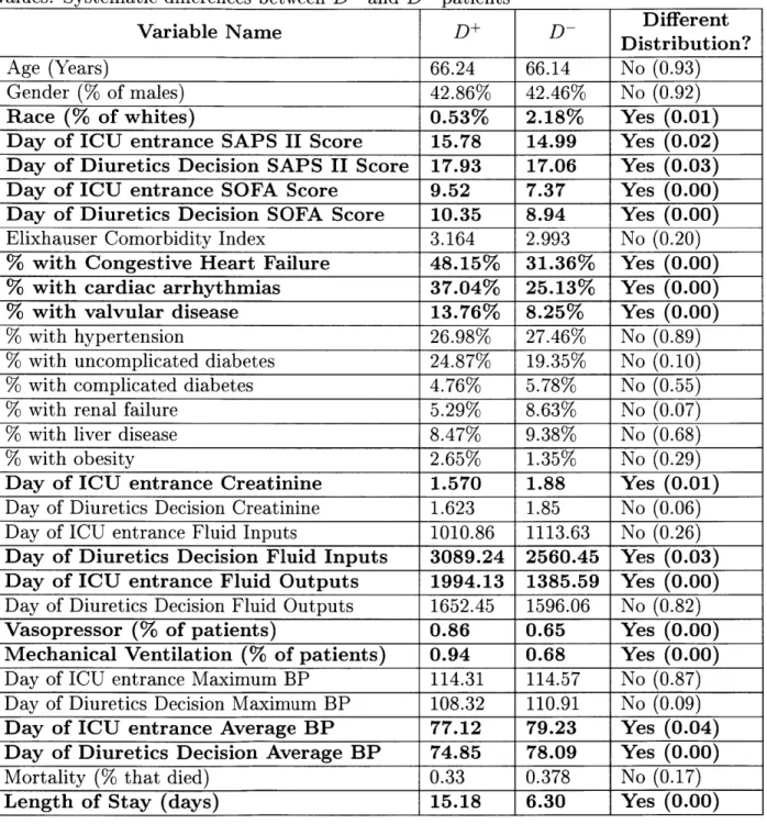
Table A.3 summarizes the average values for all clinical variables (with exception of measurements taken on day 1 and day 2) within each group for D+ and D- patients, and shows whether these mean differences are statistically different through a Welch two sample t-test.

From Table A.3 we can see that diuretics patients have significantly different health conditions upon entering the ICU (marked in boldface), and also at the moment when the decision to receive diuretics was taken. This suggests that we face selection bias. Patients who receive diuretics are more ill when they come into the ICU (higher SAPS II, SOFA scores), and on the diuretics decision day (SAPS II score, SOFA score). This

Table 2.2: Patient Features Age

Gender

Race (white

/

non-white)

SAPS II Score SOFA Score

Elixhauser Comorbidity Index Congestive Heart Failure Indicator Cardiac Arrhythmias Indicator Valvular Disease Indicator Hypertension Indicator

Uncomplicated Diabetes Indicator Complicated Diabetes Indicator Renal Failure Indicator

Liver Disease Indicator Obesity Indicator

Creatinine Level (day of measurement average) Fluid Inputs (day of measurement sum)

Fluid Outputs (day of measurment sum) Vasopressor Use

Mechanical Ventilation Use

Maximum Blood Pressure (on measurement day) Average BP (on measurement day)

Mortality (did patient die within 30 days of leaving ICU) Length of Stay (days)

worse health can be a confounding factor by influencing diuretics decision and health outcomes. Additionally, diuretics patients seem to have overall higher morbidity (congestive heart failure, cardiac arrythmia, and valvular disease). We also observe higher fluid levels, higher creatinine levels, and higher need for mechanical ventilation or vasopressors for D+ patients. We conclude from this analysis that a method that

addresses selection bias and confounding, such as PSM, is needed and appropriate.

2.3.2

Setup

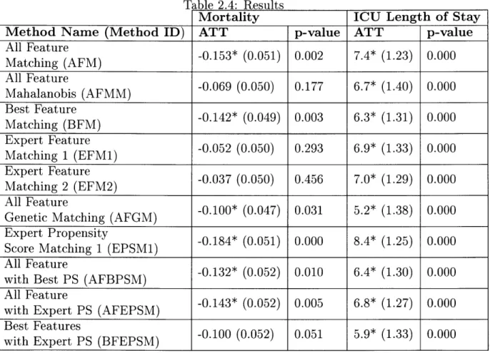
To estimate the Average Treatment Effects on the Treated (ATT) of diuretics on patients with a sepsis diagnosis, we run 9 different models for each of the two outcomes of interest. The experimental setup is reported in Table A.4.

The second and fourth columns show the average treatment effect on the treated (ATT) estimates for mortality and length of stay. A negative mortality value means that diuretics are associated with a percentage point reduction in mortality rates. The third and fifth columns present the p-values and the statistical significance of the ATT results (p-value < 0.05 is statistically significant at a = 0.05).

All methods match one D+ to one D patient, except model EPSM which uses 470 D- patients. The first five models only use a set of features but do not include a PS. Model BFM uses a forward

/

backward feature selection algorithm to select the best set of features that minimize the AIC of the diuretics logistic regression model [32]. Model AFGM employs a genetic algorithm to produce the optimal set of feature weights [21]. The EPSM1 model only uses a PS that was constructed from the 1st feature set provided by physicians. The final three models use either all features or the best subset of features and a PS score.

2.3.3

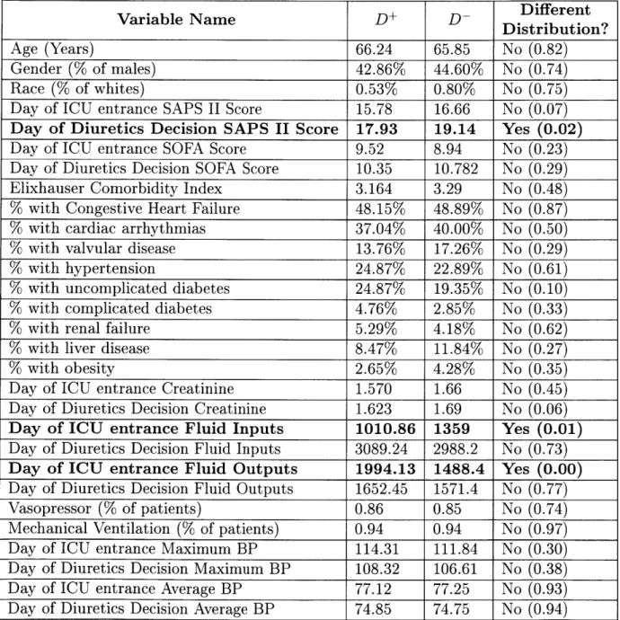
Post-Matching Balance

When using PSM methods to estimate ATTs, we must check for how balanced the treatment and control groups are after matching. In Table A.5 we present the post-matching feature balance for the EPSM1 model showing whether these mean differ-ences are statistically different through a Welch two sample t-test.

We can see that all features are now balanced except for SAPS II score for the day of diuretics decision, and the day of entrance for both the fluid inputs and outputs. Given that the measurement for input and output of fluids on the day of ICU entry are not balanced, this raises questions regarding this particular matching method's ability to control for observables.

2.4

Results and Discussion

We run 9 experiments for each outcome tuning different matching parameters, and find that diuretics is associated with a 10% (FGM model) to 18% (EPSM1 model) mortality decrease and between 5.9 (AFGM model) to 8.4 (EPSM1 model) additional

ICU days, suggesting that the effect of diuretics was being underestimated when com-paring these outcomes but not controling for confounding and selection bias through matching.

Recall we started out asking about the suitability and effectiveness of employing PSM in a critical care context, with the goal of explaining why or why not. Knowing that PSM is highly parametrized, we ran many experiments tuning these parameters. Our findings confirm what is known in the literature: that employing different feature sets and distance metrics impact the PS and the ATT obtained. For example, we found that out of the models that produced statistically significant treatment effects

EPSM1 was the only one that relied solely on the PS for matching.

These mixed results raise questions about how much researchers and practitioners can rely on insights obtained from applying PS methods to clinical data. Not knowing the underlying causal mechanism for treating septic patients appears to undermine even further the applicability of PSM.

As mentioned, a fundamental problem to approximate the causal effects of di-uretics on sepsis patients is that patients arrive into the ICU with varying degrees of illness severity. To address this, we used the median day of D+ diuretics administra-tion (day of 4) as the hypothetical day that D- patients' physicians would have made a diuretics decision. While this approach is not perfect for dealing with the temporal and severity difference found in D+ and D- patients entering the ICU and becom-ing septic, it is more robust than employbecom-ing the mean diuretics administration day. Further work will explore learning the most likely diuretics day for D- patients from the data. However, different ways to normalize this temporal and severity difference should be explored in future work.

This work has again highlighted that the design and implementation of PSM is not straightforward. There is little consensus in the literature providing guidance on the correct way to apply it, leaving perhaps too much discretion to the researcher. For this study question, it appears that the application of PSM is more difficult and ambiguous because the underlying causal model and the treatment selection mechanism for ICU sepsis patients are not well understood. This is likely to hold more generally in ICU

study contexts. For this study question in particular, the physician should be modeled to control for her/his effects on the outcome. In this data, a field identifying this is unavailable.

Our reluctance to draw a conclusion from PSM to estimate the effect of critical care interventions to illnesses joins those of many others before us [5,8]. Furthermore, even in cases where PSM assumptions are clearly broken, finding significant results might be misleading as they are most certainly biased but with little indication of the direction or magnitude. This reality begs a broader discussion around the application of PSM in health settings as well as the trustworthiness of its results.

Table 2.3: Cohort Balance between D+ and D- patients. Summary of average feature values. Systematic differences between D+ and D- patients

Different

Variable Name DDistribution?

Age (Years) 66.24 66.14 No (0.93)

Gender (% of males) 42.86% 42.46% No (0.92)

Race (% of whites) 0.53% 2.18% Yes (0.01)

Day of ICU entrance SAPS II Score 15.78 14.99 Yes (0.02) Day of Diuretics Decision SAPS II Score 17.93 17.06 Yes (0.03) Day of ICU entrance SOFA Score 9.52 7.37 Yes (0.00) Day of Diuretics Decision SOFA Score 10.35 8.94 Yes (0.00) Elixhauser Comorbidity Index 3.164 2.993 No (0.20)

% with Congestive Heart Failure 48.15% 31.36% Yes (0.00)

% with cardiac arrhythmias 37.04% 25.13% Yes (0.00)

% with valvular disease 13.76% 8.25% Yes (0.00)

% with hypertension 26.98% 27.46% No (0.89)

% with uncomplicated diabetes 24.87% 19.35% No (0.10)

% with complicated diabetes 4.76% 5.78% No (0.55)

% with renal failure 5.29% 8.63% No (0.07)

% with liver disease 8.47% 9.38% No (0.68)

% with obesity 2.65% 1.35% No (0.29)

Day of ICU entrance Creatinine 1.570 1.88 Yes (0.01) Day of Diuretics Decision Creatinine 1.623 1.85 No (0.06) Day of ICU entrance Fluid Inputs 1010.86 1113.63 No (0.26) Day of Diuretics Decision Fluid Inputs 3089.24 2560.45 Yes (0.03) Day of ICU entrance Fluid Outputs 1994.13 1385.59 Yes (0.00) Day of Diuretics Decision Fluid Outputs 1652.45 1596.06 No (0.82)

Vasopressor (% of patients) 0.86 0.65 Yes (0.00)

Mechanical Ventilation (% of patients) 0.94 0.68 Yes (0.00) Day of ICU entrance Maximum BP 114.31 114.57 No (0.87) Day of Diuretics Decision Maximum BP 108.32 110.91 No (0.09) Day of ICU entrance Average BP 77.12 79.23 Yes (0.04) Day of Diuretics Decision Average BP 74.85 78.09 Yes (0.00)

Mortality (% that died) 0.33 0.378 No (0.17)

Table 2.4: Results

Mortality ICU Length of Stay

Method Name (Method ID) ATT p-value ATT p-value

Alatchinur AFM) -0.153* (0.051) 0.002 7.4* (1.23) 0.000 All Feature _{-0.062 (0.050) 0.293 6.9* (1.40)} 0.000 Met Feat (FM) _{-0.069 (0.050) 0.17 6.7* (1.40)} 0.000 Matching (BFM) (0.142* (0.049) 0.03 6.3* (1.31) 0.000 Expert FerestyE M) -. 84(.0)0.0 8.*(2)0.0 at FeatureF ) -0.052 (0.050) 0.293 6.9* (1.33) 0.000

MapEtx 2tu (EF-0.037 (0.050) 0.456 7.0* (1.29) 0.000

it FeaturePS (BPSM) -0.100 (0.052) 0.011 5.4* (1.30) 0.000

Allti Feate g(AG

wipth Expety (FPM0.14* (0.052) 0.005 6.8 * (1.275) 0.000 wiBest etrS (FP

Table 2.5: Post Matching Cohort Balance between D+ and D- patients. Feature Balance between D+ and D- patients

Variable Name _{D+ D- Ditriution?}

Age (Years) 66.24 65.85 No (0.82)

Gender (% of males) 42.86% 44.60% No (0.74)

Race (% of whites) 0.53% 0.80% No (0.75)

Day of ICU entrance SAPS II Score 15.78 16.66 No (0.07)

Day of Diuretics Decision SAPS II Score 17.93 19.14 Yes (0.02)

Day of ICU entrance SOFA Score 9.52 8.94 No (0.23) Day of Diuretics Decision SOFA Score 10.35 10.782 No (0.29) Elixhauser Comorbidity Index 3.164 3.29 No (0.48)

% with Congestive Heart Failure 48.15% 48.89% No (0.87)

% with cardiac arrhythmias 37.04% 40.00% No (0.50)

% with valvular disease 13.76% 17.26% No (0.29)

% with hypertension 24.87% 22.89% No (0.61)

% with uncomplicated diabetes 24.87% 19.35% No (0.10)

% with complicated diabetes 4.76% 2.85% No (0.33)

% with renal failure 5.29% 4.18% No (0.62)

% with liver disease 8.47% 11.84% No (0.27)

% with obesity 2.65% 4.28% No (0.35)

Day of ICU entrance Creatinine 1.570 1.66 No (0.45) Day of Diuretics Decision Creatinine 1.623 1.69 No (0.06)

Day of ICU entrance Fluid Inputs 1010.86 1359 Yes (0.01)

Day of Diuretics Decision Fluid Inputs 3089.24 2988.2 No (0.73)

Day of ICU entrance Fluid Outputs 1994.13 1488.4 Yes (0.00)

Day of Diuretics Decision Fluid Outputs 1652.45 1571.4 No (0.77)

Vasopressor (% of patients) 0.86 0.85 No (0.74)

Mechanical Ventilation (% of patients) 0.94 0.94 No (0.97) Day of ICU entrance Maximum BP 114.31 111.84 No (0.30) Day of Diuretics Decision Maximum BP 108.32 106.61 No (0.38) Day of ICU entrance Average BP 77.12 77.25 No (0.93) Day of Diuretics Decision Average BP 74.85 74.75 No (0.94)

Chapter 3

Machine Learning or Discrete Choice

Models for Car Ownership Demand

Estimation and Prediction?

3.1

Introduction

Urban development is greatly influenced by the travel behavior of a city's residents

[16]. For this reason, understanding and predicting the demand for travel and the

demand for car ownership across the population is of key interest to city officials around the world. Transportation and urban planners use transportation demand forecasts to inform their policies and investments, thus placing high value on data and methods that provide demand projections.

Discrete choice models are a set of econometric tools that are widely used to explain transportation behaviors [37], including a household's decision to own a car [11, 47]. The typical goal of this type of modeling is to obtain unbiased esti-mators that provide behavioral and economic insights. A common discrete choice model fits the observed data with minimum error, typically assuming a model that is linear in the parameters such as a generalized linear model. Discrete choice models are selected because they provide interpretability, i.e. they elucidate how a

cate-gorical explanatory variable describing some aspect of human behavior or preference influences decision making. Once a discrete choice model is estimated, it can be used for prediction and to explore possible impacts of policy. However, while a discrete choice model can be used for these purposes, it is not explicitly estimated for them. In contrast, machine learning models are generally derived to explicitly maximize predictive accuracy, i.e. their predictive performance on unseen data, rather than observed data, which is used for "training". This is accomplished through rounds of modeling with different folds of training data and preliminary validation on held out folds. A model's performance is reported on data not in the training set. Machine learning models, e.g. decision trees or support vector machines (SVMs) are frequently non-linear, have different bias-variance tradeoffs and have regularization mechanisms that control model complexity (and indirectly generalization). Each uses a different technique for performance objective optimization and sometimes covariates are si-multaneous selected with model derivation. Consequently, machine learning models generally outperform traditional econometric models on prediction

134].

However, many ML modeling aspects that contribute to this advantage come at the expense of interpretability. Unlike discrete choice models, less emphasis is on using features that are easily mapped to human behavior or are believed to have likely causal rela-tionships.

Our research question is whether machine learning models can outperform discrete choice models on the prediction of household car ownership as 0, 1 or 2 or more cars. We hypothesize that because machine learning models are derived to reduce the prediction error instead of the estimation error, machine learning models should outperform discrete choice models on this class prediction task (at the expense of model and parameter interpretability, desirable parameter properties, and behavioral theory soundness). In more detail, our first question is whether machine learning models will be superior when they use exactly the same variables we prepare for our discrete choice model. Because discrete choice variables are indicators of human preferences or characteristics that need to be represented in ways that have economic intepretability and significance (thus many times discretizing variable ranges into

dummy variables to explore marginal effects), we then ask whether using the original variables and variables not consistent with a sound behavioral thoery better exploits machine learning for prediction.

Singapore is one of the leading countries capitalizing on urban data and models to support decision making. The Singapore-MIT Alliance for Research and Tech-nology (SMART) has been eveloping SimMobility, a state-of-the-art simulator of the transportation and land-use systems based on behavioral models. The objective of SimMobility is to predict the impact of different mobility interventions on travel de-mand and activities, both for passengers and freight, and on transportation networks and land-use [1]. Within SimMobility, discrete choice models are employed to repre-sent the decision of urban agents, such as households choosing whether to have a car or not.

Using transportation survey data from Singapore [17], aggregated to the household unit, we compare machine learning models to discrete choice models for prediction of household car ownership. We use 2008 data to train our machine learning models and to estimate our discrete choice model and use these models to predict 2012 car own-ership in households. We compare our household car ownown-ership model (multinomial logit model (MNL)) against our 5 machine learning models (Random Forest, Support Vector Machines, Decision trees, Extreme Gradient Boosting, and an Ensemble of methods).

We proceed as follows; Section 3.2 describes the dataset used and provides sum-mary statistics. Section 3.3 describes and compares discrete choice and machine learning methods. Section 3.4 describes data processing and preparation for both the discrete choice model dataset and the machine learning model dataset, and lays out our experimental setup for both. Section 3.5 presents the results and discussion. Finally, we present conclusions and future work in Section 3.6.

3.2

Data

Singapore's Land Transport Authority (LTA) conducts the Household Interview Trans-portation Survey (HITS) every four to five years to better understand residents' trav-eling behaviors. Approximately one percent of all the households in Singapore are surveyed with travel and sociodemographic questions. HITS is a key instrument for transportation and urban planners to better design their policies in response to Singapore's transportation needs.

We use Singapore's 2008 and 2012 HITS surveys, extracting the following variables for each respondent:

1. Type of residential property (private, landed, HDB, other)

2. Ethnicity (Chinese, Malay, Indian, other)

3. Motorcycle ownership

4. Geolocation of household

5. Employment Status (Full time worker, Part time worker, Self-employed,

Stu-dent, etc.)

6. Type of Appointment (CEO, Executive, Professional, Assistant, Clerk, etc.)

7. Number of Children

8. Income Level 9. Taxi ownership

The HITS 2008 survey had 88,600 individual responses and the HITS 2012 had

85,880 individual responses. Both databases where aggregated to the household level,