HAL Id: hal-00921774
https://hal.archives-ouvertes.fr/hal-00921774
Submitted on 21 Dec 2013
HAL is a multi-disciplinary open access
archive for the deposit and dissemination of
sci-entific research documents, whether they are
pub-lished or not. The documents may come from
teaching and research institutions in France or
abroad, or from public or private research centers.
L’archive ouverte pluridisciplinaire HAL, est
destinée au dépôt et à la diffusion de documents
scientifiques de niveau recherche, publiés ou non,
émanant des établissements d’enseignement et de
recherche français ou étrangers, des laboratoires
publics ou privés.
Linear Time Split Decomposition Revisited
Pierre Charbit, Fabien de Montgolfier, Mathieu Raffinot
To cite this version:
Pierre Charbit, Fabien de Montgolfier, Mathieu Raffinot. Linear Time Split Decomposition Revisited.
SIAM Journal on Discrete Mathematics, Society for Industrial and Applied Mathematics, 2012, 26
(2), pp.499-514. �10.1137/10080052X�. �hal-00921774�
PIERRE CHARBIT∗, FABIEN DE MONTGOLFIER∗, AND MATHIEU RAFFINOT∗
Abstract. Given a family F of subsets of a ground set V , its orthogonal is defined to be the fam-ily of subsets that do not overlap any element of F . Using this tool we revisit the problem of designing a simple linear time algorithm for undirected graph split (also known as 1-join) decomposition.
Key words. graph theory, graph algorithms, graph decomposition, split decompostion, 1-join decomposition
AMS subject classifications. 68R10, 05C85
1. Introduction. Let us first define two notions that are central in this paper. Two sets overlap if they intersect and neither is included in the other. Given a family F of subsets of a ground set V , its orthogonal is defined to be the family of subsets that do not overlap any element of F. The computation of the orthogonal of a general family F was done in linear time by R. McConnell in [15] in which it is the core of a linear time algorithm to test the consecutive ones property of F. The purpose of this article is to explain how this orthogonal tool can be successfully applied to design a simple linear time split (or 1-join) decomposition of undirected graphs.
Let us briefly survey the notion of graph decomposition in general and the par-ticular decomposition we are interested in. The main idea of graph decomposition is to represent a graph by a simpler structure (usually a tree) that is built and la-belled in such a way that properties of the graph we are interested in are embedded in the structure. Solving a problem on the graph might then be done by just ma-nipulating its decomposition, using dynamic programming for instance, which usually leads to simple and fast algorithms. Many graph decompositions exist and some are well known, for instance the decomposition by clique separators [25] or the modular decomposition [26, 17, 20].
The split decomposition, also known as 1-join decomposition, is a famous decom-position that has a large range of applications, from NP-hard optimization [23, 22] to the recognition of certain classes of graphs such as distance hereditary graphs [10, 11], circle graphs [24] and parity graphs [4, 8]. A survey of applications of the split decom-position in graph theory can be found in [23]. This decomdecom-position was introduced by Cunningham in [6] who also presented the first worst case O(n3)-time algorithm. The
complexity was improved to O(nm) in [9] and to O(n2) in [14] (n being the number
of vertices and m the number of edges of the graph).
Two papers have been written by E. Dahlhaus on solving the problem in linear time: an extended abstract in 1994 [7] followed several years later (in 2000) by an ar-ticle in Journal of Algorithms [8]. However, while these two manuscripts substantially differ, they are both very difficult to read, and the algorithm presented is so involved that its proof and linear-time complexity are quite difficult to check.
The notion of orthogonal allows us to gain deeper understanding of the structure of the splits of a graph. Thus, using the linear time algorithm of McConnell is the key to obtaining a more comprehensive and well founded linear time split decomposition algorithm. This paper is organized as follows. In the next section we present the notion of orthogonal that is closely linked to partitives families. Section 3 is devoted to
∗LIAFA, Universit´e Paris Diderot, Paris, France. {charbit,fm,raffinot}@liafa.jussieu.fr
theoretical aspects of split decomposition and in Section 4 we prove our new algorithm based on orthogonals. Its complexity is stated in the last section.
For a family F over a finite ground set V , we define the norm as kFk = |F| + P
X∈F|X| .
Definition 1. Two subsets of V overlap if their intersection is non empty but neither is included in the other. If two subsets X and Y of V do not overlap, we say they are orthogonal which is denoted X⊥Y .
2. Partitive Families and Orthogonals. In this first section, we recall and detail a problem that is related to the following very general question: if V is a finite set, which families of subsets of V have a compact representation and for which families can we compute this representation?
To illustrate the previous question, let us start with a very simple example. As-sume our family F contains V and every singleton {x} for x ∈ V , and satisfies the following:
∀ X, Y ∈ F, X⊥Y
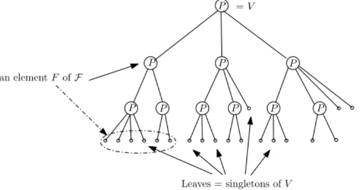
This type of family is called laminar. No two elements of F overlap, and thus it is straightforward to see that such a family can be represented by a rooted tree, such that
• the leaves of this tree are in bijection with elements of V ;
• the nodes of this tree are in bijection with elements of F in the following way: each node of the tree represents the subset of V consisting of all elements corresponding to leaves of the subtree rooted in this node.
Figure 1 illustrates this simple example. Partitive families are a more evolved example.
P P P P P P P P P P an element F of F = V Leaves = singletons of V
Fig. 1. Tree representation of a laminar family.
Definition 2. A family F of subsets of V is partitive if
• V and all singletons belong to F
• for all X, Y ∈ F such that X overlaps Y , X ∪Y , X ∩Y , and (X \Y )∪(Y \X)
are also in F.
Notice that laminar families are a special kind of partitive family, and the tree representation of partitive families that follows generalizes that of laminar.
A partitive tree is a rooted tree T whose internal nodes are labelled Prime or
Complete, and whose leaves are labelled in bijection with the elements of V . We
• For every Prime node of the tree : the subset of V consisting of all elements corresponding to leaves of the tree that are descendants of this node, • for every Complete node, and for every possible union of its children : the
union of the subsets of V represented by these children, • for every leaf of the tree : the corresponding singleton.
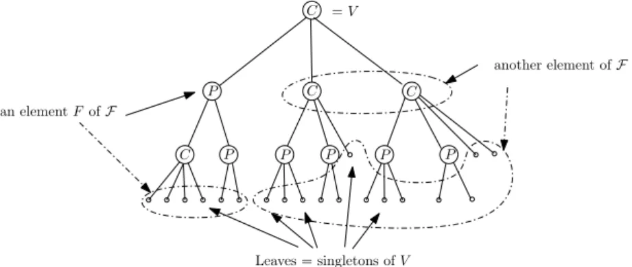
Figure 2 shows a partitive tree. The following theorem states that every partitive family can be represented this way.
Theorem 3. [3, 19, 13] A partitive family can be represented by a partitive tree.
Note that there is an ambiguity about nodes with two children, they may be labelled Prime or Complete, but in this paper we always choose to label them as Complete. C P C C C P P P P P an element F of F = V Leaves = singletons of V another element of F
Fig. 2. Partitive family
We present now another way of seeing partitive families. It is related to the central notion of this section, that is defined below.
Definition 4. Let F ⊂ 2V be a family of subsets of V . Its orthogonal, denoted
by F⊥, is defined by
F⊥ = {X ⊆ V | ∀ Y ∈ F, X⊥Y }.
The following results are easy to prove. Proposition 5. (F ∪ F′)⊥ = F⊥∩ F′⊥
Proposition 6. F⊥ is a partitive family.
Proposition 7. If F is partitive, then the tree representation of F⊥ is obtained
from that of F by switching Prime and Complete nodes.
Corollary 8. If F is partitive, then F⊥⊥ = F. Therefore, every partitive
family F is the orthogonal of some family F′
After these definitions, we can show the main result in this section. Given a general family F, the following theorem of McConnell states that it is possible to compute the tree representation of its orthogonal in an efficient way.
Theorem 9. [15] Given a family of subsets F, it is possible in O(kFk) time to compute the partitive tree representation of F⊥.
It should be noticed that the linear time algorithm in [15] for computing the orthogonal of a general family F is mainly based on an algorithm of Dahlhaus for
computing overlap classes, presented in [8]. This last algorithm has been recently revisited, simplified, extended and implemented in [2, 21]. The main computational insight is that although the overlap graph of F can be of quadratic size, the overlap components can be computed in O(kFk) time.
3. Split Decomposition - Theory. In this section, we show how orthogonals can be used as the main ingredient to compute the split decomposition of undirected graphs. In the rest of the paper, G = (V, E) denotes a simple connected graph. For X ⊂ V , we denote by N (X) its set of neighbours; that is, the set of vertices y 6∈ X such that there exists xy ∈ E with x ∈ X.
3.1. Introduction. We now recall some definitions and previous results on splits, and we define precisely the structure we are aiming for. Some proofs are omitted; for these we refer the reader to the pioneering work of Cunningham (see [6] for more details).
Definition 10. A split of G = (V, E) is a partition of V into two non-empty subsets X1and X2such that the edges between X1 and X2 induce a complete bipartite
graph. In other words, there exists a partition of V into 4 subsets V1, V2, V3, V4, such
that X1 = V1∪ V2 and X2 = V3∪ V4, and such that G contains all possible edges
between V2 and V3, and no other edges between X1 and X2.
We denote splits either by bipartitions (X1, X2) or by quadripartitions (V1, V2, V3, V4)
depending on needs. Both are equivalent since there is a unique quadripartition for each bipartition.
A split is said to be non trivial if both sides have more than two vertices.
2 3
V
1 V V V4
Fig. 3. Structure of a split.
Figure 3 illustrates the notion of a split. A special case of split is the notion of module. Definition 11. A subset M of V is called a module if, using the notations of the previous definition, there exists a split such that V1 = ∅ and M = V2. A module
is strong if it overlaps no other module.
Modules, also called homogeneous sets, appear in various contexts, for example perfect graphs, claw free graphs or in the design of efficient algorithms (see for instance [20, 1]). Their structure is well studied, and a representation of all modules is a tree called a modular decomposition. Given a graph G there are linear O(|V | + |E|)-time algorithms to compute this decomposition [5, 18].
A graph may contain an exponential number of splits. For instance in a complete graph every bipartition is a split (in fact a module). However all splits may be represented in a compact way. This is where the notion of a strong split appears.
Definition 12. Two splits (V1, V2, V3, V4) and (V1′, V2′, V3′, V4′) cross if V1∪ V2
overlaps both V′
1∪ V2′ and V3′∪ V4′. A split is strong if it crosses no other split.
What is fundamental is that the splits have a partitive-like structure.
Theorem 13. [6] Fix r ∈ V (G). {X ⊂ V (G) | (X, V \ X) is a split of G and
r 6∈ X} is a partitive family of V (G) \ {r}
Therefore, adding just an edge with leaf r at the root of the partitive tree rep-resenting this family yields an unrooted tree which represents all the splits of G. Its
leaves are in bijection with V and its set of edges of T are in bijection with the strong splits of T in the following way : with each edge e of T is associated the bipartition of V given by the labels of the leaves of the two connected components of T − e. Moreover, Cunningham’s decomposition theory builds an object that is more precise than just the tree mentioned above by adding labels to its internal nodes.
Definition 14. Suppose V (G) admits a partition (V1, V2, . . . , Vk) such that each
(Vi, V (G)\Vi) defines a split of G. Construct a graph Q with k vertices (v1, v2, . . . , vk)
and with an edge vivj if and only if G contains an edge between Vi and Vj.
The graph Q is called the quotient graph with respect to this partition into splits.
An important result is the following.
Proposition 15. [6] Suppose V (G) admits a partition (V1, V2, . . . , Vk) such that
each (Vi, V (G) \ Vi) defines a split of G. Let Q be the quotient graph associated with
this partition.
If A = {vi| i ∈ I} defines a non trivial (resp. strong) split (A, V (Q) \ A) of Q for
some I ⊂ {1, . . . , k}, then (∪i∈IVi, ∪i6∈IVi) is a non trivial (resp. strong) split of G.
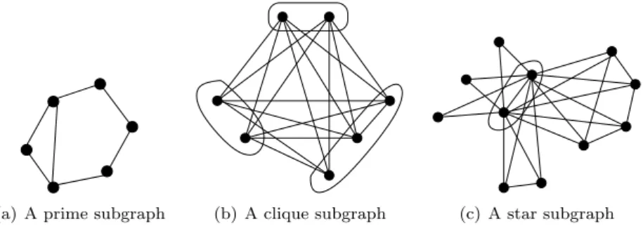
What this implies is that if we dispose of a tree representing all strong splits of the graph, there are only few possible cases for the nodes. Given a node of this tree, by removing it we get a family of subtrees, and thus a partition of the vertex set of G. Using the notations of the previous proposition, either the quotient graph Q associated with this partition is a prime graph (it contains no non trivial splits), and in which case no union of the Vi defines a split of the graph, or it contains some non
trivial splits but no strong one. In the latter case it is not difficult to prove that the graph Q is either a clique Kn, or a star K1,n. In both cases, all possible unions of
the Vi define a split with respect to their complement. Figure 4 shows an example of
these three cases.
(a) A prime subgraph (b) A clique subgraph (c) A star subgraph
Fig. 4. Examples of the three distinct type of nodes of Cunningham’s tree. The center of the star is encircled.
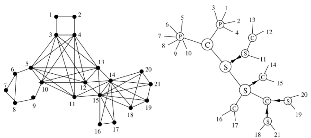
The whole tree, with its nodes labelled Prime, Star or Clique (corresponding to the three possible cases described in the previous paragraph) and the orientation associated with each Star node to point to its centre, forms the Cunningham’s de-composition tree and is the structure we are building in the rest of the paper. An example of such a tree is given in Figure 5. Our approach is first to fix an arbitrary vertex r as a root in our graph and then use Theorem 13 to find all parts of strong splits that do not contain r. The previous discussion implies the following result of Cunningham.
Proposition 16. [6] Let (X, Y ) and (X′, Y′) be two crossing splits, there exists
either a Star (V0, V1, . . . , Vk) or a Clique (V0, V1, . . . , Vk) and ∅( I, I′ ( {1, . . . , k}
C S P P S 1 3 4 5 6 7 8 9 10 11 12 13 14 15 16 17 18 19 20 21 2 16 17 14 15 11 13 12 3 1 2 4 5 6 7 8 10 9 S C C C 21 18 19 20 S S C
Fig. 5. An example of graph and its corresponding split tree. Nodes labelled C, S and P are respectively clique, star and prime. An orientation is associated to each star node to point its center. Note that nodes with 3 incident edges could have been labelled prime
3.2. Split Borders. Let r be a vertex of G. For each split (V1, V2, V3, V4)
(us-ing notations of Definition 10), r lies either in V1∪ V2 or in V3∪ V4. Without loss of
generality, we consider that for all splits we have r ∈ (V1∪ V2). The root vertex r
then allows us to “orient” every split.
Notations: The set V3∪ V4 is called the split bottom and the set V3 is called the
border of the split (V1, V2, V3, V4). Notice that two different splits bottoms may share
the same border.
We define the distance of a split bottom (resp. border) S as its distance from the root, that is minx∈Sd(r, x). We denote G[h] as the subgraph induced by the vertices
at distance h, and G[≤ h] as the subgraph induced by the vertices at a distance of h at most, and similarly G[< h] or G[> h] in the obvious way. For X ⊂ G[> h] we denote Nh(X) as the set N (X) ∩ G[h]. Moreover, the letter H always denotes the set
of vertices of G[h]. Note also that all orthogonal notations here refer to the orthogonal with respect to the ground set H.
Lemma 17. All vertices of a border B are at the same distance from the root r.
This justifies the approach of our algorithm: we first compute (using a breadth first search for example) the distance layers of our graph, and then we process one layer after the other in a bottom-up approach from the furthest layer to the first one. At each step, we need to identify the set of borders at distance h from the root r.
Let us denote by Bh the set of all borders of split at distance h from the root
r. Let C1, . . . , Ck be the connected components of G[> h]. We define two families of
subsets of H:
• M = {modules of G[≤ h] that are subsets of H}, • V = Ski=1Vi
where Vi= {N (Ci) ∩ H} ∪ {N (x) ∩ H | x ∈ Ci} ∪ {(N (Ci) \ N (x)) ∩ H | x ∈ Ci}.
Theorem 18.
Bh= M ∩ V⊥
Proof. We use the notations (V1, V2, V3, V4) of Definition 10 to denote the different
is in fact a module of G[≤ h]. Thus B has to be an element of M.
Now consider a connected component Ci. Either it is included in V4in which case all
elements of Viare clearly subsets of B, or it is included in V1∪ V2. In the latter case,
the vertices in V1 have no neighbour in B and the vertices in V2 see all elements of
B. This implies that B ∈ V⊥.
Conversely, assume B ∈ M ∩ V⊥. Let V
3 = B and let V4 be the union of all Ci
of G[> h] such that (N (Ci) ∩ H) ⊂ B. Let V′= V \ (V3∪ V4). For every x ∈ V′,
• either x belongs to some Ci. Since B ∈ V⊥, B does not overlap N (x) ∩ H
nor its complement in N (Ci). Thus x sees all vertices of B or no vertex of B;
• or x belongs to no Ci. Then x ∈ G[≤ h]. Since B ∈ M, x either sees all
vertices of B or no vertex of B.
We then define V1= V′\ N (B) and V2= V′∩ N (B). Clearly (V1, V2, V3, V4) is a split,
and thus B is a border.
Theorem 19. Bh∪ {H} = (M⊥∪ V)⊥ and Bh∪ {H} is a partitive family
Proof. First, recall that all orthogonals are taken with respect to the ground set
H. M ∪ {H} is a partitive family. Indeed the union, intersection and symmetric difference of two overlapping modules A and B contained in H are modules contained in H. However H may fail to be a module, and thus may fail to be a split. To handle this case we apply Proposition 5:
Bh∪ {H} = (M ∩ V⊥) ∪ {H} (by previous theorem)
= (M ∪ {H}) ∩ (V⊥∪ {H})
= (M ∪ {H})⊥⊥∩ (V⊥) (by Corollary 8) = ((M ∪ {H})⊥∪ V)⊥ (by Proposition 5)
= (M⊥∪ V)⊥
Proposition 6 shows that Bh∪ {H} is partitive.
This theorem is the core of our algorithm to compute Cunningham’s split decom-position tree. Note that since Bh∪ {H} is a partitive family, it can be represented by
a partitive tree, which root corresponds to H. Therefore, Bhcan be represented by a
forest, obtained from this tree by possibly removing the root if H 6∈ Bh.
3.3. Split Bottoms. In the previous section we explained the structure of the split borders of each layer. We consider now split bottoms, which are related both to split borders and to connected components. The following proposition and its corollary below are consequences of the proof of Theorem 18.
Proposition 20. Let B be in Bh. If C is a connected component of G[> h],
there are only 3 possible cases:
1. Nh(C)* B. In this case C is not included in any split bottom with border B.
2. Nh(C) ⊂ B and there exists x in C such that ∅( Nh({x})( B. In that case
C is in every split bottom with border B.
3. C is a split bottom of distance h + 1 and Nh(C) = B. Then to every split
bottom with border B that does not contain C, it is possible to add C to get another split bottom with border B.
According to the case, C is said to be of Type 1, Type 2 or Type 3 with respect to B. We call strong split bottom the bottom of a strong split. We have:
with border B. These are: B ∪ [ C of Type 2 C and B ∪ [ C of Type 2 or 3 C
where C denotes a connected component of G[> h].
We introduce now a definition and a proposition in order to clarify the link be-tween being a strong border (a border that overlaps no other border) and being the border of a strong split.
Definition 22. Let (V0, V1, . . . , Vk), k ≥ 3 be a partition of V (G) such that each
(Vi, V (G) \ Vi) defines a split of G. If the quotient graph is a star with centre V0,
and if r does not belong to V0, this partition into splits is called a bad star (and a
good star if V0contains r). If (w.l.o.g.) r belongs to V1, then ∪i≥2Vi is clearly a split
bottom and its border is called a bad star border.
Proposition 23. If B is in Bh∩ Bh⊥ (a strong border), then B is the border of a
strong split if and only if it is not a bad star border. Furthermore, if B is a bad star border, then no other border strictly contains B and no component of G[≥ h] has an intersection with H that strictly contains B.
Proof. First suppose that B is a bad star border, at distance h from r. The
centre is V0, V1 is the ray that contains r and V2...Vk are the other rays. Consider
a split bottom with border B. Since k ≥ 3, every Vi, i ≥ 2 is included in this split
bottom, while V0 and V1 are on the other side of the split. Therefore, only one split
has border B, namely (V0∪ V1, V2∪ ... ∪ Vk). It is weak since it is crossed by split
(V2∪ V0, V1∪ V3∪ ...Vk).
Conversely let B be a strong border (i.e. in Bh∩ B⊥h) which is not the border of a
strong split. We shall prove that B is a bad star border. As each border is the border of at least one split, then B must be the border of at least two weak splits.
From Proposition 16 we know that these weak splits are in Clique or Star con-figuration into V0...Vk. First, let us study the case where the split is either in Clique
configuration or in Good Star configuration. Without loss of generality we can assume that r ∈ V0 (in the good star case it means that V0 is the centre of the star). For
i > 0, let V′
i be the vertices of Vi incident with V0. Then any union of Vi′ is a border.
Therefore only the maximal union B = V′
1∪ ...Vk′is a strong border. Then B ∩ V0= ∅
but for i > 0 B ∩ Vi 6= ∅. Split (V0, V1∪ ...Vk) has border B and is strong. This is a
contradiction.
So we are left with the Bad Star configuration case (we still assume V0to be the
centre, so r /∈ V0). Let B be a bad star border contained in a larger bad star border
B′. B′ is not connected in G[≥ h] and each connected component corresponds to a
ray of the star. Some of them belong to B, others do not. A combination of such rays overlaps B, which can not be a strong border. So B is maximal with respect to inclusion. The last claim of the proposition comes from the fact that a bad star border has no neighbour inside G[h] (these neighbours would have to be in the centre of the star and therefore would be connected to some elements of the upper ray V1,
which is not possible since these elements belong to G[h − 2]).
4. Split Decomposition - Algorithm. In this section, we show how the theory developed above combined with the algorithm for computing the orthogonal of a family (Theorem 9) allows us to design a O(|E|)-algorithm to produce Cunningham’s tree decomposition. The exact complexity analysis is postponed to §5.
4.1. Building the tree decomposition - General Approach. Our algorithm constructs Cunningham’s tree of strong splits in a step by step “bottom up” approach. At each step of our algorithm we produce a forest Fh of rooted trees which roughly
represents all labelled split bottoms at distance at least h, for h going down to 1. From now on, we call internal nodes of this forest the nodes which are neither leaves, nor roots. As in Cunningham’s tree, the leaves of our forest are labelled with the vertices of the graph (each vertex is associated with at most one leaf), and each non-leaf node is associated with a subset of V (G), which are the labels of the descendants of this node. We say that this node represents this set. Sometimes, to simplify notations and if no confusion may occur, we will identify a node with the set it represents.
The following invariants are maintained after processing layer h:
Invariant 1 The leaves of Fh are exactly labelled by the vertices at distance
greater or equal to h (vertices of G[≥ h]).
Invariant 2 Each strong split bottom at distance greater or equal to h is rep-resented by one node of Fh.
Invariant 3 Each internal node of Fh represents a strong split bottom and is
given with its correct label Star, Prime or Clique.
Invariant 4 Each root of Fhrepresents either a connected component of G[≥ h]
that is not a split bottom, or a connected split bottom (in that case it is labelled either Clique or Prime) or a split bottom that is the union of several such connected components (and in that case it is labelled Star).
The algorithm constructs the forest Fh from Fh+1by adding new leaves (vertices
of G[h]) and new nodes. For h = n the initial forest is empty and this algorithm continues until h = 1. Notice that (V (G) \ r) is a strong split bottom and therefore has to be represented by a node P in F1 (Invariant 2). This implies that the forest
F1 is in fact a unique tree and the node P is the root of this tree. By adding r as a
leaf attached to P , P and all internal nodes represent a strong split bottom (Invariant 3), and all split bottoms are represented by a node (Invariant 2). Therefore, this last tree is that of Cunningham.
Thus, we only need to show how to construct Fh from Fh+1while preserving these
four invariants.
The following point is important. Assume that we want to process layer h and compute Fh from Fh+1. Since we maintain Invariant 2, i.e. each split bottom at
distance h is represented by a node of the forest, and since split bottoms at distance h+1 or more are already represented, we only need to be concerned about split bottoms
at distance exactly h, i.e. split bottoms with borders included in the layer G[h]. Thus,
the leaves we add are exactly the vertices of G[h], and, as explained below, the internal nodes we add correspond exactly to the bottoms.
4.2. Recursive Computation of Fh. In this section we explain how to build
the forest Fh from the two forests Fh+1 and the forest representing all borders in
Bh. To simplify notations in the rest of the paper, we will identify Bh with the forest
representing it.
After computing Bh (see §5), we need to slightly transform it to consider the
connectivity inside layer h (maintaining Invariant 4). Let us call h-component the intersection of a connected component of G[≥ h] with H. We build the forest B′
following way: each tree of Bh is incorporated in B′h. Then, for each h-component
that contains the roots of at least two trees, we create a new node corresponding to this h-component, with these roots as children. We do not need to give a label to this new node as it will be merged with another node during the algorithm. Furthermore we change the type of all complete node of Bhto either Clique or Star. Let N be such
a complete node and S1, S2 two of its children, and pick two vertices x1 ∈ S1 and
x2∈ S2. If they are adjacent, then N is relabelled Clique, otherwise it is relabelled
Star. If N is Star and has a parent then the centre of the star is that parent (otherwise,
it will be defined later). For correctness of the labeling see the proof of Invariant 3. We need the following result to properly state the algorithm.
Proposition 24. Let C be a connected component of G[> h]. Then Nh(C) is
contained in at least one node of B′
h (i.e. is in the vertex-set of G[h] represented by
this node).
Proof. All elements of Nh(C) belong to the same h-component.
Notations: Notice that a forest is defined by a parent relation between nodes, unde-fined for roots. We perform three kinds of operations which modify a given forest.
• Merging Node A with Node B means setting each child of A as a new child of B and removing A (notice that it is not commutative).
• Linking A to B sets parent(A) := B.
• Adding a parent to node A consists of creating a new node B, then setting parent(B) := parent(A) and then parent(A) := B.
Remark: Thanks to Invariant 4, we know that a root of Fh+1 represents either one
connected component of G[> h] or a union of connected components that have the exact same neighbourhood in G[h]. Therefore, all the results of §4.2 and §4.3 are perfectly valid if we replace the family of connected components of G[> h] by the family of roots of Fh+1. Then we use the terminology of Proposition 20 for a root
R of Fh+1 (instead of a component C) and call it Type 1, Type 2, or Type 3 with
respect to some given border in Bh.
Algorithm computing Fh from Fh+1.
1. Compute Bh(using Theorem 18, see §5.3).
2. Compute B′
h(as described above)
3. For each root R of Fh+1, let B be the lowest node of Bh′ such that Nh(R) ⊂ B.
(a) If R is a not a split bottom (R is just a connected component of G[≥ h]), then merge R with B. The label of B does not change.
(b) Else if R is of Type 2 with respect to B, or if B is not a split border, then link R to B. If R is labelled Star, then orient the edge from R to B.
(c) Else if R is of Type 3 with respect to B and R is labelled Star then add a parent P to B and merge R with P . Label P Star and orient the edge P B from P to B.
(d) Else (R is of Type 3 with respect to B but not labelled Star) add a parentP to B and link R with P . Label P Star and orient the edge P B from P to B.
4.3. Correctness. As noted previously, we just need to prove that Invariants 2,3 and 4 are still true after the update.
Invariant 2. The only nodes of Fh+1 that are destroyed during the update are the
roots that we merge. We do this only in two cases. Either when the root is a connected component but not a split bottom – and in that case it is not a problem (and it is
needed by Invariant 3) – or when the root is labelled Star, which by Invariant 4 implies that it represents a disconnected split bottom, and its neighbourhood in G[h] is a split border. This is exactly the case of a bad star, and thanks to Proposition 23, we know this node had to be deleted (they do not represent strong bottoms). So we preserved all strong split bottom of distance at least h + 1.
Now we need to prove that this invariant is also true for strong split bottoms at distance h. Such a strong split bottom S has its border BS in Bh∩ B⊥h, which means
that it is represented by a node N in Bh. Thanks to Corollary 21, we know that at
most two strong split bottoms with border BS can exist, BS along with components
of Type 2, and BS along with components of Type 2 and 3. With respect to BS every
root of Fh+1 is either of Type 1, 2, or 3. Type 1 components are never placed by the
algorithm under node N , since their neighbourhood is not included in BS. Type 2
components are always put under N , since N is either B or an ascendant of B, where B is the smallest node containing their neighbourhood. Therefore, in Fh the vertices
below node N are exactly BS, along with Type 2 components. Finally, if any Type
3 components exist for BS, then the algorithm creates a new node P in Fh. The
vertices below this node P in the end are exactly BS with all components of Type 2
and of Type 3.
Invariant 3. Let N be an internal node of Fh. There are three possible cases
resulting from the update algorithm:
1. N comes from a node of Fh+1 (either internal or a root that has not been
merged).
2. N is created by add a parent. 3. N comes from a node of B′
h.
If N comes from an internal node of Fh+1, since the subtree rooted in N has not
been modified by the update, by Invariant 3 in the previous step we know that it represents a strong split bottom at distance greater than h. If N comes from a root of Fh+1 and has not been merged (cases (b) and (d) of the algorithm), this means that
it represents a maximal split bottom of distance greater than h that is not a bad star bottom, since case (a) deals with R not split bottom and case (c) deals with R bad star border with ≥ 3 rays. Therefore by Proposition 23 N represents a stong split bottom.
If N is a node that was created by an add a parent operation, this means that it represents a split border along with all components of Type 2 and 3 with respect to it. This is also the case with a strong split bottom.
Eventually, if N comes from a node of B′
h and is internal, then N represents a
border along with its Type 2 Components. Indeed, the only nodes in B′
h that do
not represent borders are the roots added to Bh during the creation of Bh′ but the
algorithm never adds a parent to those, so they remain roots. Therefore we know that N represents a split bottom, and we need to prove that it represents a strong one. Thanks to Proposition 23, we know that if a split bottom is not strong but has a border in Bh∩ B⊥h, then this border must be a root of B′h. Notice also that the
update algorithm never adds a parent to such a root since it only does so if there exists a component of G[> h] of type 3 with respect to it (and therefore connecting all of them), but this is not possible in the case of a bad star border since every ray is in a different connected component of G[≥ h]. Therefore, these split bottoms can only be represented by roots of Fh.
that the node labelling is correct. From Proposition 16 we know the labels have to be Prime, Clique or Star. If an internal node comes from Bh, then it had a Prime or
Complete label. A split bottom is Prime if and only if no proper union of its children defines a split bottom, and therefore, if and only if its border is a prime border. Moreover, recall that for a given split bottom, if some union of its children defines a split bottom (it is labelled Complete in Bh), then any union does and in that case
it is Clique if and only if it is connected, and Star if every child defines a connected component. These conditions are exactly the ones we apply when transforming the labels of Bh into the ones of B′h.
If the internal node comes from Fh+1, since labels are unmodified, the validity is
guaranteed by the Invariants in the previous step.
Eventually, if the internal node comes from an add a parent operation, it means that it represents a star split bottom (it has a component of Type 3) whose centre is the part containing the border and is thus labelled accordingly.
Invariant 4. By construction, roots of Fhare of three kind:
1. either they come from a root of Bh,
2. or they were added during the construction of B′
h(because of a h-component),
3. or they were added to some root of the first kind during the update because of Type 3 components (we do not apply add a parent to nodes that represent h components).
In the first or third cases, such a root represents a split bottom and is well-labelled for exactly the same reasons as for internal nodes (see proof of Invariant 3). In the second case, it is not a split bottom and thus receives no label. Note that from the definition of B′
h, if we denote by A a root of B′h and C is a connected component of
G[> h], either C is of Type 2 or 3 with respect to A, or Nh(C) ∩ A = ∅. This clearly
implies that when A becomes a root of Fh it represents a connected component of
G[≥ h].
5. Split Decomposition - Implementation and Complexity. Let Eh
de-note the set of edges in G[h] and Eh,h+1 the set of edges between G[h] and G[h + 1].
The efficiency of the whole algorithm relies on the fact that the update algorithm on layer h runs in time proportional to |H| + |Eh−1,h| + |Eh| + |Eh,h+1|, which is proved
below.
Recall that there are three steps in the update algorithm. The first step concerns the computation of Bh and is the main subject of this section. It relies on Theorem
18 and therefore on the computation of orthogonals, modular decomposition and connected components. In general, the former can be handled using the algorithm of McConnell (see §2).
However, the problem here is that the sizes of the families of §4 might not be linear in the size of the underlying graph. We will show below how to deal with this difficulty by computing smaller families with the same orthogonals. The modular decomposition aspects are explained in §5.3. Computing the connected components of G[≥ h] for all h is also clearly linear in the number of edges of the graph. Since these connected components are the only information needed to compute B′
hfrom Bh
this implies that the second step of the update algorithm is also linear.
The third step, computing Fhfrom Fh+1and B′h, can be done in linear time using
classical algorithmic operations on trees. Indeed for every root R of Fh+1(recall that
we identify R with the set of vertices it represents), we need to identify the lowest node B of B′
in B′
h of the neighbours of R in G[h] and can be done by a bottom-up exploration in
this tree. For every such R this takes time proportional to the number of edges of G between R and G[h].
5.1. Computing M.
Theorem 25. [26, 17, 5] Modules of a graph G = (V, E) form a partitive family whose associated tree can be computed in time O(|V | + |E|)
Let G[h − 1, h] denote the graph induced by the vertices at distance h − 1 or h from the root.
Corollary 26. Computing the partitive tree representing M ∪ {H} can be done in time O(|V (G[h − 1, h])| + |E(G[h − 1, h])|.
Proof. The family M is exactly the family of modules of G[h − 1, h] included in
G[h]. So, in time proportional to the size of G[h − 1, h], its modular decomposition (the partitive tree) can be computed. Then the leaves labelled by vertices in G[h] are marked. We then perform a bottom-up selection : for each node whose children have been processed, we distinguish four cases.
• If all its children are marked, then the node is marked. • Else if no children are marked, then the node is deleted.
• Else if the node is labelled Complete then we delete all unmarked children. Furthermore, if only one child remains, then we merge the node with its child. • Else (it is labelled Prime), the node is deleted.
Note that this process yields a forest if H is not a module. In that case, we add a root to get the desired partitive tree.
An important property for the time complexity of our algorithm is: Proposition 27. kMk = O(|Eh−1,h| + |Eh| + |H|).
Proof. This fact directly derives from that the total sum of all elements of all
strong modules of a graph G is O(n + m) as proved in [16].
5.2. Efficient Computation of Overlaps in Two Particular Cases. We de-scribe here two tools that allow us to efficiently compute orthogonals in two particular cases. Both are of use for assessing the linear complexity of the algorithm.
Lemma 28. Let V = {x1, x2, . . . , xp} be a finite set. Let A = {{xi, xi+1} , i =
1 . . . p, and xp+1= x1}. Then A⊥= (2V)⊥ = {{xi}, i = 1 . . . p}
As a consequence, let us consider a prime node of a partitive tree with children A1, . . . Ap. We know that it is the orthogonal of its associated Complete node, i.e.
the family of all possible unions of sets Ai. What the lemma says is that it is also
the orthogonal of the family with p elements of this type: Ai∪ Ai+1, and this family
is much smaller than all possible unions, since its norm is twice the norm of the Ai.
We call {A1∪ A2, A2∪ A3. . . Ap∪ A1} the circulant family associated with the Ai.
Schematically, this can be graphically represented as the ”equality” Figure 6.
A1 A2 A3 A4 A5 A6 A7 A8 A1 A2 A3 A4 A5 A6 A7 Complete Node A8 A1 A2 A3 A4 A5 A6 A7 Prime Node A8
Fig. 6. A circulant family and its orthogonal.
Proposition 29. Let F be a family of subsets of V . Given the partitive tree
and such that the size of H and the time needed to do this calculation are proportional to the size of this tree, that is
F⊥⊥∩ F⊥ .
Proof. The family H is simply the family containing the sets represented by the
nodes of the tree (i.e. elements of F ∩ F⊥) plus, for each prime node of this tree, the
circulant family associated with the children of this node.
We use this result to prove another proposition used in the next section.
Proposition 30. Let V be a finite set, and X be a subset of V . Assume that
F is a family of subsets of X such that X ∈ F. Let us define a new family H by H = F ∪ {X \ F | F ∈ F}. Then in time O(kFk), it is possible to compute a family H′ such that H′⊥= H⊥ and whose size is O(kFk).
Proof. Let P1, · · · , Pt be the equivalence classes of the following relation on
ele-ments of X: x and y are equivalent if they belong to the same members of the family H. The sets Pi thus form a partition of X and we define H′, as in Figure 6, as:
H′= {P
i∪ Pi+1, i = 1, . . . , t − 1} ∪ {Pt∪ P1}
Both H′⊥and H⊥ are equal to the family of subsets A of V such that either
1. there exists (a unique) i such that A is included in Pi, or
2. X ⊂ A, or 3. X ∩ A = ∅.
Therefore H′⊥ = H⊥ and it is clear that kH′k = O(|X|). The time complexity
of the construction of H′ depends on the efficiency of building P
1, · · · , Pt. We use
partition refinement that can be carried out by the very simple following process: let U be a family on X, containing only X at the beginning. We consider successively each set Y 6= X in F as pivot. For each C ∈ U such that C = C′∪ C′′, with C′ 6⊂ Y ,
C′′ ⊆ Y, C′ 6= ∅, and C′′ 6= ∅. We only replace C by the two sets C′ and C” in U .
At the end of this process, U is the partition of Pi of X we aim for. This refinement
procedure can be implemented in O(kFk) using a structure based on an augmented array [2] or based on an ad-hoc doubly linked list [12].
5.3. Computing The Family of Borders Efficiently. In this section, we show how to use the tools of §2 and §3 to compute the family of borders Bh
effi-ciently, that is with a linear (with respect to the number of edges of the graph) time complexity. Theorem 19 asserts that
Bh∪ {H} = (M⊥∪ V)⊥.
Of course, we want to apply the orthogonal algorithm of McConnell ([15], see §2). But if we do this directly on the family (M⊥∪ V) the time complexity can be greater
than what we want, because this family can be too large (for instance because of the complements of neighborhoods in family V). To avoid this issue, we use the reduction tools of §5.2. Using the notations of §3.2,
Bh∪ {H} = (M⊥∪ V)⊥= (M⊥)⊥∩ V1⊥∩ V2⊥∩ . . . ∩ Vk⊥
The forest representing the family M can be calculated in time O(|Eh| + |Eh−1,h|).
Then the tree representing M⊥ can be obtained by simply swapping Prime and
Complete nodes as stated in Proposition 7. Now, as the total size of the family
is linear (Proposition 27), using Proposition 29 it is possible to construct in time O(|H| + |Eh| + |Eh−1,h|) a family N such that
Furthermore, using Proposition 30, it is possible, in time proportional to the sum of the sizes of the sets in {N (Ci) ∩ H} ∪ {N (x) ∩ H, x ∈ Ci}, to compute a family Wi
such that:
W⊥ i = Vi⊥.
Let us define W as the union of all Wi. It is important to note that kN k is
O(|H| + |Eh| + |Eh−1,h|) while kWk is O(|H| + |Eh| + |Eh,h+1|). Now,
Bh∪ {H} = (M⊥)⊥∩ V1⊥∩ V2⊥∩ . . . ∩ Vk⊥
= N⊥∩ W⊥
1 ∩ W2⊥∩ . . . ∩ Wk⊥
= (N ∪ W)⊥.
Thus, we are able to compute a tree representation of Bh∪ {H} by computing
N ∪ W in a total time O(|H| + |Eh| + |Eh−1,h| + |Eh,h+1|) and by using Theorem 9
in the same time. We have just proved the following theorem:
Theorem 31. The partitive tree representing split borders at distance h can be calculated in O(|V (G[h])| + |Eh| + |Eh−1,h| + |Eh,h+1|) time.
Doing this for all h, we get an algorithm that is linear with respect to the total number of edges in the graph.
Acknowledgment. We wish to thank Vincent Limouzy for his participation in the earlier studies we carried out on this subject.
REFERENCES
[1] A. Brandst¨adt, V.B. Le, and J.S. Spinrad, Graph Classes, SIAM Monographs, 1999. [2] P. Charbit, M. Habib, V. Limouzy, F. de Montgolfier, M. Raffinot, and M. Rao, A note
on computing set overlap classes, Information Processing Letters, 108 (2008), pp. 186–191. [3] M. Chein, M. Habib, and M. C. Maurer, Partitive hypergraphs, Discrete Mathematics, 37
(1981), pp. 35–50.
[4] S. Cicerone and G. Di Stefano, One the extension of bipartite to parity graphs, Discrete Applied Mathematics, 95 (1999), pp. 181–195.
[5] A. Cournier and M. Habib, A new linear algorithm for modular decomposition, in Trees in algebra and programming (CAAP), vol. 787 of Lecture Notes in Computer Science, Springer-Verlag, 1994, pp. 68–84.
[6] W. H. Cunningham, Decomposition of directed graphs, SIAM Journal on Algebraic Discrete Methods, 3 (1982), pp. 214–228.
[7] E. Dahlhaus, Efficient parallel and linear time sequential split decomposition (extended ab-stract), in Proceedings of the 14th Conference on Foundations of Software Technology and Theoretical Computer Science, London, UK, 1994, Springer-Verlag, pp. 171–180. [8] E. Dahlhaus, Parallel algorithms for hierarchical clustering, and applications to split
decom-position and parity graph recognition, Journal of Algorithms, 36 (2000), pp. 205–240. [9] C. P. Gabor, K. J. Supowit, and W.-L. Hsu, Recognizing circle graphs in polynomial time,
J. ACM, 36 (1989), pp. 435–473.
[10] C. Gavoille and C. Paul, Distance labeling scheme and split decomposition, Discrete Math-ematics, 273 (2003), pp. 115–130.
[11] E. Gioan and C. Paul, Dynamic distance hereditary graphs using split decomposition, in Algorithms and Computation, 18th International Symposium (ISAAC), 2007, pp. 41–51. [12] M. Habib, C. Paul, and L. Viennot, Partition refinement techniques: an interesting
al-gorithmic toolkit, International Journal of Foundations of Computer Science, 10 (1999), pp. 147–170.
[13] W.-L. Hsu and R. McConnell, PC-trees and circular-ones arrangements, Theoretical Com-puter Science, 296 (2003), pp. 99–116.
[14] T. Ma and J. P. Spinrad, An O(n2) algorithm for undirected split decomposition, Journal of
Algorithms, 16 (1994), pp. 145–160.
[15] R. McConnell, A certifying algorithm for the consecutive-ones property, in SODA, 2004, pp. 768–777.
[16] R. McConnell and F. de Montgolfier, Linear-time modular decomposition of directed graphs, Discrete Applied Mathematics, 145 (2005), pp. 198–209.
[17] R. McConnell and J. Spinrad, Linear time modular decomposition and efficient transitive orientation of comparability graphs, in Proceedings of the fitth Annual Symposium on Discrete Algorithms (SODA), 1994, pp. 536–545.
[18] R. M. McConnell and J. P. Spinrad, Linear-time modular decomposition and efficient tran-sitive orientation of comparability graphs, in SODA ’94: Proceedings of the fifth annual ACM-SIAM symposium on Discrete algorithms, SIAM, 1994, pp. 536–545.
[19] R. H. M¨ohring, Algorithmic aspects of the substitution decomposition in optimization over relations, set systems and boolean functions, Annals of Operations Research, 6 (1985), pp. 195–225.
[20] R. H. M¨ohring and F. J. Radermacher, Substitution decomposition for discrete structures and connections with combinatorial optimization, Annals of Discrete Mathematics, 19 (1984), pp. 257–356.
[21] M. Rao, Set overlap classes computation, source code, 2007. freely available at http: // www.
liafa. jussieu. fr/ ~ raffinot/ overlap. html .
[22] , Coloring a graph using split decomposition, in Graph-Theoretic Concepts in Computer Science (WG), vol. 3353 of Lecture Notes in Computer Science, 2004, pp. 129–141. [23] , Solving some np-complete problems using split decomposition, Discrete Applied
Math-ematics, 156 (2008), pp. 2768–2780.
[24] J. Spinrad, Recognition of circle graphs, Journal of Algorithms, 16 (1994), pp. 264–282. [25] R. E. Tarjan, Decomposition by clique separators, Discrete Mathematics, 55 (1985), pp. 221–
232.
[26] M. Tedder, D. G. Corneil, M. Habib, and C. Paul, Simpler linear-time modular decompo-sition via recursive factorizing permutations, in Automata, Languages and Programming, 35th International Colloquium (ICALP), 2008, pp. 634–645.