PART IV OF IV
ANALYSIS OF PUMPING SYSTEMS FOR
THE COOLING OF UNDERGROUND TRANSMISSION LINES
by Paul F. Koci Leon R. Glicksman Warren M. Rohsenow Energy Laboratory in association with Heat Transfer Laboratory, Department of Mechanical Engineering
MASSACHUSETTS INSTITUTE OF TECHNOLOGY
Sponsored by
Consolidated Edison Co. of New York, Inc. New York, New York
Energy Laboratory Report No. MIT-EL 74-006 Heat Transfer Laboratory Report No. 80619-90
ABSTRACT
Various pumping arrangements and their pressure profile control for forced cooling of long pipe type transmission lines were investigated.
In order to overcome the extensive friction head losses and provide ample cable cooling, a number of pump stations has to be used. Since the inner line segments cannot be provided with pressure
control head tanks, line blockages, flow resistance changes, flow rate changes, pump shutdowns, or other imbalances in: one segment can alter the pressure profile along the entire line, and, when two head
tanks are used, create transverse flow.
Using experimental and analytical methods, it was determined that the pump - relief valve combination operating as a constant flow source is superior to the pump - relief valve combination oper-ating as a constant pressure source, and that the configuration consisting of an even number of loops, each loop having the opposite flow direction from its neighbor's, is the best solution when oper-ated with only one pressure control head tank.
The simplest, and yet effective, line pressure profile cont-rol appears to be the pump bypass, which could be easily implemented on existing installations. The head tank pressure adjustment, how-ever, is the most effective line pressure profile control scheme, and should be considered when a new system is being designed. From the analysis performed on an electric analogy model it was found, that the head tank pressure adjustment or the pump bypass would be suf-ficient to mainain the line pressure profile within its working limits for all practical imbalance sizes, and that, to extend the range of either of these line pressure profile controls, the emergency pump shutdown and the pump bypass itself should be based on the pump discharge, rather than the pump inlet pressure.
This work has been sponsored by the Consolidated Edison Co. of New York, N.Y., Inc.; this support is greatly appreciated.
We are indebted to Mr. Michael D. Buckweitz of Consolidated Edison Co. for sharing his experience and numerous ideas.
We would also like to thank Dr. Howard Feibus of Consolidated Edison Co. for his help.
TABLE OF COW9NTS
Abstract
2
Acknoledgements
3Table of oontents
4
List of figures
7
List of Tables
14
Nomelature
15
1. Introduction 192. Description of the operation and the characteristics of the
present Dunvoodie - Rainey system
24
3.
Survey of possible solutions
27
3.1. System oonfigurations
29
3.1.1.
Configuration
1
29
3.1.2. Configuration 2 29 3,1.3. Configuration 3 33 3.1.4, Configuration 4 33 3.1.5. Conclusion ' 363.2. Line pressure profile control 36
3.2.1. Pump pressure relief valve as the pup discharge
and inlet pressure control 37
3.2.2. Head tank pressure adjustment as the total line
pressure profile control 39
3.2.3. Pump shutdown a emergency pup discharge
3.2.4. Pp
bpass as the pump discharge and inlet
presure ontrol
44
3.2,5. Artificial line blookae as the p discoharge
and inlet pressure control
45
3.2.6. Conclusion
47
4. Steady state
imlation
by the electric
analogy method
48
4.1 Comparison of prototype and model functional relationhips
48
4.11. Characteristics of positive displacement
pups
50
4.1.2. Pipe flow at steady state
55
4.1.3.
ead tank modeling
57
4.1.4. Elevation modeling
58
4.2. le1tronic omoeat
and ircuits ued n modeling
58
4.2.1. Pipeline netwk modeling
61
4.2.2.
Pump modeling
61
4.2.3.
ead tank modeling
65
4.2.4. Voltage
ta
65
4.2.5. Current au
m ts
67
5. Eperiental
program and reults
69
5.1, Imbalane effects on Configuration I with constant
pressure
ources
71
5.1.1. Line blockages
72
5.1.2. Pp
hutdown
73
5.2. Ibal
effects on Configuration 1 ith constt
flow sources
75
5.3.
Cparison of effectiveness of
imbaslance
control in
constant pressre
ource and constant flow source
ssten
75
6. Genetralisation of the
Ine
efects
on Config.
& 2
116
7. Transient effeots during a p start-p
119
8. Conclusions and reomeadations
-
optimal design
125
Appemdix A -
Ror
analysis
129
Appendix -
Effect of line blockages
on
Comfig. 1
136
LIST OF FIGURES
Pig,
1. Configuration
with
mp
- relief valve
ngement
as onstant presr
soures
30
Fig. 2. Configuration with pup - relief valve age
nt
as
oonstant
flow sources.
31
Fig. 3. Configuration 2 with pup relief valve rra
et
as constant flow saurces
32
Fig.
4. Configuration 3 with constant flow soures
34
ig.
5. Configuration 4 with constant flow soures
35
Fig. 6, Comparison of the pup cavitation performance with
the simulated performance
54
Fig.
7. Head tank system used on the' Dunwoodie
-ainey
installation
54
Fig. 8. Caparison of the exaot and ppoxiated
pressre
increase due to elevation
59
Fig.
9. Voltage comparator irmt
60
Fig. 10. Voltage follower circuit
60
Fig. 11. Pump modeling 63
Fig. 12. Coplete pup model
63
Fig. 13. Head tank model
66
Fig. 14. Elevation modeling
66
Fig, 16. Effeot of M2 flow resistance increase of 200% on the
inlet and discharge pressures and the L flowr rate in
Conf.
with FSS (comparison of single pressure ontrol
-
SPC, and dual pressure
ontrol -
DPC)
70
Fig. 17. Simplified model of a loop with constant voltage source
during normal operating oonditions
72
Fig. 18. Effect of the
E1
flow resistane
increase of 100% on
the inlet and discharge pressures and the ML flow rate
in Conf. 1 with single pressure control at the line
left ind (T attaohed to loop #1)
85
Fig. 19. Effect of the
flow esistn
irease
of 200 on
the inlet and discharge pressures and the ML
flow rate
in
Config.
with single pressure control at the line
left end (T attached to loop #1)
86
Fig. 20. Corretion of the HE1 blookage (200% of noxal
E1
flow resistance)
of Fig. 19 by bpassing pump #1
87
Fig. 21, Correction of the El blookage (200% of normal E
flow esistance) of Fig. 19 by increasing the T
pressure (BT attached to loop #1)
88
Fig. 22. Effect of the E1 flow resistance increase of 500% on
the inlet and ischarge pressures and the ML flow rate
in Config. with single pressure control at the line
Fig. 23. Correction of the HE1 blockage (500% of normal HE1
flow resistance)
of Fig. 22 by bypassing pump
#1
90
Fig. 24. Correction of the HE1 blockage (500% of normal HE1
flow resistance) of Fig. 22 by increasing the
HT
pres-sure (T attached to loop #1)
91
Fig. 25. Effect of the HE2 flow resistance increase of 100% on
the inlet and discharge pressures and the ML flor rate
in Config. 1 with single pressure
control
at the
line
left end (T attached to loop #1)
92
Fig. 26. Effect of the HE2 flow resistance increase of 200% on
the inlet and discharge pressures and the ML flow rate
in Config. 1 with single pressure control at the line
left end (T attached to loop #1)
93
Fig. 27. Effect of the
H2
flow resistance increase of 500% on
the inlet and discharge pressures and the ML flow rate
in Configuration 1 with single pressure control at the
line left end (HT attached to loop #1)
94
Fig. 28. Effect of the HE3 flow resistance increase of 100% on
the inlet and discharge pressures and the ML flow rate
in Config. 1 with single pressure control at the line
left end (RT attached to loop #1)
95
Fig. 29. Effect of the HE3 flow resistance increase of 200% on
the inlet and disoharge pressures and the ML flow rate
in Config. 1 with single pressure oontrol at the line
Fig. 30. Effect of the HE3 flow resistance increase of 500% on
the inlet and disceharge pessures and the ML flov rates
in Config. with single pressure ontrol at the line
left end (T attached to loop #1)
97
Fig. 31. Correction of the
1E3
blockage (500% of nomal HE3 flow
resistance)
by bypsing pup #3
98
ig.
32. Correction of the H3 blockage (500% of noml H133
flow
resistane)
of Fig. 30 by increasing the IT presse
(RT attached
to loop #1)
99
ig. 33. Correction of the 3 blockage (500% of nohal flow
resistance of
133)
of ig. 30 by partially bypassing
pup #2)
100
Fig. 34. Effect of the DL1 flow
resistane i
ase
of 30% on
the inlet and discharge pressure and the ML flov rate
in Config. 1 with single pressure control at the line
left ead (
attached to loop 1)
101
Fig. 35. Effecot of the DL1 flow resistance increase of 60% on
the inlet and discharge pressures and he ML flow rates
in Configuration I with ingle pressure oontrol at the
line left end (T attached to loop #1)
102
Pig. 36. Effect of the DL1 flow resintae
increase of 150% on
the inlet and discharge pressures and the L flow rate
in Config. 1 with ingle pressure control at the line
Fig. 37. Effect of the DL2 flow resistance increae of 30% on
the inlet and disch
pressures and the ML flow rate
in Config. I with ingloe pressure control at the line
left
nd (
attached to loop #1)
Fig. 38. Effect of the DL2 flow resistanme
the inlet and discharoge pressures
in Config. 1 with single pressue
left end (
attahed to loop #1)
Fig. 39. Effect of the DL2 flow resistance
the nlet and discharge pressure
in Config.
with single pressuem
left end (
attached to loop #1)
104
increase of 60% oa
and the ML flow rate
control at the line
105
inorease of 150% oa
and the ML flow rate
control at the line
ig,. 40. Correction
of the DL2 blookage (150% an nommal DL2 flow
resistance)
of Fig. 39 by partiallZy bypassing pp
#2
ig. 41. Effect of the MLI flow resistance increase of 40% on
the inlet and disoharge pessures and the ML flow rate
in Config. I with ingle pressure control at the line
left end (T attaohed to loop #1)
Fig.
42. Effect of the NLI flow resistance increase of 80% on
the inlet and discharzge pressures and the ML flow rate
in Config. I with single pressure control at the line
left end (RT attaohed to loop #1)
106
107
108
Fig. 43. Effect of the LI flow resistance increase of 200% on
the inlet and discharge pressures and the L flow rate
in Config. 1 with single pressure control at the line
left end (T attached to loop #1)Fig. 44. Correction of the ML1 blockage (200% of normal ML1
flow
resistance) of Fig. 43 by reducing the T pressure (T
attached to loop #1)
Fig. 45. Effect of the ML2 flow resistance
the inlet and discharge pressures
in
Config.
with single pressure
left end
(T
attached to loop #1)
Fig. 46. Effect of the ML2
flow resistance
the inlet and discharge pressures
in
Config.
with single pressure
left end (T attached to loop #1)
Fig. 47. Effect of the ML2
flow resistance
the inlet and discharge pressures
in Config. 1 with single pressure
left end (HT attached to loop #1)
increase of 40% on
and the ML flow rate
control at the line
112
increase of 80% on
and the M flow rate
control at the line
113
increase of 200% on
and the ML flow rate
control at the line
114
Fig. 48. Correction of the
ML2
blookage (200% of ML2 normal flow
resistance) of Fig. 47 by switching the pressure control
from
the
left
T
to the right one (T attached to loop
#6)110
111
Fig. 49. Plow rate eror due to the linearization as a function
of the loop flow reduction
Figs. 50 - 52. Effect of the HE (4 - 6) flow resistance irease
of 500% on the inlet and discharge pressure ad the ML
flow rate in Config.
with single pressure oontrol at
the line left end (T attached to loop #1)
134
ig. 53 - 56. Effect of the DL (3 - 6) flow resistance increase
of 150% on the inlet and discharge pressums and te
IL
flow rate in Config.
1
with single pressure control at
the line left end (T attached to loop #1)
144
Pigs. 57 - 60. Effect of the
ML
(3 - 6) flow resistance increase
of 200% on the inlet and discharge pressures and the ML
flow rate in Config. with single pressure control at
the line left end (T attached to loop #1)
14
132
7 - 139
0- 143
LIST OF TABLES
Tab. 1.
rSystem
specifications
used in modeling and analysis
25
Tab. 2. Calculated pressure drops using specifications
of Tab. 1
56
NOMENCLATURE
A = cross sectional area
A = nonlinear flow resistance under normal operating conditions A' = linear flow resistance under normal operating conditions a = nonlinear flow resistance
at = linear flow resistance BPS = partial pump bypass D = pump displacement
DL = discharge line or its flow resistance DPC = dual pressure control
DIN = pump shutdown
d = pipe diameter (equivalent pipe diameter) FSS = flow source system
f = friction factor H = pump head
H ma = maximum pump pressure head max
HE = heat exchanger or its flow resistance HT = head tank
LED = light emmitting diode L = pipe length
ML = main cable line (its flow resistance) m = pressure - voltage conversion factor
NOC = normal operating conditions NPSH = net positive suction head
n = flow rate - electric current conversion factor
P..ij = absolute pressure in loop i (j = 1 inlet, j = 2 discharge,
13
j = 3 point on ML closer to discharge, j = 4 point on ML closer to inlet)
P1 min = minimum inlet pressure P2 max = maximum discharge pressure P4 min = minimum main line pressure P
car
= pump cavitation pressurea P = pressure drop under normal operating conditions ( PHE)i = pressure drop across heat exchanger in loop i ( PDL)i = pressure drop across discharge line in loop i ( PML)i = pressure drop across main line in loop i
ap
= pressure dropPSS = constant pressure source system
Q = main line flow rate under normal operating conditions Q = pump leakage flow rate
Q = ideal pump deliveryj
0
= pump cavitation losses = transverse flow rate q = flow rate
R = pump leakage flow resistance under normal operating condi-tions
Re = Reynolds number
r = nonlinear pump bypass (leakage) resistance rt = linear pump bypass (leakage) flow resistance SPC = single pressure control
t = time
V = battery voltage in loop i
v = flow velocity at steady state ( = v A) u = flow velocity (q = u A)
x = distance
(3 = bulk modulus of elasticity
Iv = pump volumetric efficiency = fluid viscosity
= pump speed = fluid density
Diagram symbols
= pump - relief valve as a constant flow source
--
LI-
= heat exchanger= flow blocking diaphragm
-0-= switch relay
= operational amplifier
= LED (light emmitting diode)
= voltmeter
1. INTRODUCTION
We live in an era when the energy consumption and demand rapidly increase with every day, and when the energy shortage is a bitter reality. Thus increase in load carrying capacity, reduction of losses and increased equipment life of high voltage cable lines have suddenly become a primary concern of electric transmission industry.
Artificial cooling by forced circulation of oil, gas, or water has been used on a variety of apparatus and as the loads become
heavier and space becomes more and more limited in critical locations, the use of this technique with dielectric oil in underground cable work was suggested and has been implemented on a few installations by electric utility companies such as the Consolidated Edison Co. of New York, N.Y., Inc.3, or the Boston Edison Co.8 The forced cooling by refrigerated oil significantly increases the load carrying capacity and life span of pipe type electric cable lines. Since many of the older oil filled pipe type feeders readily lend themselves to the application of forced oil cooling, first such systems were built on these installations.
If the total pipe length is not too great, that is if one pumping unit (with a pressure control head tank at the pump inlet and a differential pressure relief valve) is sufficient to drive the oil
through the conduit and the heat exchanger, no problems can arise from system pressure profile changes. When, however, the distance between the potheads is such that, in order to overcome the resulting flow resistance, the system has to be separated into smaller units, the interaction of individual units, or loops,becomes a matter of concern. If each pair of the loops can be provided with a pressure control head tank and is separated from the rest of the system by diaphragms in the cable carrying pipe, then each loop is independent of the others and no interaction of the circuits is possible. line imbalance is defined here as a pipe line blockage, pipe flow resis-tance change, pump flow reduction, or pump shutdown. A partial blockage is most likely to occur at the heat exchangers, pipe
junc-tions, and around valves and measuring devices, such as flow meters and pressure gages. A pipe flow resistance change may be due to a change in oil viscosity and density (caused in turn by change in temperature level) or, in the main cable line, to twisting of the cable. Pump flow reduction can be caused by poorly maintained or faulty pumps, and a pump may be shut down due to a power failure.
It may not be practical to build head tanks along the entire feeder route since it tends to be very expensive and since the utility company building such a system or adapting its older facility to
forced cooling does not usually own enough land along the route to make such installation. Most important of all, the diaphragms
avail-able today are not strong enough ( P ' 40 psi) for the differen-maX
tial pressures which can be expected to develop when certain line imbalances occur ( 200 psi). The only solution left is then to build only two pressure control head tanks, each on one end of the pipeline. If this is the case, then imbalances are allowed to "propagate" out-side the loop of their origin and alter the pressure profile in the entire system. If an imbalance is large, or if more imbalances occur at one time, a discharge and/or differential pressure of one or more pumps along the cable route may exceed specified limits, or a main cable line pressure may drop below the oil breakdown pressure and the oil insulation capacity will be reduced, or a pump inlet pressure may drop so low that cavitation will ensue. In order to keep these pres-sures within working limits, further system changes, such as head tank pressure readjustment or pump shutdown or bypass, must be im-plemented. These changes may, in turn, adversely affect the system, that is the oil flow around the cable may be further reduced and the cable failure probability increased. If two head tanks are in
simul-taneous operation, a slightest imbalance will cause ratcheting, which is the oil flow from one head tank to the other. To offset this effect, a return line could be built, but again its installation may be impractical.
The following presentation describes, analyzes, and compares the various solutions to the problem. The main criterion in
evalu-ating the merits of individual ideas was a system ability to main-tain oil flow through the main cable line at, or close to normal. Other criteria were the minimum line pressure profile variation when an imbalance occurs, and a simple imbalance control with mini-mal adverse effects on the system.
In Chap. 2 the operation of the present oil filled pipe type system, employed by the Consolidated Edison Co. of New York, N.Y. on its Dunwoodie - Rainey installation, is described, and a survey of possible solutions to its adaptation for forced cooling is pre-sented in Chap. 3. In order to simplify the search for new solutions and to enable the analysis of the more complicated control schemes, an electric analogy model for steady state simulation was built and its operation and hardware are described in Chap. 4; Sec. 4.1 con-tains general functional relationships of the prototype and its model, and Sec. 4.2 presents the actual electronic componenents and circuits. The model does not include simulation of transient effects during a pump start-up since the size of the system does not allow lumped parameter modeling (Chap. 7). Due to the simplicity of the constant pressure source system and its pressure control scheme, it is possible to apply analytical methods to obtain the effects of imbalances on its line pressure profile and the main line oil flow rates. These results were compared with the response to imbalances of other solutions, such as the constant flow source system, which
was obtained experimentally from the model. The experimental pro-gram is described, and the various configurations and their pressure control schemes for selected imbalances are compared in Chap. 5. In Chap. 6 an attempt was made to generalize the line blockages so that the results of this work could be applied to systems with different number of loops. A procedure for determination of the transient
ef-fects during a pump start-up or a shutdown is suggested and outlined in Chap. 7. In Chap. 8 the results of Chap. 5 and Chap. 7 are sum-marized, and an optimal solution for the system described in Chap. 2,
Fig. 1 or 2, and Tab. 1 is presented. A reader interested mainly in the applied aspects of this work can, without a loss of continuity, skip Sec. 3.1.2 - 3.1.4, Chap. 4, and Chap. 6. Reading Sec. 4.1 together with the error analysis in the Appendix A may be helpful in establishing the range of validity of the experimental program.
2. DESCRIPTION OF THE OPERATION AND TE CHARACTERISTICS OF THE PRESENT DUNIWOODIE - RAINEY SYSTEM
The Dunwoodie - Rainey electric power transmission pipe type cable line of Consolidated Edison Co. of New York, N.Y., Inc. is located in the Weschester county north of New York, N.Y. The total length of the feeder route between the Dunwoodie terminal and the Rainey terminal in Queens, New York is about 15 miles. The pressure
level increase at Rainey due to the elevation difference is approxi-mately 100 psi. The cable is designed for 345 kV and serves double purpose to carry electric power in either direction as needed. The pipe strength is approximately 800 psi in the discharge line and 600
psi in the main cable line, and, in order to maintain the insulation properties of the oil, the main line pressure can not drop below 150 psi. The pothead on each end of the line is rated at 400 psi, and
the gear pumps to be used for the forced cooling operation have an approximate pressure rating of 450 psi.
The system is operated as an oil filled cable circuit with negligible oil flow. It is planned to adapt this system to forced cooling so that the cable power carrying capacity be increased by
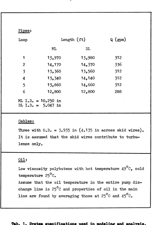
initialization of rapid oil circulation at the peak load periods. The flow rates needed for the forced cooling operation were determined from the desired cable loading and the cable-to-oil heat transfer
Pipes: Loop Length (ft) Q (gpm) ELT DL 1 13,970 13,980 312 2 14,170 14,370 336 3 13,360 13,560 312
4
13,340
14,140
312
5 13,860 14,660 312 6 12,800 12,800 288 ML I.D. = 10.250 in DL I.D. = 5.047 in Cables:Three with O.D. = 3.935 in (4.135 in across skid wires). It is assumed that the skid wires contribute to turbu-lence only.
Oil:
Low viscosity polybutene with hot temperature 490°C, cold temperature 25°C.
Assume that the oil temperature in the entire pump dis-charge line is 250°C and properties of oil in the main line are found by averaging those at 250°C and 45°C.
considerations1 5 and are listed in Tab. 1. Under normal operating conditions ( 300 gpm) the flow would be in the turbulent regime but it could become laminar if the flow rate is significantly reduced, especially in the main cable line.
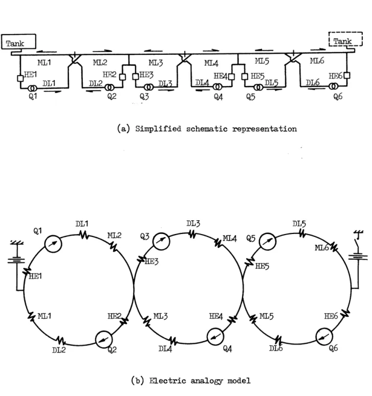
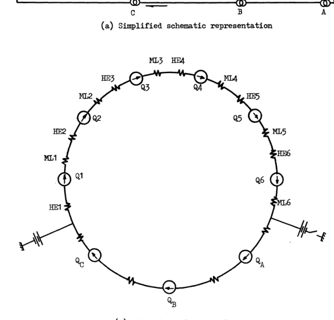
In order ot overcome the flow resistance and provide ample cable cooling during the forced cooling operation, the feeder has to be divided into smaller segments. As shown in Fig. la or 2a, there are six loops, each provided with a pump station and a heat exchanger. The heat exchangers are located upstream from each pump since they are much easier to manufacture for lower pressures. The flow direction in each loop is opposite from its neighbor's as in-dicated on Fig. la or 2a. Since there are pressure control head tanks at the line ends only, if an imbalance occurs in one of the loops, the imbalance can propagate in the direction away from the head tank. This imbalance propagation is discussed in greater detail in Chap. 5. The system specifications pertaining to the planned forced cooling operation are listed in Tab. 1.
3. SURVEY OF POSSIBLE SOLUTIONS
The purpose of this study was to find a system configuration and its pressure profile control which, with imbalances in the system, would maintain constant, or, at least, maximize the main cable line
(ML) flow rates. Imbalance effects on the system should be minimal and the pressure control scheme should be easy to implement with limited adverse effects on the system.
This chapter contains a brief description of various design ideas (system configurations and line pressure control schemes), some of them perhaps impractical, and the merits of individual ideas are evaluated and compared. The feasible solutions are selected for closer analysis and evaluation in Chap. 5.
Following design limitations were observed:
The feeder has to be divided into smaller segments. The length of each segment is selected according to available sites for pump-ing and refrigeration stations and on the basis of the pumps capacity and their pressure rating. As discussed in Chap. 8, to improve the system controllability the segment lengths may vary.
Due to the relatively low pothead strength ( 400 psi), the flow direction in the terminal loops should always be toward the potheads and not away from them, so that the pressure drop across the main cable line of the last segment would reduce the pothead pressure.
For obvious reasons it is not practical to build pressure control head tanks (HT) along the entire cable route. A head tank on each end of the line should be built. The operating HT pressure is governed by the route profile and the oil demand considerations. The upper limit of the HT pressure (400 psi) is determined by the strength of the potheads and the pipes. The lower limit is deter-mined by ionization tests of the cooling oil6 and by the existing
line pressure profile. Nowhere in the ML of the system should the pressure be allowed to drop below the oil breakdown pressure when the
oil begins to lose its insulation properties. As a safety measure, when using the oil whose properties are listed in Tab. 1, a 4
pres-3
sure should never be allowed to drop below 150 psia3.
Each pump must be provided with a relief valve, protecting it from excessive differential pressures. With the gear pumps to be used on the Dunwoodie - Rainey installation the pump pressure rating
is approximately 450 psi. If a constant pressure source (relief valve maintains constant pump head H) is not used, to maintain a pump
dis-charge pressure below the pipe strength limit (here about 800 psia), additional pump control, independent of the pump head control, must be provided. Either the pump inlet or the pump discharge pressures can be followed to determine the instant at which the pump discharge pressure control should begin. For this purpose either the HT pres-sure adjustment, pump bypass, pump shutdown, or one of the artificial
blockage type imbalance controls, discussed in Sec. 3.2 and Chap. 6, can be used. The selection of a method should be such, so as to limit its effect on the system, in a sense that it should cause the smallest possible reduction of the ML flow. For this reason a pump shutdown should be avoided. It should be used only in cases when other schemes fail to provide sufficient amount of control.
3.1. System Configurations
3.1.1. Configuration 1
This configuration corresponds to that of the present Dunwoodie -Rainey installation, and is described in the first paragraph of
Chap. 2. Fig. 1 represents this configuration with constant pressure sources and Fig. 2 is Configuration 1 with constant flow sources.
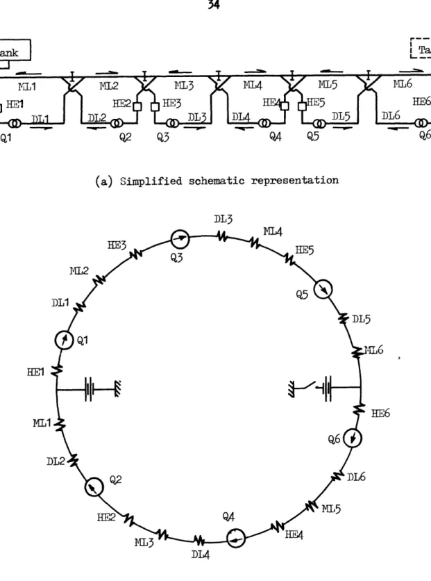
3.1.2. Configuration 2
Shown in Fig. 3, this configuration requires flow blocking diaphragms placed in the ML at locations where the discharge lines (DL) of all unit loops are connected to the M. The DL connections are crossed and thus circuits formed of two units each are created. A unit loop in the Configuration 1 is equivalent to a circuit in
kO wD 0 4, 4, $40 -Pa) 0w
a)
v Fq a) FA 0 .,A 4-) n 0 Id C. 4 H ,I C\JCRi%.
U) $4 ,.l~~~~~a 0~~ U)a rd U 0 H 0~~ a ) t H~~~ C',~ ~
T $4~4
oI Ft 4,b24,~~~~~~F
02 0 *ri02 0 Cd @ *d C0 C) > h~~~~00
0
4=I
HI
00 -40
d H C 0C) 00
Is~~~~~~c
to ~ ~ ~ ~ *d *,r
h
Ou 0 P.14 02 CM - 0o . 0 CT
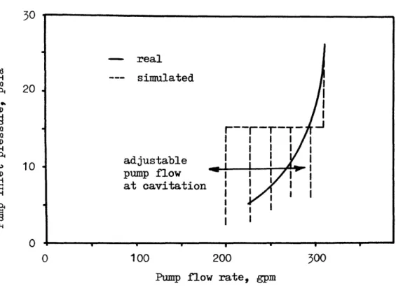
15 4 0 p4 Cd 0co 0 1-4 4) a) at 0 C) o ,1 .V02 rd 0 --I CM IH P4 0 C2Q1 Q2 Q3 Q Q5
(a) Simplified schematic representation
(b) Electric analogy model
Fig. 3. Configuration 2 with pump relief valve arrangement as constant flow sources.
this configuration. This concept will prove to be useful in the treatment of imbalances in Chap. 6.
3.1.3. Configuration 3 (Fig. 4)
The flow blocking diaphragms are located between each pair of the unit loops and all pipes joining the ML are crossed so that a single circuit is formed. For this reason the flow rates are iden-tical everywhere as is apparent from Fig. 4b.
3.1.4. Configuration 4 (Fig. 5)
~he liquid is pumped in one direction along the ML and is sent back through the return line by additional pumps. The flow blocking diaphragms are placed across each ML pump and must therefore be capable of withstanding a pressure equal to the maximum pressure rating of these pumps (here 450 psi). Since the distance between the pump stations is determined by the cable cooling requirements, the ML pump separation and their capacity must be the same as in the Con-figurations 1, 2, and 3, but, due to the absence of long discharge lines (needed in Configurations 1, 2, and 3), the ML pumps load is smaller and so their pressure rating can also be much smaller than the pressure rating of pumps in Configurations 1, 2, and 3.
Q1 Q- 2 Q3 - Q4 Q5 - - Q6
(a) Simplified schematic representation
DL3
HE1
ML
D4
(b) Electric analogy model
C B A (a) Simplified schematic representation
NL3 HE4
(b) Electric analogy model
3.1.5. Conclusion
The advantage of the Configuration 1 over the other configu-rations is the fact, that for its operation it does not require the use of the flow blocking diaphragms. Another argument against the use of Configurations 2, 3, and 4 is the possibility of forming of hot spots in the diaphragm neighborhood.
In the Configuration 4 the flow direction is away from one of the potheads and the pressure on this pothead may, for some imbalances, exceed the pothead strength. This could be used as a major argument against the application of this configuration.
3.2. Line Pressure Profile Control
Since there can be pressure control head tanks (HT) at the line ends only, any imbalance can affect the pressure profile and the flow rates of the entire system. An ideal line pressure profile control
should maintain all system pressures within their specified limits with no further reduction of flow due to the control application. For
the present six loop Dunwoodie - Rainey system the pressure limits are presented in Chap. 2 and for convenience again here:
Max. pump discharge pressure P2 max = 800 psia
Ilax. pump head H = 450 psi
max
Min. pump inlet pressure P = 15.3 psia cay
Max. main line pressure P3 max = 600 psia Min. main line pressure P4 in = 150 psia
P4 nan = 150pi
The determination of P is discussed in Sec. 4.1.1. cay
In this section various line pressure profile control pos-sibilities are presented. Except in the case of the head tank pres-sure adjustment, only the control effects on the loop in which the control is applied are discussed here; the more complex control ef-fects on the rest of the system are discussed in Chap. 5, Chap. 6, and in the Appendix B and the presentation there is limited to the viable solutions only.
3.2.1. Pump Pressure Relief Valve As the Pump Discharge and Inlet Pressure Control
(a) Pump and its relief valve as a constant pressure source:
The pump relief valve is adjusted for the desired ML flow rate and the resulting pump head is thereafter maintained constant by fur-ther proportional opening or closing of the relief valve. Thus, if the absolute pressure level of a loop is controlled by some other means, such as the HT pressure adjustment discussed in Sec. 3.2.2, the relief valve can simultaneously control the pump head and pump discharge pressures.
The disadvantage is the relatively large DM flow reduction when a blockage type imbalance occures as compared to a constant flow source of the following section. Much of the pump power is wasted since the gear (positive displacement) pump continues to supply the same amount of flow, a large portion of which has to be bypassed and is not used for cable cooling. This could be somewhat corrected by using a centrifugal pumps (constant head), but the large ]EL flow rate reduction would still be realized when a blockage occurs. This system will be shown in Chap. 5 to be inferior to the constant flow source
system.
(b) Pump and its relief valve as a constant flow source:
In this method the pump pressure relief valve is initially adjusted for the proper main cable line (ML) flow rate. Further
opening of the relief valve is delayed until the pump head reaches its specified maximum value (here ^ 450 psi) and then the valve maintains the pump pressure head constant. The flow rate is
main-tained almost constant; some flow reduction is observed when larger blockage develops in the line. Since the relief valve controls the pump differential pressure only, additional control on the pressure level must be provided (just as in the case of the constant pres-sure source) to protect the pipes from overprespres-sure. Any of the
imbalance controls, such as the HT pressure adjustment, pump bypass, pump shutdown, or an artificial blockage can be used as the pressure level control.
3.2.2. Head Tank Pressure Adjustment As the Total Line Pressure Profile Control
With this method alone, the pressure profile can be moved up or down. The method consists af varying the head tank pressure according to the behavior of the line pressure profile. The control can be applied continuously (proportionally to the highest or low-est absolute pressure along the line) or only at instances when a line pressure is outside its limits.
(a) Single pressure control (SPC):
The pressure at one end of the line is controlled by a HT and the pressure at the other end is allowed to freely vary accor-ding to the conditions existing within the system.
The implementation of this method consists of the observation of the inlet and discharge pressure of all pumps along the cable route. When one or more of the pressures deviates from its limits, a new HT pressure is determined in such a way that all the pump inlet
and discharge pressures remain within their limits. If this is not possible, that is if an inlet pressure and a discharge pressure are both simultaneously outside their limits (one too low and the other too high), an additional control may be necessary. Either the pump bypass or pump shutdown may be used for this purpose.
(b) Transverse flow dual pressure control (DPC):
Pressures at both ends of the line are controlled by simul-taneous operation of the head tanks located on both ends of the line. In this method of imbalance correction, a return line has to be built, or some other means of transferring the oil between the two head tanks must be provided
The advantage of this scheme is the fact that pressure devi-ations from the normal operating conditions (NOC) due to imbalances are generally lower than in the non-transverse flow schemes, such as the SPC, with comparable imbalance sizes (see Chap. 5 and Fig. 16). At the same time, however, some L flow rates are reduced and some increased by the amount of the transverse flow. This flow reduction coupled with the requirement for a return line are the major disad-vantages of this method.
(c) Non-transverse flow dual pressure control:
As in (b) both head tanks are operated simultaneously, but as soon as the oil starts to flow from or into a HT, the flow is stopped by changing either HT pressure setting. As in (a) the normal HT pressure setting is determined by monitoring all pump pressures and keeping them within their limits. This scheme is actually a single pressure control (SPC) of (a) since the same pressure profile and flow rates can be achieved by using only a single HT.
3.2.3. Pump Shutdown As Emergency Pump Discharge Pressure Control
Either the pump inlet or the pump discharge pressure can be used as the control input to determine the instant at which the pump shutdown should be initialized. When a constant pressure sources are used, the two alternatives are equivalent, but in constant flow source systems they are not ( see next section and Chap. 5).
(a) Pump inlet pressure as the control input:
In this method, when a pump inlet pressure exceeds a set limit, the pump is shut down. The pressure for which the control is set is equal to the maximum allowable pump discharge pressure P2 ma minus
the maximum allowable pump head Ha x (here P2 ma- Hma = 800
-450 = 350 psia).
The major drawback of this method is the fact that in constant flow source systems, when the inlet pressure exceeds a set limit, the discharge pressure may still be safely far from its limit. This situation may be worsened if the ML pipe pressure rating is lower than the pressure rating of DL pipe. Then,in order to assure, that a ML does not exceed its upper limit, the maximum allowable pump
discharge pressure must be lowered (a situation like this will exist on the Dunwoodie - Rainey system since the maximum ML pressure there is 600 psia - 200 psi less than the DL pipe pressure rating). A treatment of this possibility is presented in Sec. 5.3. The reason for the difference between the inlet pressure observation and the discharge pressure observation for the purpose of the pump shutdown is the fact that the imbalance raising the inlet and discharge pres-sures has originated outside the loop in consideration and could not therefore increase the differential pressure.
(b) Pump discharge pressure as the control input:
The control in this method is applied directly by measuring the pump discharge pressure. It permits continuous pump operation in situations where the pump inlet pressure observation in constant
flow source systems would already call for the pump shutdown. A disadvantage lies in the fact that if a pump shutdown is necessary, the resulting discharge pressure fall, which must follow, would cause the pump to be turned on again and thus chattering would ensue. Ther are several ways to cope with this phenomenon:
(aa) anual pump start-up:
At the moment of a pump shutdown, the control is discontinued and an operator has to determine, by observing the pump inlet pres-sure, whether he could turn on the pump again, and would do so manu-ally. The manual pump start-up would be coupled with the reinitia-lization of the automatic pump shutdown.
(bb) Inlet pressure controlled pump start-up:
As a pump is shut down, the control input is switched from the pump discharge pressure to the pump inlet pressure. Thus, the possibility of chattering would be removed, since after a pump is shut down its inlet pressure rises, rather than decreases as does the pump discharge pressure. The automatic pump start-up would be coupled with switching the control input from the pump inlet pressure back to the pump discharge pressure.
3.2.4. Pump Bypass As the Pump Discharge And Inlet Pressure Control
This line pressure profile control is an alternative to the head tank pressure adjustment or the pump shutdown and is best suit-able for application on systems with constant flow sources. It can also be usedas a secondary control to back-up the HT pressure adjust-ment control.
A combination of a pump bypass and a constant flow source creates a component, which, during normal operation, has a constant flow source characteristics, but which, when the bypass opens to cor-rect a pump pressure, has a flow - pump head characteristic equal to a constant pressure source.
The pump bypass can be implemented by further opening the pump pressure relief valve, or by providing the pump with an addi-tional bypass pipe and a valve. The valve control for the pump dis-charge pressure control can be based on either the pump disdis-charge or inlet pressure, just as the pump shutdown was in Sec. 3.2. with similar consequences. Obviously, using the pump discharge pressure as the bypass valve control input is the better alternative, since the pump head is not, in general, constant.
The valve control for the pump inlet pressure control should be based on the pump inlet pressure since, again, the pump head is not constant in the constant flow source systems.
Thus the bypass valve opens when the pump inlet pressure falls below a set limt (here 130 psia - Sec. 5.3), or when the pump dis-charge pressure exceeds its set limit (here 700 psia - Sec. 53). This dual function of a bypass valve is possible because reduction of flow around the loop simultaneously raises the pump inlet pressure and lowers the pump discharge pressure.
3.2.5. Artificial Line Blockages As the Pump Discharge And Inlet Pressure Control
Even though obviously impractical, this method is presented here in order to demonstrate all possible pressure control solutions. A natural line blockage has the same effect as an artificial one and thus the following can also be viewed as a description of the Configu-ration 1 response to various natural line blockages.
Flow limiting valves placed at a pump inlet or discharge line or even a ML can alter the pump inlet and discharge pressures. If the pressure at one of the ends of the ML is kept constant, the effect of closing down such a valve is the same as a line blockage would have on the loop.
In a loop with a constant pressure source (see Sec. 3.2.2) closing down a pump inlet valve (or HE blockage) will reduce both
whereas in a loop with a constant flow source (Sec. 3.2.3), where the pump head H is allowed to increase, the discharge pressure will be reduced less than the inlet pressureand the T flow rate will be reduced less than it would with a constant pressure source.
Closing down a pump discharge valve (or DL blockage) in a loop with a constant pressure source will increase both the inlet and dis-charge pressures equally, and reduce the ML flow rate. In a loop with a flow source the discharge pressure will be increased more than
the inlet pressure and the l flow rate will be reduced less than it would, had a constant pressure source been used.
The effect of closing down a valve in the IM (or ML blockage) depends on which ML pressure is kept constant. In any case the ML flow rate will be reduced, and more so if a constant pressure source is used. If P3 (pressure at the point between ML and DL) is not al-lowed to vary, then in a loop with a constant pressure source closing down a ML valve will equally reduce the inlet and discharge pressures, and with a constant flow source, since H is allowed to increase, the inlet pressure drop is larger than the discharge pressure drop. If P4 (pressure at the point between ML and HE) is constant, then in a loop with a constant pressure source closing a ML valve will equally increase the inlet and discharge pressures, and with a flow source the discharge pressure increase will be larger than the increase of the in-let pressure.
3.2.6. Conclusion
The effects of pump shutdown, bypass, and line blockage out-side the loop of their origin depends on the number of operational head tanks and their location. These effects are discussed in Chap. 5 and illustrated in the figures of Chap. 5 and Appendix B.
It is apparent that both the constant pressure sources and the constant flow sources are possible pump configurations. Of the HT pressure adjustment methods only the single pressure control (PC)
is a viable solution. For the pump bypass or shutdown the discharge pressure observation is the method to be used. When a pump is shut-down, to prevent chattering, the (aa) method of manual pump start-up seems to be the simplest solution. All these mentioned methods of the line pressure profile control are further analyzed and evaluated in
4. STEADY STATE SIMULATION BY THE ELECTRIC ANALOGY METHOD
In order ot simplify the search for new configurations and pressure profile control schemes, and to ease the steady state analy-sis of the more complicated systems, it was decided to build an
electric analogy model.
4.1. Comparison of Prototype and Model Functional Relationships
Two fundamental analogies exist between the performance of an incompressible fluid in a pipeling network and of electricity in a resistive circuit. With electric current representing flow, the total current approaching a terminal equals the total current leav-ing it, just as fluid flows balance at a pipeline junction. With voltage drop representing friction head loss, the voltage drop around a closed circuit is equal to zero just as fluid head losses balance around a pipeline loop.
If an electric circuit is connected to simulate a pipeline network, and suitable conversion factors ae used to relate electric and hydraulic quantities, the performance of the pipeline network is indicated by conditions in the electric circuit. Complete proportio-nality of corresponding quantities does not occur, however, unless
related to the current through it in a manner analogous to the non-linear relation of turbulent flow between head loss and flow rate for the pipeline that it represents. Two general methods have been deve-loped7 previously for satisfying this nonlinear relation. The first is a direct analogy that involves one or more succesive approximations, between which the settings of ordinary linear resistors must be changed in the direction indicated by the preceding trial, the second method consists of the analysis of pipeline networks by means of electric circuits whose resistors automatically represent an accepted relation between head loss and flow rate in the turbulent regime. The posi-tive variation of resistivity of tungsten with temperature, and there-fore with resistor current, is employed in the nonlinear resistors used in the later method. Excellent correspondence between the
hydra-7
ulic and the electric systems was obtained by both methods7 . A model utilizing nonlinear resistors, however, is relatively expensive and complicated for the use in this work. Also tungsten resistors are not easily available.
It was decided therefore to use a different approach from the two methods just described. The following presentation describes the electric analogy model used in the analysis of a six loop pipeline network with its basic configuration corresponding to Fig. 2 with the pump-relief valve arrangement corresponding to a constant flow source
the model, linear resistors were used throughout since in a linear system the effects of individual imbalances can be superimposed on each other and since such a model is inexpensive and relatively easy to build and operate. No iteration or succesive approximations are necessary. After the collection of data, this method involves com-putations for corrections of the results as shown in the Appendix A. Since, however, the qualitative analysis is more important here than the actual numerical results, no corrections were applied to the data presented in the figures of Chap. 5 and the Appendix B.
4.1.1. Characteristics of Positive Displacement Pumps '4
'1 7 1 9
It is assumed that identical gear pumps are used in each loop. Since the length of each ML segment is different, it is necessary to provide the pumps with a special bypass to obtain the required flow rates. It is also assumed that the unit with the largest flow rate would govern the pump selection, and would not be provided with a bypass. The maximum pump head is given as 450 psi and the maximum discharge pressure is 800 psia; the volumetric efficiency of a typi-cal gear pump without the special bypass is approximately 90%o and the pressure drop across the HE in the unit with the largest given flow rate (which is i',2) is set at 40 psi.
displa-cement pumps at steady state. The delivery of a pump can be divided into three factors:
Q Q 0 o - <, -
r
(4-1)The ideal pump delivery Qo0 = Q / v is a function of the pump
phy-sical dimensions and its shaft speed:
= ab (4-2)
The leakage is caused by the flow through the small clearence spaces between the various parts that separate high and low pressure regions, and here, considering the pump special bypass to be a part of the pump, the bypassed flow is an additional source of leakage. The cavitation losses become significant when the pump inlet
pres-sure approaches the pumping liquid vapor prespres-sure.
An exact pump model is a current source in parallel with a resistor, representing the pump leakage. In general, the leakage resistance is nonlinear (turbulent flow through the bypass, laminar flow through the small clearence spaces), but here, since a linear model is being built, the leak resistance must be linearized. Using the Ohm's law:
where H is the pump pressure head and r' is the linearized leak resistance.
Knowing the pump volumetric efficiency without the special bypass, v ', the pump head (from Tab. 2) and the actual desired NML flow rate under OC (normal operating conditions) Q, the linear
leak resistance r' for each pump can be determined from (4-3) and from:
= o Q -2 v - % (4-4)
since it is assumed that the flow rate of pump 7,2 would be equal to the required ML2 flow rate and therefore the leakage of pump 2 would be due to the flow through the small clearence spaces of the pump only.
Thus
r
= H /Q
= H / ( - Q) (4-5)and the values of r' for each loop are listed in Tab. 3.
The appearence of cavitation usually is evidenced by the drop in pump head and efficiency below the well established values under ample net positive suction head (NPSH) conditions10'1 2'1 3 NPSH is defined as the absolute suction pressure less the vapor pressure at suction temperature. Since it is known that in the case of mixtures
of oils the required NPSH is lower and cavitation less severe than in the case of cold water , the cold water NPSH at cavitation in-ception is a good approximation for limiting NPSH. Since oils have generally lower vapor pressures than cold water, assume that the in-let oil pressure at which cavitation begins is the pressure corres-ponding to cavitation with water:
p
= NPSH
+
cav water water vapor atm
= 0.1722 +
0.3887
+14.696
(4-6)
= 15.257 psia
It can be therefore safely assumed that cavitation will not occur when
Pca 15.3 psia cay
The cavitation model consists of a variable resistor and a switch relay connected in parallel between the pump and the circuit. When the inlet pressure drops below 15.3 psia the switch is closed and the flow and pump head reduced. The actual pump cavitation per-formance is compared with the model perper-formance in Fig. 6.
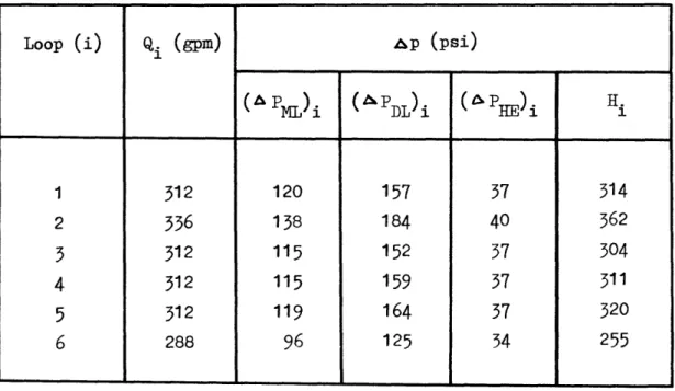
The pump relief valve is modeled by a zener diode connected across the pump. The flow through such a diode is virtually zero
0 100 200 300 Pump flow rate, gpm
Fig. 6. Comparison of the pump cavitation performance with the simulated performance.
pump runs continuously m7I ? oil tank relief valve i ,, U .1Loop #1
Fig. 7. Head tank system used on the Dunwoodie -Rainey installation. 20 10
.,,
0 A 0M 0 0 H $1 - real --- simulated adjustable pump flow at cavitationI
0r
t
_-! I _ I-UU----until the pump head (voltage across the zener diode) equals the diode face value. Then the pump head remains constant and all additional flow is directed through the diode. The diode face value is equal
to the maximum allowable pump head H divided by the conversion max
factor m (Sec. 4.2).
4.1.2. Pipe Flow At Steady State9'1 1'1 5
It is known that pressure changes along a pipe in steady, fully developed turbulent flow functionally depend on the Reynolds number and the relative roughness of the pipe. This unknown funo-tion is in practice known as the fricfuno-tion factor f. The fricfuno-tion factor is defined by:
f=
p /
( 2 L v
2/ d)
(4-7)
For flow in circular pipes the Moody diagran (e.g. Ref. 11) can be used to determine f as a function of the Reynolds number. For the flow in pipe type cable systems an f versus Re correlation was ob-o
15
tained by Slutz et. al. 5 Given the flow rate, the pressure drops are found from (4-7) and listed in Tab. 2 :
p a q2 = a = 2 L / d A2 (4-8)
Table 2. Calculated pressure drops using specifications of Tab. 1.
Loop (i)
Qi
(gpm)Ap
(psi)( PL)i ( PDL)
i ( PHE)
i
Hi
1 312 120 157 37 314 2 336 138 184 40 362 3 312 115 152 37 304 4 312 115 159 37 311 5 312 119 164 37 320 6 288 96 125 34 255A simple linear approximation gives:
Ap =a' q' a' =
a
Q(4-9)
where a = nonlinear pipe flow resistance a'= linearized pipe flow resistance
L = pipe length
A = effective pipe cross-sectional area d = equivalent pipe diameter
v = flow velocity
q = fluid flow rate associated with a
q= fluid flow rate associated with a' = fluid density
4.1.3. Head Tank Modeling
The head tank system consists of a pump which continuously sends pressurized oil from a reservoir through a valve back to the reservoir3, and is sketched in Fig. 7. The valve is set for pressure needed for satisfactory system operation and this pressure is further called the HT pressure. When transverse flow from a HT exceeds the pump capacity, the HT pressure begins to drop. The model maintains a set pressure and the pressure drop due to the transverse flow is
simulated manually.
4.1.4. Elevation Modeling
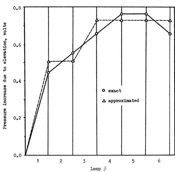
The increase of pressure level due to elevation was taken into account in a lumped model form in loops #1 and #3. The exact and approximated pressure increase due to elevati n are compared in
Fig. 8.
4.2. Electronic Components And Circuits Used In Modeling
The availability of electric and electronic components
governed the selection of the scale factors relating voltage to pres-sure and current to flow rate. These factors are:
m = 165 psi / volt n = 6.1 gpm / a
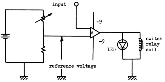
Operational amplifiers were used extensively to operate the switch relays used for pump shutdown and in the cavitation model, and to provide lossless voltage outputs. A voltage comparator circuit is shown in Fig. 9. The absolute value of the output vol-tage of such a circuit is constant, but the volvol-tage polarity
abrupt-Va V
1 2 3 4 5 6
Loop #
Fig. 8. Comparison of the exact and approximated pressure increase due to elevation.
0.8 w 4, H O ,m 0.6 0
0.2
4N
0 rd,0.4
0 0 -H C) 0.2'I
c'rFig. 9. Voltage comparator circuit.
in
Fig. 10. Voltage follower circuit.
switch relay coil
ly changes when the input voltage reaches a reference voltage. The operational amplifier output connected to a switch relay will then close or open the relay depending upon the operational amplifier input voltage. A voltage follower circuit is shown in Fig. 10. The output voltage of such a circuit is equal to its input, but the cir-cuit draws a negligible amount of current (- 10-9amps).
4.2.1. Pipeline Network Modeling
Linear variable resistors were used to represent each pipe aegment, with the minimum resistance equal to that existing in the prototype under NOC. Using the pressure drop values of Tab. 2 and Eq. (4-9), the NOC flow resistance values were found and are listed
in Tab. 3, after being multiplied by the factor of n/m, and after the resistance of the current meters and elevation modeling circuits were taken into account. Increase in pressure due to elevation was
simulated by battery and resistor circuits placed in loops #1 and #3 as shown in Fig. 14.
4.2.2. Pump Modeling (Fig. 11 and Fig. 12)
A flow source and a resistor in parallel can equally be rep-resented by a voltage source and the resistor in series, if linear
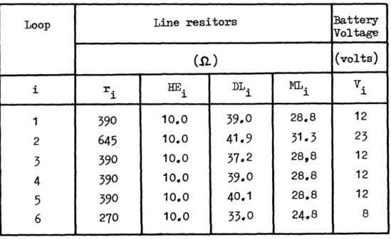
Table 3. Model resistor and battery voltage values.
Loop Line resitors Battery
Voltage .
~
_,. (D2) (volts) i r i HE. DL. ML. V. 1~~ 1 1 1 1 390 10.0 39.0 28.8 122
645
10.0
41.9
31.3
23
3
390
10.0 37.2 28,8 124
390
10.0
39.0
28.8
12
5
390
10.0
40.1
28.8
12
6
270
10.0
33.0
24.8
8
.~~~~~~
"I
1fl
Qo
Fig. 11. Pump modeling.
Relief valve model
V= rt Q
-o
automatic
relationship between pressure drop and flow rate is assumed. Thus the pumps are modeled by batteries and linear resistors in series. The leakage resistor values were found from (4-5) and are listed in Tab. 3, after being multiplied by the factor of n/m. The battery voltage values were found by using the Thevenin theorem:
V = r' Q (4-10)
and are also listed in Tab. 3, after being multiplied by the factor of 1/m
The face value of the zener diodes representing the pump relief valve was found by scaling the value of Hm = 450 psi by
multi-plying it by the factor of 1/m
For the pump shutdown a switch relay was operated by a voltage comparator circuit which utilized either the pump inlet or discharge pressure as its input at the decision of the model operator.
As mentioned in 4.1.1, the pump cavitation was simulated by a variable resistor which could be adjusted for the desired cavitation extent. The resistor was added in series with the battery by the action of a switch relay operated by a voltage comparator circuit based on the pump inlet pressure (Fig. 9)
4.2.3. Head Tank Modeling
The model as shown in Fig. 13 has built-in all of the func-tions of the real HT system shown in Fig. 7 and described in Sec. 4.1.3. For satisfactory HT model performance, the electric current corresponding to the HT pump capacity should be much larger than the minimum current needed to cause a voltage drop across the zener diode to equal to its face value V That is, it should be of the order of 20 - 30 ma. Since the maximum HT pump flow is only about 5 gpm, the conversion factor would have to be of the order of 0.2 gpm / ma. Since the pump flow rates are around 300 gm, the model currents would have to be in the neighborhood of 1.5 amperes, with the need for correspondingly large batteries or power supplies. It was decided therefore, in order to be able to use regular size heavy duty batteries, to keep the current level down at 20 - 30 ma corres-ponding to t NOC flow rate of 300 gpm. Thus the model HT pressure will not drop when the transverse flow reaches the capacity of the HT pump ( 5 gpm). It is very simple, however, to perform this func-tion manually by changing the T pressure setting in such a way so as to maintain the transverse flow at or below 5 gpm.
4.2.4. Voltage Measurements
V z
-Us---Fig. 13. Head tank model
-.
Vel
Fig. 14. Elevation modeling.
'1 Ila
e2
-voltmeters, the voltage follower circuits were utilized as shown in Fig. 10. The voltmeter resolution was 0.02 volts.
4.2.5. Current Measurements
Each ML current was measured by microammeters and their in-ternal resistance was included in the ML resistance. Since the current through the ML's was in the 20 - 30 ma range, the microammeters were connected across shunt resistors and therefore the scale factor n has the units of gpm / a.
-9 +9
. ML
V
z
Fig. 15. Complete model of a unit loop.
+910 M
V
5. EXPERIMENTAL PROGRAM AND RESULTS
Since only the Configuration 1 is applicable today (requires no flow blocking diaphragms for its operation), imbalance effects on this configuration were investigated in &eater detail. An imbalance is defined as a pipe flow blockage or resistance increase, pump flow bypass, or a pump shutdown which alters the pressure profile or the flow rate in the system. The difference between the schemes using single HT (single pressure control - SPC) and two HT's (dual pres-sure control - DPC) is very small, since the HT pump capacity is only 5 gpm. When the pump capacity is increased and transverse flow allowed by building a return line, this difference may become signi-ficant, but from the simulation tests it was discovered that all pressure deviations from NOC due to a practical size blockage would be smaller, but not significantly smaller, in DPC than in SPC, every-thing else being equal. At the same time, the ML flow rate in loops having oposite ML flow direction to the direction of the transverse flow would be reduced by the amount of the transverse flow, whereas in loops with the ML flow direction in the direction of the transverse flow the flow rate would be increased by the same amount. An example is given in Fig. 16 (for better understanding, the reader may find it convenient to postpone the study of this figure until after he finishes reading Sec. 53).