Asymmetric business cycles : theory and time-series evidence

#pe****t

>*

l

UBRAfflBS)

&

Vk

V

Jo

Digitized

by

the

Internet

Archive

in

2011

with

funding

from

Boston

Library

Consortium

Member

Libraries

HB31

!

.M415

working

paper

department

of

economics

DEWEY

)i

ASYMMETRIC

BUSINESS CYCLES:

THEORY

AND

TIME-SERIES

EVIDENCE

Daron

Acemoglu

Andrew

Scott 95-24

Aug. 1995

massachusetts

institute

of

technology

50 memorial

drive

Cambridge,

mass.

02139

ASYMMETRIC

BUSINESS CYCLES:

THEORY

AND

TIME-SERIES

EVIDENCE

Daron

Acemoglu

Andrew

Scott

MASSACHUSETTSINSTITUTE ,

--.•ogy

95-24

ASYMMETRIC

BUSINESS CYCLES:

THEORY AND

TIME-SERIES

EVIDENCE

Daron Acemoglu

Department

of

Economics

Massachusetts

Institute of

Technology

and

Andrew

Scott

Institute of

Economics

and

Statistics

and

AH

Souls College,

Oxford

University

August 1995

JEL

Classification:

E32

Keywords:

Asymmetries,

Cyclical Indicator, Intertemporal Increasing Returns

Regime

Shifts,

Temporal

Agglomeration,

Unobserved Components.

Abstract

We

offera theory of

economic

fluctuationsbased

on

intertemporal increasingreturns: agents

who

have been

active in the past face lower costs of action today. This specification explains the

observed persistence in individual

and

aggregate output fluctuations

even

in the presence of i.i.d shocks, essentially because individuals respond to the

same

shock

differently

depending

on

their

recent past experience.

A

feature of our

model

is that output

growth

follows an

unobserved

components

process with special

emphasis

on

an underlyingcyclical indicator.

The

exactprocess for

output, thesharpness ofturning points

and

thedegree of

asymmetry

aredetermined

by

the

form

that

heterogeneity takes.

We

suggesta generalformulationfor

models

withlatentcyclicalvariableswhich, under certain assumptions, reduces to a

number

of state space

models

that

have been

successfully

usedto

model

U.S.

GNP.

Using

ourgeneralformulation

we

findthatallowingforricher heterogeneity

enables us to obtain a better fit to the data

and

also that U.S. business cycles are asymmetric, with this

asymmetry

manifesting itselfas steep declines into recession.

We

estimate a strongly persistent

cyclical

component

which

is not well

approximated

by

discrete

regime

shifts nor

by

linear models.

Our

estimates ofthe relative size ofintertemporal returns

needed

to explain U.S.

GNP

vary but

on

the

whole

are notimplausibly large.

We

oweaspecialdebttoJamesHamiltonwhoseinsightfulcommentsimproved anearlierversionofthispaper.

We

alsothank

PhilippeAghion, Charlie Bean, RicardoCaballero, PaulDavid, Steve Durlauf, Vittorio Grilli, Christopher Harris, Rebecca

Henderson, Per Krusell, Jim Malcomson, John Moore, Chris Pissarides, Danny Quah, Kevin Roberts, Donald Robertson, variousseminarparticipantsandtwoanonymousrefereesforusefulcomments.Remainingerrorsare theauthors'responsibility.

1. Introduction

Aggregate economic

fluctuations are characterized

by

successive periods of high

growth

followed

by

consecutive periods of

low

activity.

The

transitions

between

these periods ofhigh

and

low growth

areoften

marked

by

sharpturning points

and

considerable evidencesuggests thatatthese

moments

the stochastic properties ofthe

economy

change

and

display asymmetries, see inter alia,

Neftci (1984),

Diebold and

Rudebusch

(1989),

Hamilton

(1989)

and

Acemoglu

and

Scott (1994).

The

importance oftracking these

movements

inthebusinesscycleisreflectedintheconsiderableattention paid to a variety ofcoincident

and

leading indicators (e.g. Stock

and

Watson

(1989),

and

the papers in Lahiri

and

Moore

(1991)).

A

natural

way

to

model

temporal agglomeration1

and asymmetries

in

economic

fluctuations is to

assume

non-convexities, such as discrete choice or fixed costs at the individual level, because such non-convexities

imply

thatindividualsconcentrate their activity in a particular period. It is this

implication

which

has

been

analyzed with considerablesuccess in the(S,s) literature.

However,

while

thepresence of fixed costs can account for the discreetness of

economic

turning points, it does not

naturally leadto persistence -

once

an individual undertakes an action they are less likely to

do

so

in the near future.

The

key

reason is that although the presence offixed costs leads to increasing

returns, these are infratemporal; the full extentof

economies

ofscale arising

from

fixed costs can be

exploited within a period2.

As

a

consequence

persistence in aggregate fluctuations relies

on

aggregation across heterogeneous agents: either

more

agents investing in the past increases the

profitability of investment for others (e.g.

Durlauf

(1991)

and

(1993)) or aggregate shocks affect

agents differently, leading to a

smoothed

response over time (e.g. Caballero

and Engel

(1991)).

This paper

emphasizes

analternativeexplanationofpersistentindividual

and

aggregate output

fluctuations

by

suggesting that fixed costs introduce intertemporal increasing returns, that is, the returns

from

an activity thisperiodare higheriftheactivityoccurredlastperiod

and

asa

consequence

an agent

who

was

active in the recentpast is

more

likely to be active

now.

In the presence of such

intertemporal linkages temporal agglomeration arises

from two

sources; active agents maintaining a

high/low activity level in successive periods because ofintertemporal increasing returns

and

agents acting together, either inresponseto a

common

shock

orbecause ofstrategic complementarities.

We

show

how

a

model

of the

former

explains a

number

of empirical features of business cycle

fluctuations

and

also offer a

framework which

enables an

economic

interpretation of

unobserved

component

models

of U.S. output

which emphasize

the underlying cyclical indicator.

The

relevance ofintertemporal increasing returns

depends

on

(i)

whether

individual behavior ispersistent

and

(ii)

whether

firm'stechnology

and

costs containimportantintertemporal aspects.

The

1

We

use thisterm, following Hall (1991), for thebunching ofhigh economicactivity overtime.

2

To

overcome this problem empirical implementations of (S,s) models sometimes include time-to-build considerations or decreasingreturns at highlevelsofinvestment, e.g.Caballero and Engel (1994).

answer

to these questions will vary

depending

upon

the type of activity

under

consideration. For instance, in the case ofradical changes in the capital stock, e.g.

Cooper

and

Haltiwanger's (1993) automobile retooling, intertemporal effects are unlikely to be important,

and

this is supported

by

the

lack of persistence in these cases.

However,

Section 2 surveys

micro

evidence that firm level investmentis persistent

and

findings

from

technology studies,the

management

scienceliterature

and

organizational theory

which

supports the notion that

many

important discrete decisions (e.g. investment in

new

technology, product development, innovation, maintenance) exhibit

some

degree ofintertemporal increasingreturns.

These

empirical findingsmotivatethetheoretical

model

of Section

3 in

which

a firm has to decide each period

whether

to undertakeboth

maintenance

and

investment.

Maintenance

is

modelled

as having

two

effects: (i) increasing the productivity of existing technologies

and

(ii)facilitating theadoption of

new

innovations.

The

interaction ofthese

two

roles

leads to intertemporal increasing returns: firms find it profitable to maintain the

newly

adopted

technologies

and

this in turn reducesthe costs of adoptingfutureinnovations.

As

aresult, investment

costs are lower

when

the firm has invested last period,

and

a natural

asymmetry

is introduced in

individual behavior; inresponse toa range ofshocks, the agents will finditprofitable to investonly ifthey

have

invested inthe recent past.

Section

4

examines

the aggregate

economic

fluctuations implied

by

individual level

intertemporal increasing returns,

and

illustrates

how

our

model

accounts for the

main

features of temporal agglomeration

and asymmetric

fluctuations: the significance

and

persistence ofa cyclical

component

in output fluctuations,

and

the importance of turning points

and

business cycle

asymmetries.

An

importantfeature of our

model

is itstractability.

Not

only can

we

characterize

how

the persistence of business cycles

and

the sharpness of turning points are determined but

we

also

make

directcontact witha

number

ofeconometric studies

which

rely

upon

an

unobserved

component

model

of output growth, e.g.

Harvey

(1985),

Watson

(1986), Clark (1987). This generality enables

us to nest a variety ofdifferent types ofbusiness cycle asymmetries.

And

this

theme

is

pursued

in

Section 5 where, in the context of our model,

we

examine

the circumstances

under

which

turning points

between

booms

and

recessions are

most marked,

sothatoutput

growth

approximates ashifting

regime

process as in the discrete state

Markov model

popularized

by

Hamilton

(1989). In all these exercises,

we

findthatthe

form

ofheterogeneity (thedistributionofidiosyncratic shocks)is the

main

determinant ofthe time-series properties,

and

also ofthe

asymmetric

nature offluctuations.

Section

6

takes our

model

to data. First,

we

look at the connection

between

our theoretical

model and

a

number

of estimated

regime

shift

models

to infer the size of intertemporal increasing returns necessary toexplain U.S. business cycles.

However,

thereal advantage of our formulation is its ability to nest different

unobserved

component

models

withdifferent specifications regarding the

form

of heterogeneity.

We

thus estimate

two

versions of our general

model

on

U.S. data. This

exercise yields a

number

ofinteresting results. First,

we

findthata versionof ourgeneral

model

with normally distributed idiosyncratic shocks does considerably better than the version with uniformly

distributed shocks, but this latter is precisely

what

previous empirical

work

has used. Therefore, our

model

offers an alternativetime-series representation

grounded

in

economic

theory thatoutperforms

a

number

of popular models.

Moreover,

the difference

between

the versions can be heuristically

thought to be the importance of

asymmetry

terms in the version with

normal

shocks. Thus, our

investigation also establishes that U.S. business cycles are

asymmetric

and

illustrates that these

asymmetries manifest themselves

by

sharp

downswings

in

economic

activity

which

cannot be captured

by

linear models.

Since our formulation is derived

from an

underlying

economic

model,

we

also use the estimation results to

make

inferences about the nature ofthe aggregate

economy.

For

instance,

we

find thatthe cyclical

dynamics

of the U.S.

GNP

cannot

be

characterized as discrete shifts

between

differentregimes, which, inourtheoretical

model

impliesthatthe idiosyncratic uncertaintyisplaying an important role in the propagation of

economic

shocks

and

this is also

confirmed

by

the fact that

we

estimate the variance ofidiosyncratic shocks to

be

larger than that of the aggregate shock.

We

also again find that the size of non-convexity implied

by

the estimation result is

modest and

that

overall the

model

provides a

good

fit to the data.

2. Individual Persistence

and

Intertemporal

Increasing

Returns

Our

interest intemporal agglomeration focusesattention

on problems

in

which

fixed costs are

important

and

so agents

have

to

make

a discrete choice about

whether

or not to

perform

a certain

activity.

A

crucial feature of our analysis will be the investigation of

how

an agent's current qualitative choice (i.e.

whether

or not to

perform

a certain activity) influences the

same

decision

tomorrow.

In the standardcase, an activity thatrequiresa fixed costwill

be

bunched

withinaperiod of time, essentially because fixed costs

imply

the existence of infratemporal increasing returns to scale. This observation lies at the heartof (S,s)

models

(e.g. Scarf (1959))

and

implies that a brief

period ofactivity is followed

by

periods of inactivity at the individual level.

However,

while there is considerable evidence supporting (S,s)

models

(e.g. Bertola

and

Caballero (1990), Caballero

and

Engel

(1994),

Doms

and

Dunne

(1994), Cooper, Haltiwanger

and

Power

(1994)), there is also substantialevidence thatfirm levelinvestmentdecisions are characterized

by

significantpersistence.

For

instance, using

UK

firm level data,

Bond

and

Meghir

(1994) find significant autoregressive

effects in investmentbehavior.

They

estimate equations for theinvestment-capital ratio

and

findI/K,

=

a

+

0.856 I,.

1

/K

t.,(l-0.122 It.,/Kt. 1)+pZ,

+

et

where

Z

t is a vector of firm relevant variables

and

e,

is a white noise disturbance. Evaluating the quadratic

term

at its

sample

mean

yields an

AR(1)

coefficient of

around

0.75.

Bond

et al (1994) estimate

AR(1)

and

AR(2)

models

using Belgian,

French,

German

and

UK

firm panel data finding strongly significant investmentlags, with the

sum

oftheautoregressive coefficients

around

0.3.

Even

the evidence in

Doms

and

Dunne

(1994) reveals

that there is significant investment occurring in

most

years of the

sample

for

each

firm

and

that concentrated investment bursts are spread over several years.

These

findings suggest that while

infratemporal

economies

ofscale (lumpiness) are important there

may

also

be

intertemporal linkages

which

can profitably be exploited. This raises the question,

what form

of investment produces these intertemporal linkages?

The

most

obvious

form

ofintertemporal

economies

of scale is learning-by-doing,

whereby

past experiences increase productivity or reduce costs.

More

explicitly, consider the case

where

incorporating

new

knowledge

is a

slow

and

costly process, limiting the degree to

which

productive investments can be undertaken within a period.

However,

the

more

familiaran individual is with the

most

recenttechnology vintages, thecheaperitis to adoptthelatestversion.In contrastan individual not using the

most

recent vintage faces compatibility

problems

when

dealing with the frontier

technology.

The

result will be that only limitedinnovative

moves

aretaken within

each

period, with

cost incentives

making

forward steps

more

likely to

come

from

active agents.

The

idea that

intertemporal linkages

might

lead agents to take a sequence of small investment steps is given

empirical support in studies of technological innovation. In this literature a distinction is

drawn

between

incremental

improvements

ofanexistingtechnology

and

radical

improvements

which

destroy the existing technology

and

start an alternative production or organizational

method,

e.g.

Tushman

and

Anderson's

(1986) "incremental

change"

versus "technological discontinuities".

There

is widespread

agreement

that the less spectacular incremental

changes

account for

most

of the productivity gains (see

Abernathy

(1980),

Myers

and Marquis

(1969)

and

Tushman

and

Anderson

(1986)).

More

importantly for our paper, there is also a consensus that incremental innovations are

more

likely to

come

from

firms

who

have been

active at the earlier stages of product development.

In

Freeman's

(1980, p.168)

words

"the

advance of

scientificresearchis constantlythrowing

up

new

discoveries

and

opening

up

new

technicalpossibilities,

a firm which

isable to

monitor

this

advancing

frontier

by one

means

or another

may

be

one of

thefirst to realize

a

new

possibility".

Arrow

(1974)

and

Nelson

and Winter

(1982) also

emphasize

the advantages possessed

by incumbent

innovators in being able to further

cope

with incremental changes.

For

instance,

Nelson

and Winter

stress the

importance of engineers understanding

new

technologies, suggesting that firms

who

innovate

have

an advantage in doing so again.

Abernathy

(1980, p.70), using evidence

from

industries diverse as automobiles, airlines, semi-conductor

and

light bulb manufacturing, notes that

"Each

ofthe

major

companies seems

to

have

made

more

frequent contributions in

a

particular

area"

suggesting that previousinnovationsinafieldfacilitatefutureinnovations.

One

possibleexplanationofthese findings are fixed effects:

some

firms

may

simply

be

good

at innovating in certain areas.

However,

the industry

wide

work

of Hirsch(1952),

Lieberman

(1984)

and

Bahk

and Gort

(1993)suggeststhat

more

thanjust individual fixed effects is operating. In the remainder ofthis paper

we

shall focus

on

this

form

of investment

and

its implications for aggregate fluctuations.

3. Individual

Behavior

in the

Presence

of

Intertemporal

Increasing

Returns

(i)

The Environment

We

assume

thatagents (orfirms) are risk-neutral

and

forwardlooking,

and

seek to

maximize

their return (either profit or utility).

The

key

decision is

whether

or not to invest in order to benefit

from

technological progress.

More

explicitly, each period a

new

technology

becomes

available. This technology has a stochastic productivity that is revealed at the beginning of the period.

The

agent

decides

whether

to adoptthis technologyor not,for instance

whether

toinstall a

new

software. Ifthe

technology is adopted, the productivity ofthe agentincreases permanently, starting

from

the current

period3.

To

obtain the highest return

from

this innovation,its compatibilitywith existing technologies

needs to be monitored. Inparticular, at the

end

ofthe installation period there is the option to gain additional productivity

from

the innovation

by

maintenance

4 (e.g. fine-tuning).

Under

these

assumptions the firm's output is

y,=>Vr

a

o + (

a

i+M

/>V

a: 2y/(1 -

m

/)

0)

where

a,,, a,

and

o^ are positive parameters

and

s,

and

m, are binary decision variables that equal 1

ifinvestment (s

t)

and maintenance

(n\) are undertaken this period,

and

equal zero

otherwise. If the

new

technology is adopted (s

t=l), the productivity ofthefirm is higherpermanently.

When

there is

no maintenance

effort atthe

end

oftheperiod

(m

t=0), this increase inproductivity is not as large as

it could be (a,-0C2+ut instead ofo^+u,). Deterministic depreciation is denoted

by

Oq (our results are

unchanged

ifdepreciationis avoided

when

m,=l).

We

assume

thatu,isaseriallyuncorrected

random

shock

to the productivityof investment with distributionfunctiondenoted

by

F(.).

Maintenance

costs are

assumed

to be equal to a positive constant,

_y

(i.e.

C

t

m

=y^).

A

distinctivefeature of(1) is that

as in (S,s) models, our focus is

on

decisions that

have

a discrete nature, e.g.

whether

to adopt the recenttechnologyvintage or

whether

tomaintainexistingmachines.

The

discrete natureofthe choice

explains

why

theproductivity

shock

in (1)is multiplicativewiththeinvestmentdecision; productivity

shocks are associated with

one

vintage oftechnology

and

thereforeonly affect output

when

the

new

technology is adopted.

In this model,

maintenance

also has an additional role other than ensuring the

maximum

performance

ofthe latestinnovation.

More

specifically,

we

assume

investment costs are given by:

c

_{r(YrY2™,-i>,}

(2)

where

bothy,

and

y

2 are positive so that

when

equipment

is maintained thefirm's investment costs

nextperiodare lower.

Here

_y

₂ is the extrainvestmentcost incurred

by

a plant

which

didnotmaintain

Time-to-build considerationscaneasilybeincorporatedinthe returnfunction andonly servetochangethetiming ofreturns.

4

last period. In terms of our

computing

example, all existing

bugs

in the

system

need

to be

removed

to ensure the optimal implementation ofthe

new

software, implying that next period the instalment of another

new

program

is less costly. In contrast, if the

computer

is not maintained, technical assistanceis necessary both atthe beginning oftheperiodfor installation (to

remove

bugs)

and

atthe

end

ofthe period (for fine tuning to increase productivity ifso decided).

Each

periodthefirm decides

whether

toinvest(s

t

=0

or 1)

and

also

whether

tomaintain

(m,=0

or 1).

Denoting

the discount factorofthe representative firm

by P and

theper periodreturn

by

r(.),

we

have: r(s lv

jn

lv

;m

tij_

_v

y

ltj _

v

u

_lv)= >'/y-r

a

o + (

a

i+M

/^-

a

^v<

1"

m

^"

_Y

o

m

<v-(YrY2

m

/+;-i>y/+_;

and

the

maximization problem

ofthe firm at time tis:

max

E,{

Jl^r(s

lv

^n

tv

;m

l+j

_^

H

.

v

u

t

^

}

(4)

subject to (1)

and

taking y,.,,

u

t, m,., as given. Inperiodt+j, the statevariables are m,^.,,ut+j, yt+j .,

and

the choice variables are s

I+j

and m,

+j.

Whether

the firm invests in

any

period

depends

on

ut. In contrast, the return to

maintenance

only

depends

on whether

or not investment occurs. If

no

current investment is undertaken, the only

benefit of

maintenance

is the costreduction that it brings in the following periodifinvestment then

occurs. Incontrast, ifthereis current investment, future productivity alsoincreases

by

ctj.

As

aresult

there are three possibilities regarding maintenance: (i)

always

maintain (ii) never maintain, (iii) maintainonly

when

there isinvestment.

Because

we

wish

to

make

maintenance

adecisionofthefirm

rather than a fixed characteristic,

we

concentrate

on

(iii).

To

this

end

we

assume

5

:

Assumption

A:

0Y <

Y

<A_

(5)

H

2 _°

1-/3

The

first inequality can be understood

by

noting that

_Py

2 is the

maximum

benefit

from maintenance

in the absence of current investment: if there is investment next period costs are

lower by

_y

₂,

otherwise there is

no

benefit. Therefore, the first part of the inequality implies

maintenance

is not

Assumption

A

is stronger than

we

require but simpler to understand than the necessary condition,

worthwhilejust toobtain future cost savings. In thepresence ofcurrent investment, the

minimum

gain

from

investment is the present value of the productivity increase

due

to maintenance, (^/(l-P). Consequently the second part of the inequality states that

even

without future cost savings, it is

profitable to maintain ifthere is current investment. Itfollows that

when

(5) holds,

we

can limitour attention to the case

where

the firm only maintains

when

it invests, thus

m

t=s„

and

the per period

return simplifies to:

Kv^iVJ^^

a

i^"Mv^

(6)

where 5

_{=Y +}

Yi

and 5

l

=y

2

-

Assumption

A

therefore enables us to write our

problem

in a

way

which

focuses

on

the intertemporal increasing returns arising

from

the interactive

term

5,s

t+jst+j.,.

More

generally, (6) can

be

interpreted as the period return for a firm

which

benefits

from lower

current

investment costs, ifit invested last period.

Under

this interpretation our

model

captures the idea that

firms

who

are

used

to adapting to a changing

environment

face

lower

costs offurther changes.

(ii)

Optimal

Decision Rules

Using

(6) the

maximization

problem

attimet can bewrittenin a

dynamic

programming

form

with the value function V(.) satisfying: V(y

t

_^

t_

vu)=sup

{/-(^;y/.1

^.

1,u/)+/3£;/

K(y

/.1

-a

0+(a1+v/

>s^^

/+1)} (7) Solving the agent's optimization

problem

we

obtain (proofin the appendix):

Proposition 1:

The

value function

s

_r

\

and

^(y

M

^

_M

,u><V<^

_M

+

<to-i+

te

*/"^<«V w

rVi

(8)

s=0

and

_{Vfy,.^,.^,)^^,-!}

if

K^Qo-to^

is the unique function _{that satisfies (7)} (<|)'s denote constant coefficients).

To

understandthe

dichotomous

natureofthevaluefunction,considerthecase

where

theagent doesnot invest (s

t=0).

The

disturbance

u

tisirrelevant tofutureprofits

and

with

no

investment costs,

itdoes notmatter

whether

thefirm invested/maintainedlastperiod

and

so the valuefunction

depends

only

upon

y,.,.

However,

ifthefirminvests the valuefunction

depends

linearly

upon

_y

t.„ st.j

and u

t.

The

optimal choice of s

t

depends

on whether

the investment shock, u„ is

above

a certain critical

value.

Shocks

below

this value lead to insufficiently high productivity to

be

embodied

in the firm's

technology.

The

critical value

depends on

s

t.,

due

to the intertemporal non-separability in the cost

iff the difference

between

the left

hand

side of (7) evaluated at s,=l

and

is positive.

Using

the

Appendix and

(8), the agent invests iff

(Jg oo <">0

[1-/8

/

^a'xl^o,^

/

dF(u

hl)+

J-

/

WM

^(u,J]

+S

_lVl+r

U,>0

(9) It is this inequality

which

implicitly defines the coefficients co

and

co, in (8) (see

(A3)

in the

Appendix).

The

intuition behind thisexpression is a

good

way

ofillustratingthe

main

featuresof our model.

The

firm is

comparing

the strategy s,=l with s

t

=0

6

. Ifs

t

=l

production increases

by

oc,+utfor

all periods

compared

to s,=0,

which

has a net present value (including costs) of

(i-/?)>

1+u,)-(S

_-SrVi)

(

10

>

Any

further benefits

from

choosing s

t

=l

depend upon

future values of ut.

There

are three

possible cases:

(i) Ifu_t+1

e

(-oo,(0_{-C0i) the agent}will not invest regardless ofs

t

and

there are

no consequences

beyond

(10).

(ii) Ifut+1

e

[cOq-co^cOo) the household's t+1 investment decision

depends

upon

st

.

The

shock

is only favorable

enough

forinvestmentifthehousehold benefits

from

costsavingsarising

from

past

investment i.e. st+1

=l

ifst

=l

and

st+I

=0

otherwise. In this case, investingtoday

means

a difference in

expected discounted value next period of

u° <->o

P

{

dF(u

m

)x{(l-P)\a

+

f

u^dFiu^y^-SJ}

(11)

u -u)[

where

the first integral represents the probability thatut+1

e

[co -cO|,co )

and

the

second

is theexpected value ofu,₊₁ conditional

on

u_t+1

e

[o) -a),,{0 ).Ifbothut+1

and u

t+2 fallin theregion [(%-<»,, co ) this

same

additional benefitaccrues in t+2, suitably discounted. In otherwords, s

t+2 only equals 1

when

st+1=l,

which

in turn will only be the case

when

s

t=l.

As

{ut} is

assumed

an i.i.d

sequence

this additional

benefit att+2 is (1 1) multiplied

by

pProb(co-a>,<u_t+1<a> ).

A

similar logic holds forallfutureperiods

and

summing

over time yields

{1-0

_/

dF(u

_{hl )}} l

x[{p

_/

iF(u

_M)}x{^

+

₅

r

S

}+

J-

_/

u^dFiu,^)]

(12)

Ourresults are unchanged ifm, and s,lie in thecontinuum [0,1] rather than takediscrete values.In this case, if (9) holds as a strict inequality agents choose one corner, s,=l and

m

t=l; if(9) is strictly negative, st

=m

t=0. If(9)

holdsasanequality agentsare indifferentbetween anychoicethathasm,=st.If in thiscase

we

imposethattheagent

chooses s,=m,=l our results holdexactly.

Equation (12) is the net expected value of all future investment projects the firm benefits

from

only ifitinvests today. Ifthe firm does not investattimet,

and

future shocks fall in the region [co -co,,to ), the firm will not invest in the future.

However,

if the firm invests today the

same

sequence of shocks leads the firm to invest

and

reap the benefits given

by

(12).

Thus

there is an important

asymmetry

in the

way

firms

respond

to investment shocks in high

and low

activity states,

and

as a

consequence

the marginal propensity to invest varies

between

these states. This state

dependence

relies entirely

on

0),>0,

which from (A3)

intheappendixisequivalentto8,>0, orinother

words, the presence of intertemporal increasing returns.

(iii)Finally, ifu_t+1

e

[co .°°). the

shock

is so favorable agents invest regardless of

whether

they benefit

from lower

costs.

However,

while investment decisions are the

same

irrespective of

s,.„ costs are not. If s

t

=

1 the cost of choosing st+1

=l

is

lower by

8„

which

has expected present value of(38,(l-F(co )).

The same

benefit accrues att+2, ifboth u,+1

e

[©

-co,,co )

and u

t+2

e

[co ,°°), with

expected value of f3

2

8

1[F(a) )-F(co -co,)][l-F(aj)], with similar expressions holding for t+3, etc.

Summing

over time gives

Wq CO {1-/3

_/

dF(u

t

JY^jdF{u

t

J

(13)

"o-"i "o

This expression represents the reduction in future costs arising

from

current investment

and

again reflects thepersistence in s„ captured

by

the integral

between

(£>

q-(jsx

and

u)

.

The

sum

of(10), (12),

and

(13) is equal to (9)

and

characterizes the optimal decision rule of households.

The

most

important feature ofthedecision rule,

summarized by

(9), is the

dependence

of current actions

on

past decisions.

Due

to intertemporal increasing returns, shocks in the range [co ,co -a>,) lead toinvestment ifreceived

by

an agent

who

has

been

active in the past (s,.,=l) but not

for an agent

who

has not invested at t-1,

making

individual behaviorpersistent.

4. Cyclical Fluctuations in the

Aggregate

Economy

(i) Characterizing

Output

Fluctuations

We

now

turn to the implications of individual level intertemporal increasing returns for aggregate

economic

fluctuations.

We

assume

the

economy

consists of a

continuum

of agents,

normalized to 1, each of

whom

faces the technology described above.

Because

the intertemporal increasing returns are internal to the firm,

we

allow forcorrelation

between

the different investment

decisions (denoted s,' for agenti) ofheterogenous agents

by assuming

the existence ofan aggregate

productivity

shock v

t. Heterogeneity is firstintroduced via an idiosyncratic shock, £,' such that

each

agent receives a

shock

u^Vj+e,'.

We

assume

that £,' is

drawn

from

a

common

distribution function G(.) (with associated density function g(.))

and

that v, is i.i.d with distribution function, H(.),

and

density function, h(.). Finally,

we

assume

£,'is uncorrected

between

individuals

and

overtime.

Both

investment decisions.

The

decisionrule ofthe individual is giveninsection 3

and

takes the

form

ofinvestiffu

t

'>(0 -cOjS,.,'. Conditioning

on

the aggregate shock, this can be written as, invest iff:

€

t

>w

-(i>

1s;_

r

vt

(i4)

where

co

and

to, are defined

by

the distribution ofu

t\

F(.). Investment decisions vary

among

firms

due

to the idiosyncratic shock, requiring s

tto be indexed

by

i. Defining

S

tas theproportionofagents

that invest in period t (equivalently, the aggregate propensity to invest),

we

have:

Proposition 2:

Aggregate

output follows the process

Ay

/

=|Ay/^=a°+a

1

5

/+

f

u/di ie[s'=i\ oo "nV, (15) =a°+_(a1+_v /

)V

/

«8(*>k+

S„

f

eg(e)de

where

S,={1-G(<vvJ>(1-S

_m

M1^(<V

w

_i^,)>*m

(l6)

={l-G(<D

-v,)}+

{GK-v>G(Q

-<D

_r

v,)}S

_M

To

understand (16), note that of the S,., firms

who

invested last period only those with an

idiosyncratic

shock

greaterthan cOo-co^v, will invest

now.

Therefore, the

measure

offirms

who

invest

in

two

successive periods is (l-G(co -co,-v

t))St.1.

Of

the (1-S,.,) firms

who

did not invest only those

with anidiosyncratic

shock

greaterthanco-vtwill

do

so

now

and

their

measure

is(l-G(co -v,))(l-St. 1).

Therefore, as

shown

in Fig.l,

S

t is a

weighted

average of points

on

the distribution function of

idiosyncratic shocks,

where

the location of these points

depends

upon

the aggregate

shock

and

the

weights

depend

on S

t.,.

(ii)

The Nature of

Business Cycle Fluctuations

Proposition 2 outlines an

unobserved

components

model

for

GNP,

as the

law

of

motion

for

outputconsists of both a

measurement

equation, (15),

and

a state equation, (16).

The

importance of

the state equation is that

due

its non-linear nature, it enables us to explain the

asymmetries

and

the

temporal agglomeration discussedinthe introduction.

S

trepresents the average

number

offirms

who

are investing

and

is

most

naturally interpreted as the cyclical

component

ofoutput,

which

is crucial ingeneratingoutputfluctuations(e.g.

Watson

(1986),

Hamilton

(1989)). Variationsin

S

tnotonlyalter

the

growth

rate of output via (15), but also provide persistence because S, follows a time varying

AR(1)

process withautoregressive coefficientequal toG(o) -v,)-G(to -co

1-vt). Persistence iscaused by

shocks in the region [co -u)„a) ): in the case

where

st'=0 a value of

u

t+1 in this region

means

it is

optimal for s

l+1'=0,

whereas

with st'=l, st+I'=l

would

be optimal. Therefore, agents

who

invested last period

have

a higher propensity to invest this period than those

who

did not. In the aggregate this

implies that i.i.d shocksare converted into persistentcyclical fluctuations.

The

autoregressive nature

ofthe cyclical

component

S,relies

upon

8, being non-zero

and

so

depends

entirely

on

intertemporal

increasing returns, if

8,=0

S, is white noise.

The

need

foran

unobserved

components

approach arises

from

the fact that monitoring output

growth

requires tracking the

number

ofagents

who

are/are not

investing. This is

needed

because each type of agent responds to shocks differently, each

group

displaying persistence in their behavior.

As

a result, it is not sufficient to monitor only the shocks

which

impact

on

the

economy,

but also

who

will

be

affected

by

them.

The

AR

parameter in (16) is in general time varying

and

this feature enables us to account forthe empirical findings ofbusiness cycle asymmetries; essentially, the impacteffect of aggregate shocks

on

output varies over the business cycle. Referring

back

to Fig.l,

changes

in v

t shift the

position of the

two

points along the horizontal axis: ahigh v

t shifts the chord

AB

down

and S

t will

be higher.

However,

the exact impact that v

t has

depends

upon

both S,.,

and

the cross sectional

distributionofshocks, i.e.

upon

both the slopeofthe chord

AB

(which is determined

by

G(.)

and

Vj)

and

theweights

on

the

two

points(determined

by

S,.,).

As

aresult,the non-linear autoregressive

form

of(16) is a source of path

dependence

in our

model

as well as persistence; a

shock which changes

S

t_, both affects

S

t through the

AR

coefficient but also alters the

way

that the

economy

responds to

future shocks

due

to the interaction

between

v

t

and S

t_,.

However,

undertheassumption of uniformlydistributedidiosyncraticshocksthese

asymmetric

interactions

between S

t_,

and

vtare absent. In this casethe

AR

coefficient in(16) is constant

and

(15)

and

(16) approximate the standard "return to normality" state space model, variants of

which have

been

used to successfully

model

U.S.

GNP

by Harvey

(1985),

Watson

(1986)

and

Clark (1987)7.

More

generally, (15)

and

(16) allow for a

number

of alternative

component

based

models which

accountfora

wide

range of

asymmetries and

cyclical fluctuations.

Each

ofthesedifferent

models

of

the cycle arise

from

alternative assumptions

on

the distribution of idiosyncratic shocks.

However,

although our

model

allows an important role for heterogeneity,

we

do

not

need

to

monitor

complicated

changes

in the cross-sectional distributions to

keep

track ofthe state of the

economy:

what

matters for business cycles is not the exact relative position of

each

agent over time but the

distributionfunction for idiosyncraticshocks

around

particular ranges.

The

latterserves asasufficient

statistic for all distributional issues, considerably simplifying the analysis of the next subsection.

The uniform distribution case only approximatesthe return to normality model due to the non-normality of the

measurement equation disturbanceand because, if v, is such thateither o^-v,or a^-Wi-v,is outside the support of

£j, theautoregressivecoefficient is no longerconstant. 11

Motivated

by

these observations,

we now

turn to investigate

how

the degree of intertemporal increasing returns

and

heterogeneity interact to determine the time series properties ofthe aggregate

economy, and

ofspecifically the cyclical

component

S

t .

(Hi) Determinants

of

the

Time

SeriesProperties

of

the Business Cycle

The

non-linear natureof our

model means

there is

no

unique definitionofpersistence, but

one

candidate is the degree ofserial correlation in S, conditional

upon

vt:

Given

G(.) is a distribution function

we

have:

Corollary1:Business cycle persistenceis non-decreasingin8,,thedegree ofintertemporal increasing

returns.

Persistence is

due

to the fact that

some

agents

have

shocks in the interval [(D

-g>i> co)

and

invest in this period only because investment costs are

lower due

to recent high activity.

As

co, determines the

measure

of these marginal agents,

and

is itself a positive function of

8„

serial

correlation is strengthened

when

intertemporal increasing returns are higher.

To

illustrate

how

the nature ofthe business cycle varies with differentdegrees ofincreasing returnsconsiderthefollowingillustrativesimulation.

Assume

aggregate

and

idiosyncraticuncertainty

tobe equally important with both havinga variance of0.25, the former being normally

and

the latter uniformly distributed,

and

letthegains

from

learning-by-doing, a,, be equalto 1.52 (see Section 6.1 for a justification of this choice). Figs. 2

and

3

show

the cyclical

component

arising

from

these

assumptions for the case 5,/5=l/3

and

1/2.

Given

the strong path

dependence

in our

system

Figs.2

and

3 are

drawn

for the

same

(suitablyscaled)

sequence

of

random

shocks.

Both

figuresillustrate

how

intertemporal increasing returns convert i.i.d shocks into cyclical fluctuations,

however,

the cyclical indicatorisfar

more

persistentinFig.3than inFig.2.

The

increasedlearning-by-doingpersuadesfirms

tocontinuetoinvest

even

inthepresenceof

mediocre

productivity shocks, significantly reducing the noise in the cyclical

component.

To

understandtheimpact ofdistributional affects

on

the cyclical

component

we

turntoa

more

general

measure

of persistence than (17),

which

was

defined conditional

on

a given value of vt.

Integrating across all possible values of the aggregate shock,

we

arrive at a global

measure

of

persistence;

H-zrkww

(18)

as

_M

Taking

a first-orderTaylor expansion of

P

around

_m,,the

mean

ofv,

which

is

assumed

zero,

we

obtain

By

definition the second term is zero,

and

if

we

take a further first-order Taylor expansion ofG(.)

around co ,

P

can be

approximated

by

g(oo )co,.

Thus

we

can state

Corollary 2:

For

given (0

and

co,, an increase in g((0 ) will increase P.

The

intuitionbehind thiscorollaryis againrelatedtothefact that individual persistence arises

from

shocks in the region [co , (Oq-co,). In the aggregate

economy

the distribution of idiosyncratic

shocks is important because it determines the density ofagents

who

are

around

this critical region.

For our global

measure

ofpersistence, g(co )co, is a

measure

ofthe

number

ofsuch marginal agents, so that the higher is g(co ) the greater is serial correlation. Corollary

2

therefore implies thatspreads of g(.) around co (which will often be

produced

by

increases in heterogeneity, represented

by

increases in the variance ofe') will reduce persistenceto theextent they

lower

the

number

ofagents

in the region [co , co -co,).

The

intuition of Corollary 2, that the persistence in the

dynamics

ofthis

economy

are linked to the

form

of the distribution ofthe idiosyncratic shocks, is important for our

results in section6,

where

we

will investigate theempirical

performance

ofdifferent versionsofthis

general

models

distinguished

by

the

form

ofthe heterogeneity

and

thus

by

the degree of

asymmetry

in the

law

of

motion

for output growth.

Now,

to further analyze theimpact of aggregate uncertainty

on

the business cycle

we

take a

second-order Taylor expansion of (17)

around

u^ followed

by

an additional first-order Taylor expansion

around

co . This gives:

P^Gi^yGi^-^yigX^yg'^o-^Wariy,)

s

_%o)^(

ffl

o-

u

i)V'W

u

M)

so

we

have;

Corollary

3: Increases in the variance of aggregate shocks reduce (increase) the persistence of the cyclical

component

if g(.) is

concave

(convex)

around

oo .

Corollary 3 states the surprisingresult thatfor a large class ofidiosyncratic distributions, the

more

volatile are aggregate investment shocks, theless importantis thebusiness cycle- inthe sense thatthecyclical

component becomes

lesspersistent

and

aggregate outputfluctuations are increasingly driven directly

by

v

t

and

not

by

the state equation.

The

intuition behind this is that

when

g(.) is

concave around

a>, increased volatility of the aggregate

shock

leads to the critical investment

thresholdbeing located at points with

low

density. In contrast, in thecase of a

convex

g(.) function

at co ,

more

aggregate variability will take us to values ofthe density function that are

on

average

higher

and

thus increase serial correlation

due

to the increased weight of marginal agents.

(iv) Structural Heterogeneity

The

purpose of this subsection is to

show

that

when

we

extend our

model

to allow for different types of heterogeneity across agents, the importance of the cyclical

component

and

the

degree ofnon-linearities associated with thebusiness cycle

may

be enhanced. In particular

we

show

that increasing the dispersion of agents can,

under

certain conditions, increase the

amount

of

persistenceprovided

by

our cyclical indicator.

Given

that {St} represents the extent of

co-movement

between

agents, this is a surprising result

which

re-iterates the limitations of representative agent models.

We

have

so far only considered

what

may

be

termed

stochastic heterogeneity using the

terminology of Caballero

and Engel

(1991), thatisheterogeneity inthe

form

ofidiosyncratic shocks.

Whereas

in practice, agents also differ significantly in theirtechnological possibilities/preferences as

well astheopportunities theyface,oftencapturedin

microeconometric

work

by

theinclusionoffixed

effects.

To

include these influences

we

considerstructuralheterogeneity

by

allowinginvestmentcost functions to be firm specific.

We

assume

agent i has investment costs given

by

8

Using

the solution outlined in Section 3

each

agentinvests iff

eJ^Oo-w^i-v,

(

22

)

where

the distribution function of co ' _{is T(.)} with support _set

U

and

_is determined

from

the

distributionofthecostparameter,

8

'.Increases inthedegree ofstructuralheterogeneityareequivalent

to mean-preserving spreads of IX).

The

law

of

motion

for S, is

now

^KlA

1

){/(l-

G

("i.-v/

)yr(a)i

))}

+

₅

/.1

{/(l-G(a)i

)-o>1-v/

)yr(a>i

))}

u

u

(23)

={/(l-G(o);-v

/ ))dr(a>;)}+

₅

M

{/{G(a);-v

/)-G(a)^-(o1-v/

)Mr(a);)}

u

u

Applying

the

same

two

successive Taylor expansions as in the last subsection, our global

measure

ofpersistence

becomes

P~f„

[^-Gtoj-aOWui-tt!/,,

S(*>uW<d

) (24)

Corollary

4: Ifg(.) is

convex

(concave),

mean

preserving spreads ofT(.) increase (decrease) P.

The intertemporal increasing returnsparameter, 5,, can similarlybe

made

individual specific.

Therefore,anincreased dispersionofagentsinthe

form

ofgreaterstructural heterogeneitycan interact with stochastic heterogeneity to increase the persistence generated through the cyclical

component.

The

intuition here is that if g(.) is convex, the averages of neighboring points will be higherthan g(.) itself. Since thehigheris g(.) thehigheris the

measure

ofagents inthe criticalregion

where

investmentis only profitable

when

costs are low, in the case of

convex

g(.), the presence of

structural heterogeneity leads toa

more

serially correlatedprocess for {St}.

We

cantherefore see that

a mean-preserving spread (an increase in structural heterogeneity),

by

extending the cross sectional

distribution of co ' to regions of

g(.) that are higher, increases persistence in the

economic

state. Conversely

when

g(.) is globally concave, an increase in structural heterogeneity will reduce

persistence.

The

message from

this section is clear, far

from removing

the non-linear nature of the business cycle, heterogeneities

have

a

key

determining influence

on

economic

fluctuations.

5.

Regime

Shifts in

Economic

Fluctuations

One

oftheattractions offixed cost

models

is thatthe discrete individual behavior they imply canexplain the sharpnessofbusiness cycle turning points.

While

our general

model

implies thatthe

cyclical

component

is always serially correlated, it does not

impose any

conditions

on

the nature of

turning points.

A

number

of studies (e.g.

Hamilton

(1989),

Acemoglu

and

Scott (1994),

Suzanne

Cooper

(1994),

Diebold

and

Rudebusch

(1994))

have

achievedempirical success inmodelling output

fluctuations

by assuming

the business cycle to be characterized

by regime

shifts, that is

by

abrupt

moves

from

recession toexpansion (or viceversa). In the next subsection

we

investigate the factors

which

determinethenatureofturning pointsinourmodel,establishing thecircumstances

under

which

models

with

regime

shifts serve as a

good

approximation.

(i)

The Nature of

Turning Points

To

analyze this issue

we

use ourbasic

model

with only stochastic heterogeneity,

and

focus

on

the probability ofa given S, occurring conditional

upon

S,.,,

which

is :

p(

5|5>

*G2

(25)

(i-s^K-

v₎+

_s'sK-<v

_v )

where

p(S|S')denotesthedensityof

S

tconditional

on

S,.,=S'

and

v, iswritten as an implicitfunction

ofS,

by

(16).

The

extreme

case of

regime

shifts corresponds to the case

where S

t

=0

or 1 so that p(S|S')

has its

mass

concentrated at

two

particular points. Similarly in

more

general characterizations, if

p(S|S') has

marked

peaks, then transitions

between

different states take

on

the characterof

regime

shifts.

A

necessary (but not sufficient) condition for p(S|S') to

have

its

mass

concentrated in

two

different intervals is that it should be non-unimodal. Thus, if

we

can

establish

p"(S

|S') is positive

atp'(S |S')=0,

we

will

have

located alocal

minimum

which

implies p(S|S') cannot

be

singlepeaked.

From

(25)

we

have:

While no

general statement can be

made

regarding the transition

between

states

we

have

the following:

Proposition3:

The

conditional density ofS,is

non-unimodal

ifg(e)is

more

concave

thanh(v) in the

neighborhood

of p'(S |S')=0.

Proposition 3 suggests turning points tendtobe abrupt

when

g(.) islocally

more

concave

than

h(.).

Though

this is not a necessary condition, naturally

when

g(.) has its

mass

concentrated at a

particular point, it willtend tobe

more

concave. This can be seenin Fig.l. Ifthe idiosyncratic

shock

is uniformly distributed, G(.) is a straight line

and

output growth,

though

persistent, is distributed

uniformly along the

continuum

(a^OofCC,).

However,

if the distribution function is concentrated in

the middle (as in Fig.l)

economic

states

become more

distinct in the sense that the conditional

distribution of {S,} is concentrated in particular intervals of(0,1).

As

a consequence, turning points are

more

likely to approximate the discreetness of

regime

shifts.

To

investigate furtherthispoint,

we

utilize a simulations approach. Recall thatFig.3

showed

the case

where

8,/8

=l/2

and

the aggregate

and

idiosyncratic shocks

were

equally uncertain with a variance of0.25. Fig.

4

maintains the degree ofincreasing return at the

same

level but increases the variance ofthe idiosyncratic

shock

to 2.5.

The

very different cyclical patterns inthe

two

figures are readily apparent: inFig.3, there arenever lessthan

60%

ofagents investing so that

even

inrecession large

numbers

of agents are still active,

and

turning points are extremely sharp, particularly the observations at

around

37 and

73. Incontrast, the greater importance ofidiosyncratic shocks adds a considerable

amount

of noise to the cyclical indicator in Fig.4.

And

while the turning points at

observations

37

and 73

can still be detected, they represent only

two

ofseveral observations

where

the cyclical

component

changes direction.

The

above

results

and

discussion

show

again that the

form

of heterogeneity is crucial, this timeindetermining thesharpness ofturning points

and

they alsosuggestthatthe limitingcase

where

aggregate uncertainty is

much

more

important than idiosyncratic uncertainty is useful to analyze as a

benchmark.

(ii)

A

Model

_of

Regime

Shifts

Proposition 3

and

related simulations suggest that the

more

concentrated the idiosyncratic

distribution the

more

appropriateis a

regime

shiftcharacterization. Further, Corollary

2

implies that

increasesinheterogeneity

may

reducethepersistenceofcyclical fluctuations

by

reducing g(o)).This

suggests that the business cycle will display

extreme

regime

shifts

and

possess a highly persistent cyclical

component

in a version ofour

model

with

no

heterogeneity. In this subsection

we

focus

on

such a

model by

setting ut'=vt

.

The

particularinterest in this special case is thatit offers a theoretical

justification for the widely used discrete

Markov

state space models.

Because

the

model

only contains an aggregate shock, the laws of

motion

for the aggregate

economy

are the

same

as those for the individual firm.

From

our results of Section 3(ii)

and

introducing the notation

Prob[S

t

=l\S

t

^\]=p

Prob[S

t

=Q\S

t

_^]=q

we

have

Proposition4:

The

stochastic process for the

change

in aggregate output is

AY,=-a

0+(a1+v,)S, (28)

where S

tis a

Markov

chain with transition matrix

p

M

T

(29)

and

p=

f

dH(v)

,

q=fdH(y)

(30) <>„-&>,

As

in the

model

with heterogeneity, cyclical fluctuations are the result of

random

shocks

hitting the

economy. These

shocks are propagated

by

intertemporal increasing returns in a

manner

which

requires a state space formulation for output growth.

The

distinguishing feature of (28)-(30) is that fluctuations take the

form

ofshifts

between

distinct

economics

states. In

each

ofthese states

the

economy

behaves

differently, notonly does the

growth

rate differ (oc,?K))but if

p*l-q

then so

do

the durations of

booms

and

recessions, features

common

with the

model

of

Hamilton

(1989)

which

closely corresponds to (28)-(30).

This

regime

shift

model

alsoshares a

number

ofsimilaritieswiththe

model

ofDurlauf (1993)

who

also explicitly

models

the transition

between

states of the business cycle

and

focuses

on

technology adoption. In both

models

this choice involves a non-convexity

and

intertemporal increasing returnstoscalewiththe

end

resultbeingthatwhitenoise productivity shocksareconverted into serially correlated output fluctuations.

Both

models

also suggest a strong role for path

dependence, in (28)-(30) shocks

which

shift the

economy

from one

state to another are highly

persistent as they affect the

way

the

economy

responds to future shocks.

However,

a

key

difference

between

ours

and

Durlauf

s

work comes

in the

form

thattheintertemporal non-separability takes. In

Durlauf

s

model

the intertemporal linkage arises throughlocalizedtechnological spill-overs; in other

words

firms

have

a higher propensity to invest if their neighbors invested in the recent past.

The

impact of this externality is the focus of

Durlauf

s paper.

Due

to the externality

Durlauf

s

model

generates multiple long run equilibria in the sense that the stochastic process for output is non-ergodic.

However,

in our model, because increasing returns to scale are internal,

and

this not only

implies thatthe equilibriumpath is uniquely determined, i.e. given v,

and

{S,.,,St.2,..},

we

know

with

certainty in

which

state the

economy

will be, but also that {AY,} is

always

ergodic.

6.

Econometric

Evidence

In this section

we

use the econometric results of other researchers as well as

maximum

likelihood estimates of our

own

general

model

of Section

4

to assess

what

scale of intertemporal increasing returns

and

what form

of heterogeneity are necessary to account for the business cycles

in the U.S.

We

also use the analysis ofSections 3

and

5 to infer

from

our estimates the exact

form

of U.S. business cycle

asymmetries

and

the relative importance of idiosyncratic

and

aggregate

sources ofuncertainty.

(i)

Regime

Shift

Models

Hamilton

(1989) estimates a

two

state discrete

Markov model

for

US

GNP

which

is nearly

identical to (28)-(30)

and

finds p=0.9,

q=0.76

and

oc,=1.52.

To

calculate the implied degree of

intertemporal increasing returns

we

solve theequations in(A3) inthe

appendix

usingtheseestimated parametervalues

and

making

assumptions regardingthedistribution

and

variance of aggregateshocks

plus the

magnitude

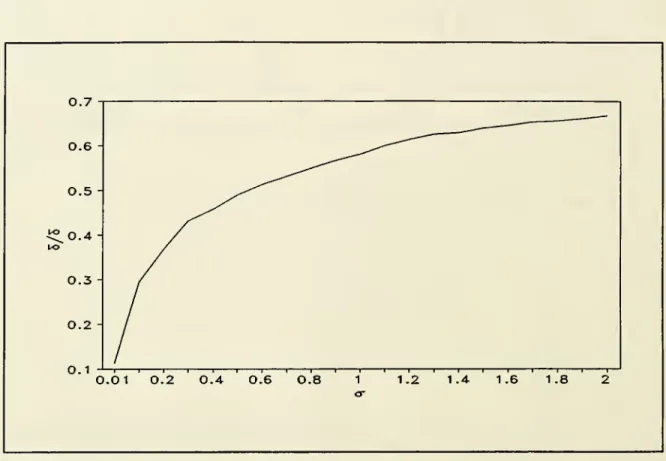
of the learning-by-doing effects (6,/8 )

9

. Fig.5

shows

different combinations of

5,/5

and

o

2_v

which

generate

p=0.9 and

q=0.76

when

aggregate shocks are normally distributed.

To

obtain the

same

persistence in

S

t, ahigher variance requires

more

increasingreturns.

The

reasonfor

this isthatthe greater the variance ofshocks, the

more

likely agents are toreceive a future

shock

less

than (Do-CD,. This lessens the expected future benefits

from

increasing returns

and

makes

agents both less likely to invest

and

less likely to

remain

investing

once

they

have done

so.

Thus

withincreasing returns of

22%

(8,/8=0.22) to

produce

the appropriate values of

p and q

we

require

a

2_v=0.05, but

when

G^O.Ol

we

need

only 8,/8

=ll%.

As

well asproviding persistence, intertemporal increasing returns generate considerable amplification ofthe productivity shock.

For

thecase

where

8,/8

=0.22

and

^=0.05,

even though

_cV

a

i

=

0.03, the variance of

AY

t is equal to 0.634. Relying only

on

a

Oq does not influence the values of cOq and go, and so (without loss ofgenerality) it is set to ensure the model

matches

mean

US

output growth.

single productivity

shock

to drive output fluctuations,

we

need

implausibly large learning-by-doing effects of

53%

to explain Hamilton's results.

But

with an additional additive disturbance in (1), as

assumed by Hamilton and

all econometric implementation of

unobserved

component

models, his results can be explained with very small

amounts

ofintertemporal increasing returns

and

aggregate

uncertainty.

Results

from

alternative studies confirm this finding that only small scale intertemporal increasing returns are necessary to generate empirically observed

regime

shift behavior.

Suzanne

Cooper

(1994) uses

monthly

industrial production

from

1931 to estimate a transition matrix similar

to (28).

To

match

her estimates of the transition probabilities (p=0.55

and

q=0.46) while also

matching

the variance of

US

GNP

growth

(again without resorting to

any

additional productivity disturbances other than a unique aggregate shock),

we

need

the saving in fixed costs arising

from

learning-by-doing to

be

only

around

3%

(i.e. 5[/5 =0.03).

Diebold

and

Rudebusch

(1994) estimate equations analogous to (28) using

US

industrial production (allowing for a time

dependent

T).

Assuming

only

one

disturbance

and

using theirestimated standard error for

AY,

to calibrate

o

_v2 (an

underestimate as this implicitly sets S,=l for all t),

we

find 8,/8

=0.8%

is sufficient to explain their results.

(ii)

The General Unobserved

Components

Model

Inthissubsection

we

use (15)

and

(16) toobtain estimatesof ourstructuralparameters.

These

equations represent a general statespace

model

and

requireassumptions regarding thedistribution of

idiosyncratic shocks before they can

be

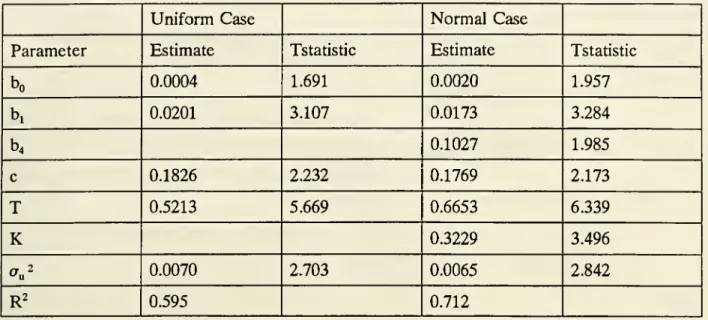
estimated.

We

examine

these equations

assuming

first that

idiosyncraticshocks are uniformly distributed

and

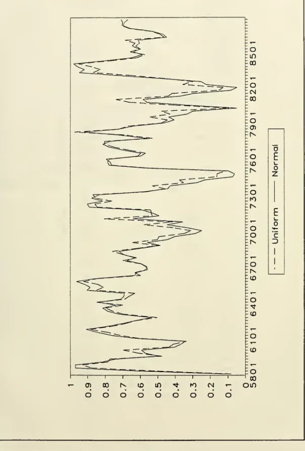
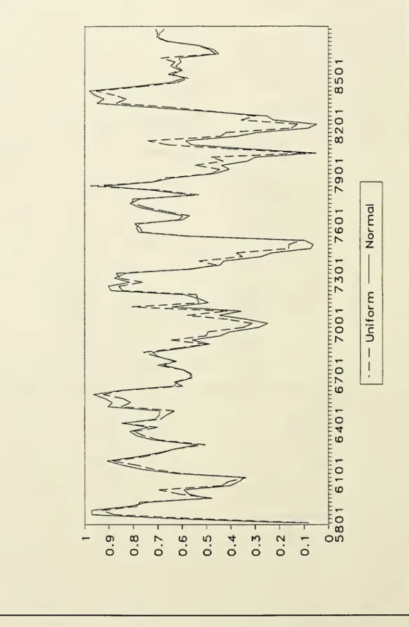
then thatthey are normallydistributed.

As

well as enablingus toassess therobustnessof ourestimatesofstructuralparameters theseassumptions allow

us to

examine

the importance of

asymmetries

in U.S. output fluctuations.

As

discussed above, the

assumption of

uniform

idiosyncratic shocks

removes any

asymmetry

inthestateequation.Estimating

(15)

and

(16) under different distributional assumptions therefore enables a simple heuristic test of

theimportance of asymmetries in U.S. business cycles.

Assuming

thatidiosyncratic shocks are uniformly distributed over therange [-a,a], (15)

and

(16) can

be

written as „ a-oin o>, v, (31) ' l

_2a

1 2a

M

2a

=c+ rs,_1+

u

t

where

thecoefficients _ty arefunctions ofthestructuralparameters u) ,co„ a, o^,

and

a,

and

aside

from

the squared disturbance in the

measurement

equation this is the standard return to normality

model

(e.g.

Harvey

(1989), ch.3). Various versions ofthis

model

have been

used to estimate the cyclical