Bayesian signal reconstruction, Markov random fields, and x-ray crystallography

To appear in Journal of the Optical Society of America A

Adaptive Bayesian Signal Reconstruction

with A Priori Model Implementation and

Synthetic Examples for X-ray

Crystallography

Peter C. Doerschuk

School of Electrical Engineering

Purdue University

West Lafayette, Indiana 47907-1285

(317) 494-1742

February 26, 1991

Abstract

In [1] a signal reconstruction problem motivated by X-ray crystallography is (ap-proximately) solved in a Bayesian statistical approach. The signal is zero-one, peri-odic, and substantial statistical a priori information is known, which is modeled with a Markov random field. The data are inaccurate magnitudes of the Fourier coefficients of the signal. The solution is explicit and the computational burden is independent of the signal dimension. In this paper a detailed parameterization of the a priori model appropriate for crystallography is proposed and symmetry-breaking parameters in the solution are used to perform data-dependent adaptation of the estimator. The

tation attempts to minimize the effects of the spherical model approximation used in the solution. Several examples in one and two dimensions based on simulated data are presented.

[1] Peter C. Doerschuk. Bayesian signal reconstruction, Markov random fields, and x-ray crystallography. Journal of the Optical Society of America A, 1991. To appear.

1

Introduction

In [1] a novel Bayesian statistical approach is presented to a class of phase-retrieval problems exemplified by the inverse problem of single-crystal X-ray crystallography. In this paper parameters are proposed in the a priori model that are suitable for modeling bond-length limitations in covalently-bound molecules, free parameters in the estimator are employed in order to design a data-dependent adaptive estimator, and several numerical examples in one and two dimensions based on simulated data are provided.

The situation from [1] is recalled in this and the following paragraph. There is a periodic object which takes only values zero and one, and the observer makes corrupted measurements, denoted Yk, of the magnitude of its Fourier transform. The goal is to reconstruct the object from these measurements and from a priori probabilistic information concerning the class of likely objects. One period of the object is modeled as a binary-valued finite-lattice MI\arkov random field (MRF) denoted

(,

and the corruption of the measurements is modeled as independent Gaussian random variables with k-dependent variances. Both the MRF and the Gaussian observation errors can be put in the form of energy functions with the corresponding probabilities in the form of the Gibbs distribution. A Bayesian conditional mean estimation problem is approximately solved. In order to compute E(Snl{y}) one computes averages. However, because only the magnitude of the Fourier transform is available, the definition of the coordinate system on the object is lost. For example, in one dimension, all information concerning the origin in the sense of translation and concerning the handedness in the sense of inversion through the origin (n -- -n) is lost. If one blindly averages over all configurations of {5}, the result is a DC field. Therefore, an additional term in the energy function is introduced which favors certain configurations. For example, in one dimension, the additional term breaks the symmetries of the previous energy function with respect to translation and

inversion. The term has the form of a convolution of the field O,. with a kernel function '?,.

The

n0,

are the free parameters alluded to above, and the subject of this paper is a method

for choosing them in a data-dependent fashion.

In solving the estimation problem in [1] two approximations were made. The first ap-proximation was the spherical model which relaxed the 0-1 nature of the lattice variables q,n. The second approximation was to evaluate integrals asymptotically as the observation noise variance approached zero. (Actually two different asymptotic problems were proposed and solved depending on whether the a priori energy function was scaled along with the observational energy function). Given these two approximations, explicit (e.g., no numeri-cal quadratures or nonlinear optimizations) formulae were computed for an approximation, denoted m,, to E(,lj{y}) as a function of

4'

and y. These formulae are easy to comnpute, can accommodate missing data and varying observation noise variance, and are essentially

the same in any dimensional space.

For any choice of P, this is a valid Bayesian estimation problem. Therefore, the goal is to choose 4, in an intelligent fashion. One natural approach, which is the approach taken here, is to try to choose 4, or equivalently, the estimation problem, to minimize the effects of the two approximations made in the solution of the estimation problem.

In this paragraph the Hamiltonian is recalled from [1]. The Hamiltonian is in three parts-the a priori probability part Hapriori, parts-the conditional observational probability part Hobs, and the symmetry breaking part Hs'.b. That is,

H = Hapriori + Hobs + Hs.b.

Equations are stated for the one-dimensional case. In d dimensions exactly the same equa-tions hold with indices, lattice dimensions, and sums all expanded to d dimensions. The a priori part is the most general shift-invariant quadratic, specifically,

L-1 L-1 Un =

S

E: 0.+l 1w2(n1, n2) ln+n2 +w n (1 ) nl =0 Ln2=0 L-1 Hapriori = E U n=O

lattice spacings. The conditional observational part is Gaussian, specifically, Zk = ID k12 L-1 4)= Oen-jnk2L L-i 1 Hobs 2(-Hs k= 2 2 (Yk - Zk(f0})) X

where Yk and ak are observed in the experiment. However, the ark values are assumed to

be exact. Finally, the symmetry breaking part is a convolution with the kernel function b, specifically,

L-1

H.b.

= qL

n=O .,

where On is real and periodic with period L.

In this paragraph the asymptotics are recalled from [1]. Two different asymptotic limits are considered. The first limit, denoted Problem 1, is purely a small observation noise limit. That is, the observation noise variance a2 satisfies a = &2 and A T oo. The second limit, denoted Problem 2, combines the small observation noise limit with a proportional scaling of the a priori Hamiltonian. That is, the observation noise variance a2 and the parameters W2(k1, k2) and w1 from the a priori portion of the Hamiltonian satisfy ak = ;lc

W2(kl, k2) = AXW 2(ki, k2), W1 = AXWi, A T oo, and X is a fixed real number.

The remainder of this paper is organized in the following fashion. In Section 2 a parame-terization of the a priori Hamiltonian is described that is appropriate for X-ray crystallogra-phy. In Section 3 an optimization problem is described for the choice of b. Implementation issues are briefly discussed in Section 4. In Section 5 one-dimensional examples are pre-sented which emphasize the need to break the symmetries discussed above. In Section 6 a one-dimensional example is presented which is sufficiently small such that it is possible to compute estimator performance statistics versus observation noise intensity for the exact conditional mean estimator, the approximations to the conditional mean estimator ( with either definition of the asymptotics), and the trivial estimator that simply takes a random

sample from the a priori distribution for its estimate. A two-dimensional example is pre-sented in Section 7. Finally, in Section 8 the results to date are discussed and directions for future research are described.

2

Use

of Hapriori

in X-Ray Crystallography

In this section one method for using the quadratic a priori Hamiltonian Hapri°_{ri to model}

bond-length limitations in covalently bound molecules is described. By interpreting I I as absolute value in one dimension or as Euclidean norm in higher dimensions, the following applies for arbitrary dimension of the signal.

Define a minimum (maximum) bond length 11 (12) measured in lattice spacings. Assume that there is an atom at site no. Therefore, qn,, = 1. In order to avoid the presence of a neighboring atom at less than the minimum bond length, the a priori probability function is low if there is an atom in the region {nlln - nol < II}. In addition, in order to avoid unbound atoms, the a priori probability function is low if there is no neighboring atom in the region {nlll < In - nol < 12}. In order to use these ideas with the quadratic Ha p"'i°'

defined previously, the penalty on crowding (i.e., an atom in the region {nn - noI < 1

}))

must become progressively greater as more atoms fall in the region and the penalty on being unbound (i.e., {nlll < In - nol < 12}) must become progressively smaller as more atoms fall in the region. (Note, however, that as more atoms are present in this region they in turn will become crowded with respect to each other, thereby lowering the a priori probability function again). The penalties described here are associated with site no and therefore w1,

w2 should be chosen so that the penalties appear in u,0 (eqn. 1). Since there are no penalties

that depend only on the value of a single site, wl = 0. Since the penalties only occur when q~o = 1, it would be convenient to choose w2(nl,n 2) so that it is zero unless nl = 0. Since

w2(ni,n2) = ½(C2(nl,n2)+ Wt2(n2,nj)) where dt2(nl, n2) is defined by

w2(nl, n2) = O n1# O, Vn2

P1 if 1 < In21 < 11

tb2(0, n2) = P2 if 11 < In2I< 12

0O otherwise

and where pl > 0, P2 < 0, and 1 < 11 < 12. Generalizations to Hamiltonians that include a quadratic penalty on deviations from a desired valence number are also straightforward.

To this point in the present paper and throughout [1], this model and estimator have been motivated from the perspective of atomic resolution X-ray crystallography where the lattice variables are the presence or absence of an atom at that location. However, there are low resolution structures of large molecules (e.g., proteins) that might also be addressed. In the low resolution protein setting, one is interested in locating the path in three dimensions of a solid "tube" of high electron density that follows the polypeptide backbone in a background of relatively low electron density. The new interpretation of the lattice variables would then be that 0 corresponds to background and 1 corresponds to polypeptide backbone, which is approximated to have only one value of electron density. The purpose of the a priori Hamiltonian HaPriori would then be quite different. Specifically, it would seek to make the occupied sites (the l's) form a connected solid tube rather than scattering through space. Therefore, it would more resemble a ferromagnetic Ising model Hamiltonian than the bond-length Hamiltonian described in the previous paragraphs. After this change in interpretation of the lattice variables and change in the constants in the a priori Hamiltonian, the remainder of the calculation in [1] would be unaltered.

3

The Choice of

4

The symmetry breaking portion of the Hamiltonian, HS b', contains the parameters On, and for any choice of ;bn an approximation to the Bayesian conditional mean estimator was computed in [1]. These degrees of freedom are used to design an adaptive estimator.

As described in the Introduction, the calculations of [1] contain two approximations, namely the spherical and asymptotic approximations. The asymptotic approximation is of less concern because it can be improved on by taking additional terms in the asymptotic series and because the crystallography problem is in fact a small-noise problem. However, the spherical approximation, by relaxing the atomicity of the electron density which has been central to successful direct methods in crystallography, is of more concern. In addi-tion, natural improvements on the spherical approximation are difficult to compute because they couple the Fourier coefficients. Therefore, the adaptive estimation scheme focuses on decreasing the effects of the spherical approximation.

The idea is to choose a new Vb for each data set such that the choice minimizes a cost function C. C is a function both of ibn and of the unthresholded approximations mn to

the conditional expectations E(Ol{y}) that result from using ibn in the estimator. The

cost function is a linear combination C = -ylCl + 72C2 + 73C3 of three individual costs. C1 attempts to improve on the spherical model by penalizing a manifestation of the spherical model's relaxation of the 0-1 constraints on the lattice variables. C₂ attempts to control the energy in ,bn so that it neither vanishes and thereby fails to break the symmetries nor dominates the Hamiltonian. C3 attempts to select an estimator that is confident of its

answer, that is, an estimator where m, are near 0 or 1.

For binary lattice variables the conditional expectations are constrained to [0,

1].

The es-timates computed using the spherical approximation routinely violate this condition. There-fore, if m, is the computed approximation to E(qSnl{y}), ?1 is chosen to minimize a cost

function that penalizes mn, i [0, 1]. The work described here uses the simple cost function

C1 = Z E i(mn)

(x-_1)2 if x>1

c,(x) = 0 if 0 < x f < 1

x2 if x < 0

or to grow too large and dominate the estimator. Therefore, deviations in energy from a desired energy Eo are penalized with the cost function

C= (114'11 - Eo) 2

where

Ilxll,

= (E xP)l/P. Choice of Eo is discussed in the following section.

Finally, among all the estimators parameterized by

4,

it is desirable to choose a confident estimator, that is, an estimator for which the resulting m, are near 0 and 1. Therefore deviations in mn from 0 and 1 are penalized by using the cost function

c3

= E O3(mn)

(0 if x> 1X uf3(X) = (X- 1)2x2 if 0 < X <

0 if x<0

(I prefer to penalize mn > 1 and mn < 0 through C1 only).

The costs C1 and C3 depend on mn, the approximation to the expectation E(,,Il{y}),

which in turn is a function of

4'.

When optimizing

4

the m, are recomputed for each new

value of

4.

There are obviously many other ways in which one might set

4'.

One natural entirely different category of methods would be to set

4'

so that the resulting Bayesian estimator has some desirable statistical property. Here the choice would be made once forever according to some ensemble criteria while in the method described above the choice is made for each data set according to a pathwise criteria. For any

4,

the Bayesian conditional mean estimator minimizes the conditional expectation of the squared difference between the actual and estimated fields. One might then choose

4

to minimize higher order statistics or a special discrete class of errors that are particularly important from the application perspective.

4

Implementation of the Vb Optimization

When computing

4',

globally optimal solutions were not sought. Rather I have thought in terms of downhill search starting from an initial condition pi.'C where the initial condition (1) has a clear symmetry-breaking interpretation and (2) is used to set E0 in C2 by Eo = I[l,i'.c.I 2

This choice seems preferable because it is computationally straightforward and because it attempts to keep some balance between the symmetry-breaking role of

4,

only implicitly included in the optimization criteria, and the optimization role of

4'

(since a simple downhill optimization will presumably remain in some domain of attraction of the initial condition and the initial condition has a clear symmetry-breaking interpretation).

0

O

if

s

=

O

For one-dimensional problems the initial condition was , . ( 0

n (L - n)/L iif 72 0 0 This choice sets Hs''b _{to be the first moment of the field O, and therefore clearly breaks}

translational symmetry. Two-dimensional problems have more types of symmetries than one-dimensional problems and an initial condition that clearly breaks more than transla-tional symmetry is desirable. In the work described here the initial condition was '/C' = 0'(n1 ; L1, al)V)(n2; L2, a2) where L1 and L2 are the dimensions of the lattice, a1 and a2 are

constants, and

fO if n= 0

4(n;L,a) = . ( ( 2)

( (L-n)(l + a(L-n))/L if n 0

(

This choice breaks translational and inversion (equivalently, rotations by Ir) symmetries. If L1 = L2 then rotations by n' are also symmetry operators and these symmetries are also

broken by this choice of ?P.

Though the initial condition for

4

in two-dimensional problems is a product of functions of individual coordinates, the optimization considered any two-dimensional ;, not restricted to this product form. However, it may be sufficient and would certainly save computational expense to consider throughout the optimization only

4

with the product form.

A very inefficient scheme was used for optimizing

4

which, however, results in an un-constrained optimization problem. The inefficiency stems from the parameterization. Recall

from [1] that the estimator has the following structure. First, fix

4'.

Second, compute ap-proximations M/lk to E(Dkl{y}), the conditional expectations of the Fourier coefficients of the field q,. The formulae for this computation are in terms of Sk, the Fourier coefficients

of

',n

and the data {y}. Third, compute approximations m, to E(Sql{y}), the conditional expectation of the field, by computing the inverse Fourier series of Mk. Fourth, threshold the rn2 to compute the estimated field.

The L real variables bn n E {O,..., L - 1} were used to parameterize

4b.

Because each of these variables independently ranges over all of R, methods for unconstrained optimization problems can be applied. However, a computational penalty is paid because first 0n must be transformed into 'Tk, at the cost of one Fourier series, and then Mk must be transformed into m,, at the cost of a second Fourier series. If the parameterization was T0 E R, z T k, and

Ij'kl (k E {1,... , L2 }), then the optimization is no longer unconstrained since ZL k E [0, 27r)

and lIkl E [0, ~o), but the cost of one of the Fourier series calculations is avoided. Note in this regard that C2can easily be computed in terms of 4,,. or in terms of IXkl. Also note that

the above is purely a discussion of efficiency per iteration. The behavior of the optimization criteria as a function of the parameterization (e.g., straight versus highly curved valleys) will determine the number of iterations required and this aspect has not been considered at all.

Furthermore, an inefficient multidimensional downhill simplex method [2] was used to solve the unconstrained optimization problem. This method uses function evaluations but no derivatives and attempts to move a nondegenerate simplex in RL defined originally by L + 1 initial condition vectors downhill by simple geometric moves (e.g., reflection of the vertex with the highest function value through the opposite face of the simplex to a position with a lower function value) until the simplex arrives at a minimum. This algorithm was chosen because the software is robust and was easily available. As mentioned in the previous section, at each step mn (the approximation to E(,nlI{y})) is recomputed for each choice of

Finally, all the equations, both for the one- and two-dimensional cases, are for odd

11--~~"

dimensioned lattices. As mentioned in [1], this case was considered because the fact that q, is real constrains ek, its Fourier coefficients. Specifically, in one dimension, it implies

that "k = D*-k. For L even there are therefore two coefficients that are guaranteed real (more in higher dimensions) while for L odd there is one such coefficient in any dimension. Therefore the equations are much simpler for L odd. However, L odd is unfavorable from the computational point of view because it is incompatible with using power of two Fast Fourier Transforms. In one dimension the Fourier series was computed by explicit summation at a cost proportional to L2 while in two dimensions the Fourier series was computed by a one-dimensional chirp z transform on rows and then on columns. In light. of the inefficient parameterization, software, and Fourier series situation, measures of algorithm speed are not reported.

In [1] a very brief sketch was given of an algorithm for locating the critical point in

the asymptotics that is exact, noniterative, and requires only order L computation. This algorithm is described more fully in the Appendix. In the examples described in this paper, there is always a single critical point so the simple formulae of [1] apply. In fact, in the problems where I have investigated, there is only a single maximum for the exponent which determines the critical point.

5

One-Dimensional Examples

These examples are included to emphasize the importance of the symmetry breaking role of

The calculations of this section use the Problem 2 asymptotics where the observational Hamiltonian Ho° b and a priori Hamiltonian Hapri°ri are both scaled by the asymptotic pa-rameter and the ratio between their scalings is X. In the Hamiltonian of Sections 1 and 2 take

or = =o 2 = 0.1 Vk E {0 ... , L-1}, X = 1, q 1, , P = p2 p11 = -2, = 4, 12 = 6, and L = 27. For the adaptive estimator design cost take either CO = C1 + C2 or C' = Cl + C2 + C3. Two

simulations are described based on two different choices of the underlying field {q}. InI both cases the simulated data are pseudo Gaussian random numbers with variance 0' 2 added to

the Fourier coefficients of the field. Since the fields have either two or three occupied sites, these noise levels correspond well to the 1 to 3 percent errors in real crystallographic data [3, p. 193].

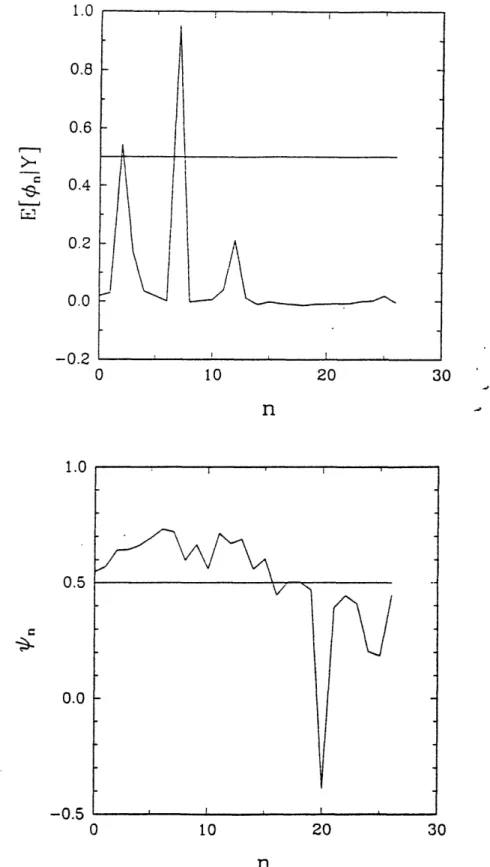
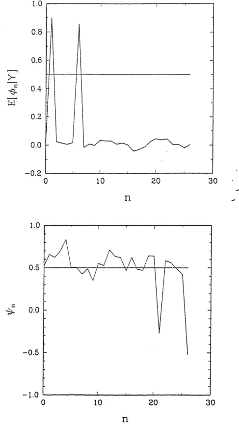
f

0 if

nh{1,5}

For simulated data based on the field 2 if n using cost C'

(respec-1 if

nE{1,5}

tively, Cl) the approximate conditional expectations are shown in Figure la (respectively, Figure 2a) and optimized byn functions are shown in Figure lb (respectively, Figure 2b). In both cases the thresholded estimate will be exactly correct though in the case of CO (i.e., not specifically selecting a confident estimator), the estimator almost fails to locate the first occupied site.

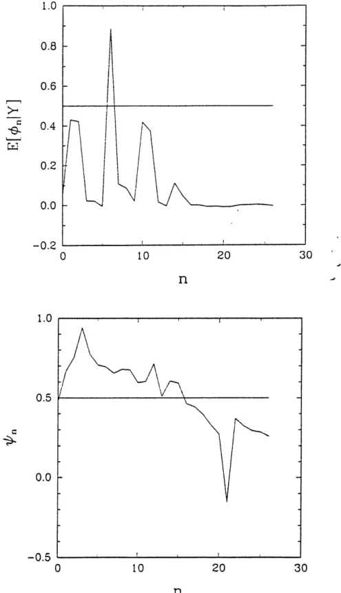
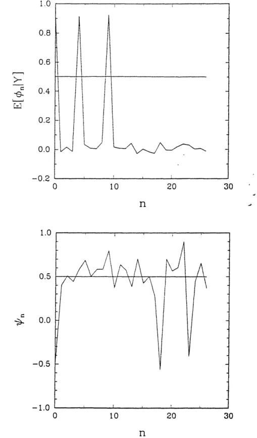
For simulated data based on the field 3 = f n 1, 5, 9 using cost CO (respec-.1 if n E {1,5,9}

tively, Cl) the approximate conditional expectations are shown in Figure 3a (respectively, Figure 4a) and optimized ,n functions are shown in Figure 3b (respectively, Figure 4b). In the case of CO _{(i.e., not specifically selecting a confident estimator), the estimator fails to}

locate the first and third occupied sites. Instead there are two broad low peaks. The reason for the broad low peaks is a failure to adequately break inversion symmetry. Specifically, the left (respectively, right) half of the left peak, the central peak, and the left (respectively, right) half of the right peak corresponds to intervals of 5 and 4 (respectively, 4 and 5) corre-sponding to the signal and the inverted signal. When C' is used, this inversion symmetry is broken and only one of the signal and its inversion (specifically its inversion) are substantially represented in the a posteriori expectation and the thresholded estimate is exactly correct.

6

Estimator Performance Statistics Versus

Observa-tion Noise Intensity

This section describes results concerning the estimator performance statistics versus obser-vation noise intensity for the exact conditional mean estimator, the two approximations to the conditional mean estimator (that is, the two definitions of the asymptotics), and the trivial estimator that disregards the data and simply takes a random sample from the a pri-ori distribution for its estimate. Comparison of the performance of the nontrivial and trivial estimators for different performance measures provides measures of the signal to noise ratio improvement due to the use of the nontrivial estimator. To perform these- calculations the lattice must be very small-one-dimensional with L = 17 sites-because the computation is done by Monte Carlo methods and the calculation of an individual estimate for the exact estimator is done by exhaustive enumeration.

The data is generated by first computing configurations of the Hapriori described in Sec-tion 2 and then computing the observaSec-tional transformaSec-tion (Fourier transform followed by magnitude squared) and adding Gaussian pseudo-random variables. The combination of configuration generation, observational transformation, and additive noise is denoted the "forward" problem.

The three nontrivial inverse problems are matched to the forward problem, that is, they share the same values for the parameters, except that the configurations in the forward problem are chosen with q = 0 for the symmetry breaking parameter.

Hapriori has parameters w1 = 0, 11 = 3, 12 = 5, Pi = 1.5, and p2 = -0.5. The observational

transformation has no parameters. The additive white pseudo-random Gaussian noise is parameterized by its standard deviation, denoted ok, which is constant over k. A range of values for cr were considered. See the figures. In all calculations, there are no missing observations.

addition of q = 1.0.

The approximate conditional mean inverse problems use -yl = 7Y2 = y3 = 1 in the opti-mization criteria for the design of

4'.

Two parameter sets are considered which differ ill the role of A which results in a difference in only the values for A, X, and a. Both are parameter sets such that the forward and inverse problems are matched except for q. The first set of parameters is matched to the forward problem with the exception of q = 1.0 (as in the exact inverse problem) and has in addition X = 1.0, A = 1.0, and d = 1.0. The second set

of parameters uses A instead of a'2 _{to control the accuracy of the observations. Then}

x

_is

used to compensate in Hapriori for the value of A :A 1. Specifically, the quantities A and X,\

have the same value in both parameter sets but in the first set A = 1 while in the second set ac = 1. For Problem 2 asymptotics both the first and second set of parameters are used. As expected, both calculations yield the same results. This fact amounts to a numerical check on the equations' and software. For Problem 1 asymptotics only the first set of parameters are used.

Statistics are collected on N = 1000 trials for each value of a. The underlying fields {X}

are drawn from the probability mass function 7 exp(,-Hapriori) where Z _=

Z{¢

exp(-3HaPior-)

using the Metropolis algorithm2. At a given a, the same set of stochastic realizations of the forward problem is used for all three nontrivial estimators. Since 1000 m 210 and there are only 217 configurations of the underlying lattice random variables, the lattice variable con-tribution to the total randomness in the measurements is fairly well sampled. (There are actually fewer distinguishable configurations because translations and inversions are unob-servable).

Two measures of performance are considered. Both measures are expectations which are 1_{To see that the equations are invariant under parameter changes such that ~ and XA are constant, it is}

helpful to introduce a new Lagrange variable r' to replace r (see [1, Section 10]) where r' = rA.

2_{The initial condition for the Metropolis algorithm is independent pseudo random binary numbers alt}

each site with equal probability of 0 and 1, the system is equilibrated for 200000 trials, and then the result of every 1 0 0 0 0th trial is used.

approximately computed by averaging the results of the N trials3_{. Let On be an estimate of}

0b,. Because the phase of q5n is not measured, ~n+no (translation by no) or _-n (inversion

through the origin) are equally satisfactory estimates. Therefore in this section min means a minimization over a possible inversion through the origin and a translation applied to

On. Let IIxllp = (En IlxnP)"/P. The first measure is the expected value of the 12 norm of the difference between the true and reconstructed signals after a possible translation and

reflection in order to achieve the best match,4 _{i.e., E(1}

2) = Emin Il -

$112.

Let tL(o, )

be the minimum number of lattice sites where n, =7 ,n and the minimum is taken over

a possible inversion through the origin and a translation of s. Note that min j - ~112 =

min I - 11, = /( , ). Therefore the performance results for mean squared error, mean absolute error, and mean number of lattice site differences are all the same. The variability of performance around the average performance is also important. Therefore, for average performance measured in the sense of E(12), the variability of performance in the sense of

the standard deviation SD(12) is also computed, i.e., SD(12) = Varmin I1l-

q11

2

-The second measure, denoted fperfect, is the probability of an error-free estimate, i.e.,

On = On for all n, again modulo inversion and translation. That is, fperfect _{= Pr(P(O, () =} 1 if i=j

0) = E6S,(0,),0 where Si,j =

0 ifi j

Statistics on the trivial estimator are computed in the following fashion. For the previous computations, 13 sets of 1000 random samples from the a priori distribution (q = 0) were computed. For this computation take all unordered pairs of not equal sets (78 total), label one as truth and one as estimate (the labeling does not matter since the cost functions are invariant under exchange of truth and estimate), compute performance statistics for that pair, and finally average the performance statistics over all pairs considered. The results are

3

Weighting by the probability mass function is not necessary since the configurations are drawn from the probability mass function.

4

Recall from [1] that the conditional mean estimator is optimal for the cost function II - j112. That is, among all estimators k({y}), the conditional mean estimator is the estimator that minimizes E(Ik -oll {'y} ).

nperfect = 74.3077, E(12) = 1.4792, and SD(12) = 0.5346.

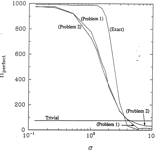
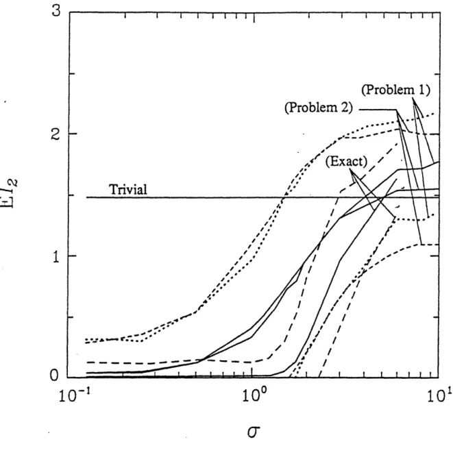
Figures 5 and 6 show plots of nperfect = fperfectN (Figure 5) and E(12) (Figure 6) versus

a. On both plots the three a-dependent traces plotted with solid lines show performance for the exact conditional mean estimator (the best performance), the Problem 2 asymptotics approximate estimator, and the Problem 1 asymptotics approximate estimator while the or-independent trace shows performance for the trivial estimator that disregards the data. The traces for the approximate estimators only differ significantly at high a where the Problem 2 estimator consistently outperforms the Problem 1 estimator. On Figure 6 the traces plotted with dotted lines show plus/minus one sample standard deviation (i.e.,. SD(1₂)) relative to E(12) for the three nontrivial estimators. The reason that the plots uo not have the

two highest a data points for the exact computation is that the number of probabilistically important configurations increases as a increases. The running time of the current algorithm for the exact computation is sensitive to this number and becomes prohibitively long.

The maximal signal possible at any k in this problem is L = 17. Therefore, ignoring the constraints placed on the lattice configuration by the a priori distribution, the large r region reaches into the realm of rather noisy data. This is born out by the fact that the exact and trivial (observation independent) estimators provide rather similar performance by a = 6. Similarly, the small or region represents rather clean data. The general character of the performance is that at low and high o- all three nontrivial estimators provide rather similar performance while in the transition zone the exact estimator provides good performance to slightly higher a than the approximate estimators. These general characteristics are common in exact versus approximate nonlinear filters, e.g., in phase-locked loops [4, Chapter 6]. Note that at high oa with respect to the nperfect performance measure the exact estimator performs less well than the approximate estimators, reflecting the fact that the exact conditional mean

estimator is not optimal for the nperfect performance criteria.

The fact that the Problem 2 estimator outperforms the Problem 1 estimator at high cr is expected. Recall that the Problem 2 estimator weights the a priori Hamiltonian Hap

'i °ri by

the asymptotic parameter A while the Problem 1 estimator does not. Since the estimators are computed in the A -- oo limit (even though they are used at finite A), the Problem 2 formulation relies more on a priori information and at high a a priori information is the only available information.

In Figure 6 the mean plus/minus one standard deviation lines are quite distant from the mean. One of the reasons for this is the discrete nature of the ~ estimates. Since min | -+2 = #(~,

¢)

and it takes on only small integer values, the standard deviation of

min II -+112 is larger than might be expected because all deviations from mean performance

must be at least a certain minimal distance away. In the Table a complete set of histograms as a- varies are shown for the number of trials (out of N total trials) in which [t(6, 6) takes each of its observed values when ~ is computed by the exact conditional mean estimator.

At high a, all three nontrivial estimators give estimates with higher values of E(12)

than the trivial estimator that disregards the data. I attribute this to the q = 1 used to break the symmetries in the nontrivial estimators, which is not equal to the actual value of q = 0 used both to select the true configurations from the a priori distribution and to select the estimated configurations in the trivial estimator. One could compute a second trivial estimator which again disregards the data but draws from a distribution with q = 1. I did not do this because this estimate is (slightly) more costly to compute than the q = 0 estimate and will have poorer performance so there is no logical reason to use such an estimator. In addition there may be a statistical effect since the trivial estimator's performance is based on a far larger number of trials.

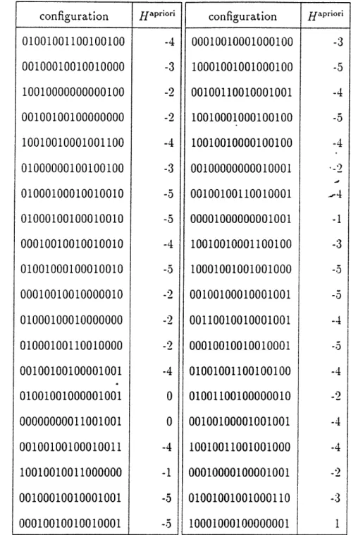
In Figure 7 a small subset of the truth configurations used in these simulations are shown. While the small size and the one-dimensional nature of the lattice preclude a really "molecular" appearance, still the basic idea is present-the l's, which correspond to the atoms, are generally neither adjacent nor isolated in both directions by great distances. Rather, the l's occur on average one "covalent bond length" from each other. Note that the boundary conditions for this space group are the standard toroidal boundary conditions so that 1's

near an end may be bound to l's near the other end.

7

A Two-Dimensional Example

In one-dimensional examples there is no concept of bond angle and therefore there are surprisingly few degrees of freedom in a configuration that has a low value for Hapri° ri. In this section a two dimensional example is presented which demonstrates that the approximate estimators can work in situations with these additional degrees of freedom which are only indirectly constrained by the bond-length oriented a priori Hamiltonian. Also, this example. though still small, has many more lattice sites than any of the previous examples.

The lattice measures 9 by 13 sites. The true configuration has 7 occupied sites located at positions (5,10), (2,8), (3,5), (5,3), (4,0), (1,0), and (0,3). The observation noise has

variance 0.75 constant over k. The Hapri°ri of Section 2 has parameters pi = 1.0, P2 = -2.0,

11 = 2.3, and 12 = 4.2. The approximate conditional mean inverse problem uses Problem 2

asymptotics and has parameters q = 1, X = 1, A = 1, and P = 1. The initial condition for the b optimization has parameters al = = 0.111111 and cr2 = 1 = 0.0769231. This

choice of ac and a2 balances the linear and quadratic terms in the ib initial condition in the sense that the linear term (L - n) and the quadratic term ac(L - n)2 _{evaluated at n = 0 (see}

eqn. 2) have the same value in both coordinate directions.

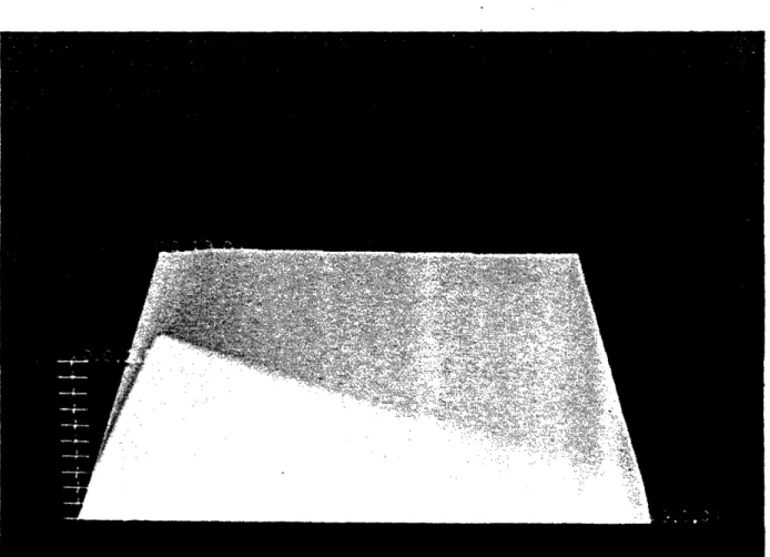
Results for the approximate conditional mean estimator are shown in Figures 8-11. Fig-ure 8 shows the initial condition for Ob as a smooth surface in three dimensions above the two-dimensional lattice array. Figure 9 shows the optimized V in the same format as Figure S. Note, as expected in light of the simple optimization scheme, that the initial and terminal

b are qualitatively quite similar. Therefore the optimization, which does not explicitly in-clude a measure of symmetry-breaking performance, has probably not greatly altered the symmetry breaking built into the initial condition ¢. Figure 10 shows the true b field and the estimated 4b field. Since these are binary fields, they are shown as patterns of occupied

sites rather than as projections of surfaces. The estimate is exactly correct, though shifted from the true configuration by an inversion through the origin followed by a translation by the vector (5,11). Better performance cannot be hoped for since inversion and translation do not effect the magnitude of the Fourier transform coefficients. Finally, Figure 11 shows the final (i.e., computed with the optimized b) approximation to E(Obl{y}), the conditional expectation of the lattice field, in the same format as Figures 8 and 9. Figure 10, the es-timated b field, results from thresholding Figure 11 at value l. In light of the large local maxima, it is straightforward to anticipate the result of the thresholding operation.

8

Discussion and Future Directions

In this paper a parameterization of Hapriori that is appropriate for crystallography is proposed; data-adaptive ideas for the choice of $, the convolutional kernel in the symmetry-breaking

Hs.b., are described; and several numerical examples in one and two dimensions on

simu-lated data are given. The examples included a tiny one-dimensional problem where it is computationally practical to compute the estimator performance statistics versus observa-tion noise intensity for the exact condiobserva-tional mean estimator by brute force and compare with the approximate estimators. These examples, though small in size, demonstrate that these approximations based on the spherical model and small-noise asymptotics provide rea-sonable performance relative to the exact conditional mean estimator, which is extremlely expensive to compute. In the future superior optimization schemes are needed, as discussed in Section 4, in order to allow larger problems to be considered and more general space group symmetries need to be included here and in [1].

9

Acknowledgements

The use of ideas from statistical mechanics (e.g., the spherical model) and Markov ran-dom fields grew out of discussions with Professor Sanjoy K. Mitter while the author was a Postdoctoral Associate at the Laboratory for Information and Decision Systems at M.I.T., Cambridge, MA. I would like to thank Professors Sanjoy K. Mitter and Alan S. Willsky for technical interest and financial support and Paul Friedman for the initial versions of the software for the MRF simulator and the exact conditional mean estimator used in Section 6. A detailed reading by Professor Willsky greatly improved the manuscript. This work was supported at M.I.T. by the Air Force Office of Scientific Research (AFOSR-89-0276), the Army Research Office (DAAL03-86-K-0171), and the National Science Foundation (ECS-8700903) and at Purdue University by a Whirlpool Faculty Fellowship and the School of Electrical Engineering, Purdue University.

10

Appendix

This appendix is based on the results of [1, Section 10] and uses the definitions of that paper. In this appendix an algorithm is described which efficiently solves for the critical point, that is the constrained global minimum, of OHx. The location of the critical point is needed in order to compute the small-noise asymptotic evaluation of the integrals required for the conditional-mean Bayesian estimator. In the process of computing the global minimum, all local minimum are also located.

In the case r = Lb ,2b for some k E {1,.. , L-l - B I simply set pk = 0 while in theory Pk is undetermined (though nonnegative) and I should eventually integrate over a manifold when computing the asymptotics of the integrals. The manifold will not be all of pi. > 0 because if Ptk is too large, then the constraint equation will not have a real root for po.

There are three straightforward initialization steps followed by a loop over at most ±L + 1

elements

Initialization (1). Define

L L-1

Ck = (bk,2a + bk,2b) k E {1,.. , 2 }

Initialization (2). Define kj E {I1,... L} j E {1,..., L-} a permutation of {1,. L-} such that Ck, < Ck2 < ... < CkL_. Define jmax = max{jlkj E {1,. . . - B}, that is,

Ckjmax is the largest c for which no observation was taken among frequencies k y 0. If {jiki

E

{1,... L } _ B} = 0, then set jmax = 0.

Initialization (3). Define Ij C R j C {1,... L-1 + 1} by

(-oo, Ckl) if j = 1

I= [ck_, ,ck,) ifj E {2,... L, }

[CkL_,,l) ifj = -2+

Loop (1). Fix j* E {jmax + 1,., L,. + 1}. The algorithm will eventually consider every element of this set.

Loop (2). Assume r e Ij..

Loop (3). By Loop (2), if kj E B then

3(T =b

k2b)k

4 J if j > j'

0 iifj < j

while if kj E {1,..., }-B then

Pk, = 0.

Note that these are not yet computable because r is not yet known.

Loop (4). Use the constraint condition and the gradient condition at k = 0 to solve for Po and r. Specifically, define

2 bk,,2a

+

bk,,2b do(j*,B) = -bka

(f

... L_-1 }-Bo 2 1 di(j*, B) =- bk2 j3{j. L }-B k,,4a -99

where if j* + 1 then

{j*,

.. L} = 0 and the sums are zero. Both sums are

2 2

computable at this point. The constraint condition is

Po - po + do(j*,B) - rd(j*, B) = 0 and the k = 0 component of the gradient condition is

-bo,lb- 2(bo,2a + bo,2b)po + 4bo,4aP3 + r(LPo 1) = 0 (4)

Assume dl(j*, B) = 0. Then eqn. 3 simplifies to 1 2

Po - po do(j*,B) = 0

which determines the po roots and there are exactly two possibly equal choices. If the roots are complex conjugates then there are no feasible solutions. For each real root, if the root is

L, then r for that root is undetermined. Otherwise eqn. 4 specifies that

-bo,lb - 2(b, 2a + bo,2b)po + 4bo,4ap3

1 2

T Po

Assume dl(j*, B) : 0. Then eqn. 3 can be solved for r giving ,. =

L Po do+ o(j' B) di(j*, B) Use of this result in eqn. 4 gives

P3

2

+ 4b 4dl(j B) + p

(2 )

+po -2(bo,2a + bo,2b)dl(j*, B) + ~do(j*, B) + 1

+ (-bo,lbdl(j*, B) - do(j*, B)) = 0

which determines the po roots and there are exactly three possibly equal choices. One choice is sure to be real while a pair may be complex conjugates and thus not acceptable. Then, for each real root, eqn. 5 specifies the corresponding r.

If Po ¢ R or 7 ¢ Ij. then discard that solution. For each retained solution p0 T. use the

equations of Loop (3) to compute pk k E {1,...-, } and then compute 3H,\. 23

Loop (5). Among the values of HxA found in Step (7) (there may be none) and the

minimum value of /Hx found so far from other j*, save the minimum value and the -, po, Pk Ik E {1,..., L1 } for which the value occurred.

Loop (6). If all j* e {jmax + 1, ... L + 1 have been considered then the result from

the most recent iteration of Loop (5) is optimal and the algorithm terminates. Otherwise, return to Loop (1) and select a new value for j'.

References

[1] Peter C. Doerschuk. Bayesian signal reconstruction, Markov random fields, and x-ray crystallography. Journal of the Optical Society of America A, 1991. To appear.

[2] William H. Press, Brian P. Flannery, Saul A. Teukolsky, and William T. Vetterling. Numerical Recipes in C: The Art of Scientific Computing. Cambridge University Press. Cambridge, 1988.

[3] George H. Stout and Lyle H. Jensen. X-ray Structure Determination: A Practical Guide. Macmillan Publishing Co., Inc., New York, 1968.

[4] Andrew J. Viterbi. Principles of Coherent Communication. McGraw-Hill Book Compally New York, 1966.

1.0 0.8 0.6 >-I 0.4 0.2 0.0 -0.2 0 10 20 30

n

1.0 0.5 0.0 -0.5 0 tO 20 30

n

Figure 1: Results for Two Occupied Sites Using Cost C°_{. Part a: Conditional Expectations}

Before Thresholding. Part b: Optimized n-.

1.0 0.8 0.6 S 0.4 0.2 0.0 -0.2 0 10 20 30 n 1.0 0.5 0.0 -0.5 -1'0 . . I . [ ! 0 10 20 30 n

Figure 2: Results for Two Occupied Sites Using Cost C'. Part a: Conditional Expectations Before Thresholding. Part b: Optimized ?L,.

1.0 0.8 0.6 .S. 0.4 0.2 0.0 -0.2 0 10 20 30 n 1.0 0.5 0.0 -0.5 0 10 20 30

n

Figure 3: Results for Three Occupied Sites Using Cost CO. Part a: Conditional Expectations Before Thresholding. Part b: Optimized i,,.

1.0 0.8 0.6 C 0.4 0.2 0.0 -0.2 0 10 20 30 n 1.0 0.5 0.0 -0.5

-1.0

0 10 20 30

n

Figure 4: Results for Three Occupied Sites Using Cost C1. Part a: Conditional Expectatioins Before Thresholding. Part b: Optimized 0,.

1000

i i

I I i

(Problem 1)

800

(Problem 2)

(Exact)

600

400

200

(Problem 2)

Trivial

(Problem 1)

10-

₁₀

_-

₁₀

°

_o101

Figure 5: Estimator Performance Statistics: nperfect versus a for exact, approximate

(Prob-lem 1 and Prob(Prob-lem 2 asymptotics), and trivial estimators. Recall that nperfect is the llunll)er

of trials (out of N = 1000 total) where (after translation and inversion if required) tile re-construction a exactly matches the true 0 and c is the observation noise standard cleviatiotl.

(Problem 1)

(Problem 2)

2

==--

_-(/Exc

_t)

_/

/ 1' /

--

Trivial

I* /

0

'I 10l ~100 101

Figure 6: Estimator Performance Statistics: E(12) versus a for exact, approximate

(Prob-lem 1 and Prob(Prob-lem 2 asymptotics), and trivial estimators. Recall that E(12) is the

e.xpec-tation of the 12 norm of the difference between the reconstruction

c

and the true 6 and a is the observation noise standard deviation. The traces with labels in parentheses are p)lus or minus one sample standard deviation relative to the sample mean which carries the

salzc-label but without parentheses. The minus onle standard deviation traces are trullcatedl (iitcwl

(a = 2.) when they become negative.

configuration Hapriori configuration Haprior i 01001001100100100 -4 00010010001000100 -3 00100010010010000 -3 10001001001000100 -5 10010000000000100 -2 00100110010001001 -4 00100100100000000 -2 10010001000100100 -5 10010010001001100 -4 10010010000100100 -4 01000000100100100 -3 00100000000010001 *-2 01000100010010010 -5 00100100110010001 4 01000100100010010 -5 00001000000001001 -1 00010010010010010 -4 10010010001100100 -3 01001000100010010 -5 10001001001001000 -5 00010010010000010 -2 00100100010001001 -5 01000100010000000 -2 00110010010001001 -4 01000100110010000 -2 00010010010010001 -, 00100100100001001 -4 01001001100100100 -4 01001001000001001 0 01001100100000010 -2 00000000011001001 0 00100100001001001 -4 00100100100010011 -4 10010011001001000 -4 10010010011000000 -1 00010000100001001 -2 00100010010001001 -5 01001001001000110 -3 00010010010010001 -5 1000000100000001 1

Figure 7: Example One-dimensional Lattice Configurations and the Corresponding \'altlcs

Figure 8: Initial Condition ¢.

boundaries of each unit cell are indicated by thick grid lines. The idealized chemical bond locations are indicated.

Part (a): Original , .

Part (b): Reconstructed l , which is Figure 11 thresholded at 1/2.

The original and reconstructed 0, agree exactly after an inversion through the origin followed by a translation by the vector (5,11).

:3.5

-- ~~~II~I::[ZE-EL~~T~FJ"~- D It^'~--~--- \---- · ·- --I- 'I-

(7 ji(,) 7: 0 1 2 3 4 5 0.125 991 3 5 1 0 0 0.25 ' 993 5 0 2 0 0 0.5 987 9 3 1 0 0 1. 989 9 2 0 0 0 1.25 986 8 6 0 0 0 1.5 961 22 15 0 1 1 1.75 897 40 58 5 0 0 2. 764 114 113 8 1 0 3. 217 435 241 96 10 1 4. 33 445 308 190 19 5 6. 4 56 312 460 154 14

Table 1: Histograms of /(¢, ~) at Each Value of a for N = 1000 Trials of the Exact Condi-tional Mean Estimator. Each row corresponds to a different value of ar which is listed in the first column. Each column beneath the label /(o,

k)

is headed by an integer. The entries in such a column are the number of times /u(, ~) takes that value among the N = 1000 trials

at each oa.