Assessing deployment strategies for ethanol and flex fuel vehicles in the U.S. light-duty vehicle fleet

Assessing Deployment Strategies for Ethanol and Flex Fuel Vehicles in the U.S. Light-Duty Vehicle Fleet

by M S

Jeffrey L. McAulay B.S. Biomedical Engineering

Boston University, 2005

Submitted to the Engineering Systems Division in Partial Fulfillment of the Requirements for the Degree of

Master of Science in Technology and Policy at the

Massachusetts Institute of Technology June 2009

© 2009 Massachusetts Institute of Technology All rights reserved

SACHUSETTS INSTITUTE OF TECHNOLOGY

JUN 3 0

2009

LIBRARIES

ARCHIES

Technology and Policy Program, Engineering Systems Division May 19, 2009

/

C ertified by ...

John B. Heywood Sun Jae Professor of Mechanical Engineering Thesis Supervisor

A ccepted by ... ... Dava J. Newman Professor of Aeronautics and Astronautics and Engineering Systems Director, Technology and Policy Program

Assessing Deployment Strategies for Ethanol and Flex Fuel Vehicles in the U.S. Light-Duty Vehicle Fleet

by

Jeffrey L. McAulay

Submitted to the Engineering Systems Division on May 19, 2009 in Partial Fulfillment of the Requirements for

the Degree of Master of Science in Technology and Policy

ABSTRACT

Within the next 3-7 years the US light duty fleet and fuel supply will encounter what is

commonly referred to as the "blend wall". This phenomenon describes the situation when more ethanol production has been mandated than can be blended legally in the existing gasoline fuel supply. While there are currently measures under review to extend fuel certification to from 10% to 15% ethanol blends, this will not be enough to reach the existing Renewable Fuel Standard targets that grow over the next decade to 36 billion gallons of biofuel.

This research focuses on a quantitative assessment of how to effectively use policies to match the deployment of ethanol with capable vehicles to use ethanol, and the infrastructure to the fuel. A model of the light duty vehicle fleet has been used find the number of vehicles required to meet ethanol fuel usage targets.

The key variables explored in this work are (i) the volumetric target for total biofuels (ii) the legal blend limit of ethanol in gasoline, (iii) fleet vehicle sales penetration and (iv) a metric for the relative utilization of ethanol and gasoline for flex fuel vehicles. Each of these factors can be varied independently to understand the existing relationship between each in the context of the US light-duty vehicle fleet.

Ultimately, coordinated polices focusing on each of these key factors can ease the transformation of the automotive fuel industry away from petroleum dominated supplies.

Thesis Supervisor: John B. Heywood

Title: Sun Jae Professor of Mechanical Engineering Director, Sloan Automotive Laboratory

Acknowledgements

It has been truly a unique privilege to work with the outstanding people who have aided in the completion of this research. I would like to especially Professor John Heywood for this his guidance, patience and thoughtfulness throughout the project.

I am also grateful for the opportunity to work with everyone in the Sloan Laboratory and the B4H2 research group. Anup Bandivadekar, Kristian Bodek, Chris Evans, Matt Kromer, and Tiffany Groode were tremendously helpful in my initial research efforts and were great role models. Special thanks must also go to the current member of the group including Don

Mackenzie, Irene Berry, Mike Khusid and more recently Fernando de Sisternes and David Keith. Technical guidance and good-natured conversation with Emanuel Kasseris was essential, as well as the experience and wisdom of Mal Weiss.

I must also thank Sydney Miller for her tireless work in the Technology and Policy Program. With the help of my fellow students this entire experience has been a fantastic.

Finally, support from family friends and roommates has been essential. I truly appreciate the helpful feedback and suggestions from everyone.

This research project was funded by CONCAWE, ENI, Shell, Ford-MIT Alliance. Many thanks to these sponsors and their representatives for their support and guidance.

Table of Contents

1. INTRODUCTION & PROBLEM STATEMENT ... 9

1.1. M OTIVATING FACTORS ... ... 9

1.2 . S C O PE ... 1 1 1.3. THESIS OUTLINE ... 12

2. FLEET MODEL METHODOLOGY ... 15

3. TOTAL BIOFUEL TARGETS: POLICY & PRODUCTION ... 21

3 .1. P O LICY C O N TEX T ... 2 1 3.2. PRODUCTION OF B IOFUELS ... ... 24

3.3. SCENARIO ANALYSIS: HOW MUCH OF WHAT, AND WHEN? ... ... .... .... . . .. . . .. . . . .... 30

4. BLEND LEVELS: FUEL PROPERTIES & POLICIES ... 35

4.1. FUEL POLICY OVERVIEW ... 35

4.2. FUEL PROPERTY OVERVIEW ... 38

4.3. EM ISSION S AN D IM PA CTS ... 46

4.4. SCENARIO ANALYSIS: EFFECTS OF MID-LEVEL BLENDS ... ... 51

5. FLEET VEHICLES: EFFICIENCY & DEPLOYMENT... ... 55

5.1. P O LICY C O N TEX T ... 5 5 5.2. ENGINE OPPORTUNITY ... 59

5.3. FLEX FUEL DESIGN SPACE ... ... 65

5.4. SCENARIO ANALYSIS: EFFECTS OF FFV SALES ... 75

6. UTILIZATION: AVAILABILITY & ATTRACTIVENESS ... ... 78

6. 1. RETAIL AVAILABILITY OF ETHANOL ... 79

6.2. FACTORS CONTRIBUTING TO FUEL ATTRACTIVENESS ... ... 82

6.3. SCENARIO ANALYSIS: DEPLOYMENT STRATEGIES ... 84

7. FINDINGS AND RECOMMENDATIONS ... 90

7.1. SCENARIO SUMMARY ... 90

7.2. SU M M ARY OF FIN DIN GS...92

7.3. CONCLUDING RECOMMENDATIONS ... 95

W O R K S CIT ED ... ... 97

1. Introduction & Problem Statement

The goal of this chapter is to outline some of the complexity involved in the challenge of deploying alternative liquid fuels. Ultimately there are many interwoven issues, but these challenges can be made tractable through special attention to the critical variables.

"...It's more like a rooster, chicken & egg problem " - Don Mackenzie

1.1.Motivating Factors

Personal transportation in the United States is largely centered on the automobile. Cars and light trucks account for more than 70% of all energy used in highway and non-highway transportation energy. Approximately 240 million vehicles constitute the light-duty vehicle

(LDV) fleet. Motor gasoline consumption is roughly 9 million barrels per day, which is 40% of the world supply. In 2007 the U.S. transportation petroleum use was 185% of U.S. production

(Davis 2008). These statistics help to highlight the scale of consumption as well as the central reliance on petroleum resources.

The main drivers behind policies for alternative biofuels include energy supply security, support for domestic industries, reduction of oil imports and the potential for reduction in greenhouse gas emissions (Sims, et al. 2008). Additional support comes from recent conflicts with oil producing countries, as well as price fluctuations. All of these factors motivate the exploration of alternatives to petroleum.

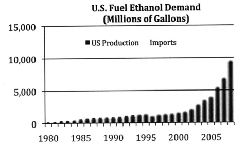
Ethanol has emerged as a near term fuel which has achieved scale to greater than any other alternative fuels, including fossil based alternatives like liquefied petroleum gas (LPG) and compressed natural gas (CNG). Ethanol is by far the largest non-petroleum alternative fuel (Davis 2008). While the environmental credentials are still a topic of debate, the use of ethanol is effective at simply displacing petroleum. The costs of deploying ethanol however are not trivial. The strategy of using ethanol as a fuel should be seen in the context of the multidimensional motivations that support its development. Commonly biofuels are treated as simply a greenhouse gas reduction strategy in policy. However the reasons more commonly used to support biofuels have to do with the domestic economic development and energy security arguments.

U.S. Fuel Ethanol Demand 15,000 (Millions of Gallons) N US Production Imports 10,000 5,000 0 1980 1985 1990 1995 2000 2005

Figure 1: Historic Ethanol Production in the United States and imports (Renewable Fuels Association 2008)

Course Correction

Transforming the vehicle and fuel fleet in the US is not a trivial matter. In the process of doing so, refueling infrastructure, vehicles and other existing systems must be altered. Biofuels and in particular ethanol offer hope as the largest non-petroleum based alternative fuel in the automotive market (US DOE: Energy Efficiency and Renewable Energy 2009). This type of success cannot be ignored.

However, there is a range of problems that emerge from the introduction of a new fuel system. The goal of this work is not simply to list the challenges, but to systematically explore the linked aspects of vehicle and fuel deployment in order to guide technology and policy

decisions over the next two decades.

The current biofuel mandates for the next decade include biofuel than can be used legally in gasoline blends if ethanol is used to meet the requirements. Section 211 of the Clean Air Act controls the addition of additives such as ethanol to limits that allow the blend to "substantially similar" pre-existing fuels. The interpretation of this statute has limited the legal blend of ethanol in gasoline to 10% by volume. Higher blends of ethanol, like E85, may only be sold to vehicles that have been certified by the manufacturer. However, there are not enough of these vehicles to use the high blends of ethanol that would be required to meet the original standards.

Additionally, there are not enough stations to distribute the fuel even if there were enough vehicles. Lastly, even with stations to distribute ethanol, and vehicles to use high blends of

the horizon, but none will scale in time to meet the current requirements. These combinations of factors leave US fuel policy in a position of pushing more fuels while phasing out incentives for the vehicles, which will use the fuel. The combination of these factors is increasing pressure to

certify higher blends of ethanol with uncertain consequences.

This research will systematically and quantitatively address each of the factors that present major obstacles to implementation of biofuels policy. It is hypothesized that coordinated policies along each factor; biofuels targets, ethanol blend limits, vehicle deployment, refueling deployment and customer purchase incentives will enable an effective transformation of the liquid fuel system to diversify away from petroleum sources of energy. The overarching question, which forms the foundation of this work, is how can benefits of ethanol be derived while minimizing the risks.

1.2.Scope

In this work, the focus is on the deployment of alternative vehicles, and specifically with matching the deployment of vehicles, fuels and infrastructure. Previous, and ongoing work by many research groups and organizations focuses on the environmental impact biofuels (Edwards, et al. 2006).

The net impact of a particular fuel or vehicle technology must be assessed across a broad scope of its impact. A life cycle analysis (LCA) has been utilized in understanding how vehicle emissions and fuel consumption vary with the addition of new technology. This technique is particularly important with the use of biofuels for transportation. In an LCA for automotive applications the impact of the fuel is typically called a well-to-wheels analysis (WTW). This can be further broken down into well-to-tank (WTT) which covers all the inputs that are used to make the fuel available for use, and tank-to-wheels (TTW) which refers to all emissions and effects from the utilization of the fuel (Edwards, et al. 2006).

This report will focus more on the TTW aspects of the biofuel system. As stated, there are challenges and opportunities regarding the use of ethanol that are not environmental. In this work the focus the technical and logistical impacts of ethanol and deployment of ethanol capable vehicles.

As ethanol blend percentages increase there are specific fuel properties that present the opportunity for improvements in efficiency and performance for light duty vehicles.

Understanding these improvements is important for guiding long term policy by fuel makers and distributers, auto manufacturers and government agencies.

The model results within the context of this research should not be viewed as predictions. The examples are meant to be illustrative examples of how various technologies and policies can overlap. Scenarios have been chosen for ease of understanding and relative simplicity. The lessons elicited should help bring better understandings of the fleet-wide interactions between vehicles, refueling infrastructure deployment and consumer demand.

1.3. Thesis Outline

There is a set of fundamental questions that will be addressed in this report. Each of these questions stem from variables in the following equation:

Equation 1: Total_ Biofuel(t) ~- Blendi% * Fleeti% * Utilizationi%

* Total Biofuel: The amount of biofuel used in the light duty vehicle fleet in a given year is dependent upon the following a set of proportions, each with additional embedded

factors. Biofuels are either ethanol or non-ethanol fully miscible alternatives.

* Blend Percentage: The component of fuel that contains blended ethanol. This factor is often represented as a volumetric percentage. E85 is used as the high blend of ethanol and E 10 or potentially E 15 may be used in the traditional gasoline supply.

* Fleet Percentage: There is a limited proportion of the fleet that is capable of operating on E85. While this value is calculated on a fleet basis, the fleet is an accumulation of new vehicle sales, which is the more common representation of market penetration.

* Utilization Percentage: For a given flex fuel vehicle, there is a choice of using E85 or regular gasoline. The utilization refers to how many vehicle miles are traveled using E85. The following chapters will explore in depth the issues that relate to each of these factors and how they impact the deployment of ethanol and ethanol capable vehicles.

Chapter 2: Fleet Model Methodology

The core analysis tool in this work is a model of all the cars and light trucks in the US fleet. Vehicles are separated by fuel type and assumptions are included for technological

development over time. Each of the following sections will specifically address an input area for parameters in the model.

Chapter 3: Total Biofuel (Policy & Availability)

The amount of biofuel used for blending is currently set as a matter of policy mandate. The Renewable Fuel Standard introduced in the 2007 Energy Independence and Security Act (EISA) will be the principal reference point for total biofuel targets in the US fleet context. However there are uncertainties regarding the amount and type of fuel that will be available. Therefore an assessment of the availability of feedstocks and maturity of fuel conversion technology will be included in the analysis for this chapter.

Chapter 4: Blend Level (Policy & Impacts)

Currently the legal limit for ethanol blends in gasoline is set at 10% by volume for conventional vehicles. This chapter will explore some of the considerations for increasing this limit to 15% by volume as well as address some of the basic fuel properties of ethanol that change as a function of blend percentage. For the purposes of this analysis there are effectively two types of fuel blends, those which can be used in the existing gasoline supply in any vehicle and a high blend of ethanol (E85) which can only be used in an FFV.

Chapter 5: Fleet (Deployment & Efficiency)

Chapter 5 lays out a set of FFV deployment scenarios, which can be used to better understand the requirements for meeting the total biofuels targets laid out in Chapter 3.

Additionally, there are design options for increased performance and efficiency in these vehicles based on the fuel properties discussed in Chapter 4. The analysis in this chapter will therefore

include a discussion of the amount and type of vehicles deployed and the effects within the fleet. Chapter 6: Utilization (Availability & Attractiveness)

The utilization value represents the percentage of FFV miles traveled on E85. This value is used as the output of the fleet model for all of the previous chapters. In order to translate these results into actionable policies it is important to understand the factors that are embedded in the utilization term. Utilization values can be achieved through a combination of fuel availability and fuel attractiveness. Availability is achieved through the conversion of retail fuel stations, and attractiveness is a function of price and vehicle performance on a given fuel. Chapter 6 includes a discussion of reasonable estimates for these values in order to test the reasonability of the existing deployment scenarios.

All of the previous chapters build up the support for selecting specific vehicle development scenarios while highlighting critical challenges and related issues. Ultimately this analysis can provide a set of recommendations for navigating the crucial tradeoffs that exist in the

2. Fleet Model Methodology

This chapter provides an overview of the methods and assumptions used to assess changes in vehicles and fuels in the US light duty fleet.

Foundations of the Model

The analysis tool at the heart of this research is a fleet model, which has been developed and refined by several researchers in the MIT Sloan Automotive Laboratory. The fleet model has multiple sets of input variables, which can be adjusted to achieve different scenario results. Previously it has been used to illustrate strategies for meeting fuel economy or greenhouse gas

targets (Cheah, et al. 2007). Detailed discussion of the model and relevant calibration can be found in "On the Road in 2035" (Bandivadekar, et al. 2008). While these variables are important for the behavior of the fleet dynamics, they are not the focus of this analysis. The existing fleet model was extended for the purposes of this analysis, to represent flex fuel vehicles as a vehicle class and to add E85 as an independent fuel.

The dynamics of fleet turnover are governed by a set of assumptions shown in Figure 2 and are used to formulate the baseline behavior of the fleet out to 2035. The average fleet fuel consumption improves over time based on a relative Emphasis on Reducing Fuel Consumption (ERFC). This concept has been described extensively by Bandivadekar et al. (2008). While the ERFC term includes strategies like weight reduction, there are additional light weighting strategies which can be pursued. Sales of cars and light trucks are treated separately and are assumed to retain fixed proportions.

REFERNCE CASE ASSUMPTION _{CARS LIGHT TRUCKS} New Vehicle Sales

Sales Growth 0.8% per year

Share of new sales that are light trucks ._55% Scrappage Rate

Median lifetime (years) 16.9 15.5

Vehicle Kilometers Traveled (VKT)

Starting VKT for 2000 Model Year 27,000 27,770

Degradation rate 4% 5%

Annual Growth in individual vehicle travel

0.5% (2005 to 2020) 0.25% (2020 to 2030) . . . .. 90 .1 % ( 2 0_ 3 -O_ t o 2 0 3 5 ) ,

On-Road Vehicle Fuel Consumption

A_____djustment Factor _22%

---Baseline Vehicle Mix (new vehicle sales in 2035)

NA PFI 2% 2%

Turbo 50% 50%

Diesel 9% 9%

Hybrid 30% 30%

PHEV 9% 9%

Emphasis on Reducing fuel Consumption 65%

Additional Vehicle weight reduction (0-35%) 17% Table 1: Fleet Model baseline assumptions

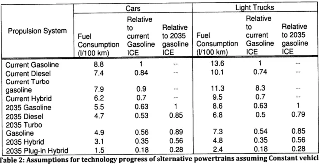
In order to make the output of the fleet model relevant for future policy makers it was assumed that CAFE regulations were met in 2020 with combined fuel economy of 35 mpg for combined cars and light trucks. The vehicle technology mix continues this trend to meet continuing stringency increases out to 2035. Each vehicle powertrain technology is assumed to have a level of potential for low fuel consumption shown in Table 2.

Cars Light Trucks

Relative Relative

Propulsion System to Relative to Relative

Fuel current to 2035 Fuel current to 2035 Consumption Gasoline gasoline Consumption Gasoline gasoline

(1/100 km) ICE ICE (1/100 km) ICE ICE

Current Gasoline 8.8 1 -- 13.6 1 --Current Diesel 7.4 0.84 -- 10.1 0.74 --Current Turbo gasoline 7.9 0.9 -- 11.3 8.3 --Current Hybrid 6.2 0.7 -- 9.5 0.7 --2035 Gasoline 5.5 0.63 1 8.6 0.63 1 2035 Diesel 4.7 0.53 0.85 6.8 0.5 0.79 2035 Turbo Gasoline 4.9 0.56 0.89 7.3 0.54 0.85 2035 Hybrid 3.1 0.35 0.56 4.8 0.35 0.56 2035 Plug-in Hybrid 1.5 0.18 0.28 2.4 0.18 0.28

Table 2: Assumptions for technology progress of alternative powertrains assuming Constant vehicle size and performance (Bandivadekar, et al. 2008).

The model takes inputs for the segmentation of new vehicle sales. Flex fuel vehicles are assumed to be an overlapping vehicle class. This means that all non-diesel powertrains are assumed equally likely to be FFVs. Diesel vehicles are considered with as a separate class of vehicles with separate fuel demand. FFVs retain the efficiency improvement each respective powertrain and may have increased fuel economy while operating on ethanol. This optimization assumption is set to zero in the reference case.

Ethanol is considered to be an "immiscible biofuel" in concentrations greater that 10% by volume (E10) unless otherwise stated. The criterion for miscibility is that special vehicle design is not required. Any biofuel that goes into the diesel supply would be considered to be a

"miscible biofuel" and would help meet the biofuel target but would not require the deployment of an FFV. Diesel biofuels are assumed to be miscible in the diesel fuel supply without requiring vehicle modifications.

Ethanol & Vehicle Analysis

The guiding framework for the model is based on Equation 1 in which the required volume of ethanol used in the vehicle fleet is considered as an input variable to the model in the form of the Renewable Fuel Standard. If this volume is less than or equal to the EPA blend

limit, then it is blended in the existing gasoline stock. However, when the mandated volume exceeds the legally allowable limit then the excess volume must be used in a higher blend of E85. The model includes an option to adjust the legal certification limit to E15 starting in 2012.

Additional inputs are used for the fleet sales percentage and the output of the model calculation is in utilization percentage as defined on the basis of miles traveled. This should not be confused with similar concepts such as percentage of total vehicle energy demand or percent of refueling events where E85 is used. Some of these subtleties will be discussed in Chapter 6.

Light Duty Vehicle

SFleet Penetration

3b i

FFV

[

Vehicle Distance Travelled: (Function of current year and year sold)

Vehicle Efficiency: (Based on percentage of technological potential)

Vehicle Attrition (distribution of vehicle lifetime)

Miles Traveled Miles Traveled on

on E85 Gasoline

Relative E85 _{Vehicle Mix PC}

KC

E85 Fuel Demand Ethanol Gas

i

I

EtOH

I

bta oline Usd Per

Ir

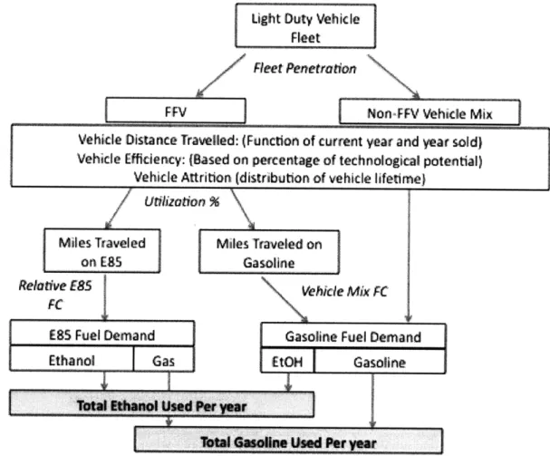
Figure 3: Updated fleet model structure for flex fuel vehicles (FFVs) showing the accounting approach for non-diesel vehicles. FC stands for Fuel Consumption, and EtOH is ethanol.

The breakdown of the model shown in Figure 3 is based on several key variables that determine the relative fleet composition and ultimate fuel use. These variables interact on the basis of the following general equation and internal fleet model mechanics:

Equation 1: Total _Biofuel(t) - CBlend,% * Fleeti% * Utilization ,%

* Fleet Penetration: Each scenario has a set percentage of new vehicle sales each year that are capable of running on E85. This segments the fleet into FFV and Non-FFV vehicles

* Utilization: A given flex fuel vehicle will only travel a certain proportion of miles using E85 as a fuel. This factor provides the breakdown between miles traveled on E85 and miles traveled on gasoline.

* Vehicle Mix Fuel Efficiency: The baseline vehicle sales mix is an aggregated composition of powertrain types. The combination of these and endogenous

technological development in fuel economy leads to the fuel requirement for a given set of miles traveled.

* Relative E85 Efficiency: Flex fuel vehicles have the capability of having increased fuel economy relative to the same vehicle operating on gasoline. This term is also referred to as FFV "optimization" which can be in the form of performance or efficiency as

discussed in Chapter 5.

* Blend Percentages: The fuel demand for blended gasoline and E85 each breaks down into a net demand for ethanol and gasoline. The blend proportions of ethanol in gasoline may change from 10% to 15% depending on the scenario.

The model uses iterative solving techniques to match utilization with a set of variables in each scenario. This utilization value is the minimum required to meet fuel mandates based on the existing vehicles, efficiency, biofuels target and other variables. The values of utilization used in the model for utilization are mostly meaningful within the range of 0-100%. Utilization greater than 100% would mean that the vehicle miles traveled (VMT) of FFVs would have to be greater than that of normal vehicles. This is not a meaningful result in the context of this study.

The model has the capability of solving for a solution to Equation 1 through two methods. In both cases the total fuel target and blend level are set.

1. National Deployment: Vehicle penetration scenarios are set, and the model solves for the

required utilization.

2. Regional Deployment: The utilization rate is set to a high value and the model solves for

the required new vehicle sales data.

The use of a high utilization rate simulates the localized deployment of dedicated ethanol

vehicles. This type of calculation shows a baseline for the minimum number of sales required as discussed in Chapter 5.

Baseline Fleet Performance

The fleet model leads to important changes in the vehicle technology mix and fuel consumption over the next 20 years. An important constraint on the model is that it meets CAFE standards that have been set for 2020. Part of the baseline assumption is that these standards continue to increase in stringency out to 2035. While these assumptions have an effect on the biofuel deployment these variables are not the focus of this work. The sensitivity of fuel use to the assumptions in Table 2 are discussed at length in "On the Road in 2035" and other reports (Cheah, et al. 2007). f H-160 140 120 100 080 0 60 0 1Feet 1970 1980 1990 2000 2010 2020 2030 45 40 35 (3 30 2 25 B 20 10 Cars 5 --- Light Trucks. - Fleet 1970 1980 1990 2000 2010 2020 2030

Figure 4: Baseline performance of the fleet model. Fleet fuel consumption is shown in billions of gallons broken out by cars and light trucks. Fleet average fuel consumption is shown in adjusted miles per gallon using a 22% adjustment factor from EPA fuel economy values.

It is critical to note that steadily increasing fuel economy is a part of the reference case in this model. Declining VKT growth and more efficient powertrains shown in Table 1 lead to a plateau and decline in total fuel used in the US LDV fleet. This means that fundamentally a constant volume fuel mandate will represent an increasing percentage of the total gasoline fuel supply. The following chapter will discuss potential scenarios for the available volume of biofuels.

3. Total Biofuel Targets: Policy & Production

This chapter will address two questions that are central to the fleet model scenarios: 1) What scale may biofuel production standards reach in 2035?

2) What types offuels are likely to be available to meet these standards?

3.1.Policy Context

The current ethanol market operates with near complete reliance on multiple policy measures. Nearly every policy tool is applied in some way towards ethanol production including taxes, subsidies and tariffs. The Volumetric Ethanol Excise Tax Credit (VEETC) went into effect in 2005 and is commonly referred to as the blender tax credit. Every gallon of ethanol is given this credit whether it is blended into ElO to provide $0.051 or E85 for $0.43 per gallon. Imported ethanol is subject to a $0.54 per gallon tariff in order to offset the tax credit. Many states also waive their excise gasoline taxes on fuel that has ethanol blended, particularly at higher volume concentrations (American Coalition for Ethanol 2008).

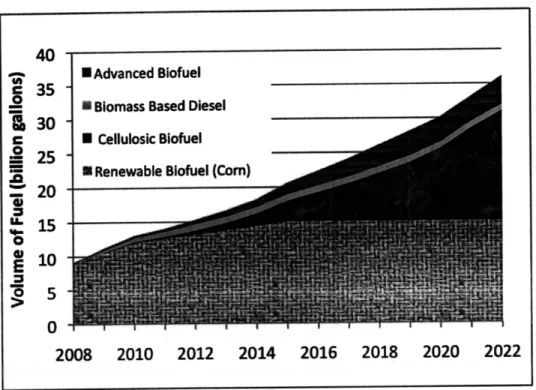
More recently, support for biofuel production has come from the Energy Independence and Security Act of 2007 (EISA), which included a significant increase in the Renewable Fuel Standard (RFS). The RFS states the total volume of biofuel that must be blended in the liquid fuel supply in a given year. Current blend requirements are ramping up to 36 billion gallons of renewable fuel by 2022. This renewable fuel mandate replaced the previous version from EPACT 2005, which peaked at 7.5 billion gallons in 2012 (Cong. 2005).

40

- I Advanced Blofuel

c 35

l

Biomass Based Diesel

30

2C i Cellulosic Biofuel

SRenewable Blofuel (Corn) 20

-15

-10

0

2008 2010 2012 2014 2016 2018 2020 2022

Figure 5: Renewable Fuel Standard contained within the 2007 Energy Bill (EISA). Total biofuels reach 36 billion gallons per year in 2022 with corn ethanol limited at 15 billion gallons and 22 billion gallons of biofuel achieving at least a 50% Life cycle benefit against a 2005 petroleum baseline. No less than 1 billion gallons of this may be biomass-based diesel after 2012. 16 billion gallons out of the 22 are cellulosic biofuels must achieve 60% life cycle GHG benefits.(C. United States 2007).

The RFS mandates shown in Figure 5 are made on a volumetric basis and segmented on a life cycle greenhouse gas (GHG) reduction against a gasoline baseline. Official life cycle

assessment (LCA) techniques have not been set at this time been set, but the EISA explicitly states that land use change must be considered. This is a highly contentious issue, which has the power to drastically affect the way that fuels will be viewed for this policy. The amount of corn based renewable fuel is limited to 15 billion gallons. Some amount of biofuel must come from feedstocks defined as cellulosic, while the remaining volume may be non-specific biofuel as long as it meets the LCA requirements of 50% benefit against baseline. There is no explicit mention of the type of fuel that must be produced except the provisions for biomass-based diesel, which

grow to a minimum of 1 billion gallons. The bill stipulates that while economic hardship can lead to the reduction of the mandate if the fuel is not available, that the proportions of cellulosic to corn ethanol must remain the same.

The scale and timing of the RFS mandates create a situation where it is unlikely to be successful in the exiting policy framework. The current legal limit for blending remains at 10% by volume. However, in the next few years it is virtually certain that the current Renewable Fuel Standard will exceed this legal blend limit. The term "blend wall" has been used to describe the

situation when more fuel is mandated than can be blended in gasoline. The EPA has announced for 2009 that the blending requirements are 10.21% (US EPA 2008). The standard applies to the continental US with opt-in available for Alaska and Hawaii, which Hawaii has chosen to do. Small refiners are exempt from the requirements until 2011, which account for 13.5% of total fuel production. Once the total amount of fuel covered by the RFS increases in 2011 the volumetric requirements will result in a smaller blend percentage. It is clear, however, that the blend wall is a near term problem and is likely to impact fuel distribution within the next 3-7 years. In order for the entire RFS volume in 2022, estimates show that ethanol blends greater that 20% would need to be used in all gasoline. Figure 6 below shows an illustration of the required blend level that would be required in order to extend the blend wall.

40

RFS Blofuel taret

1 30 --- ...

-Elp Blend Limit

I | -0 ...--- ---...- r-1 r-10r-1 --- LILI1-- --- --- --- r-- --- --- t SI 2010 2015 2020 2025

Figure 6: Illustration of the blend wall issue assuming no E85 use. The E10 blend limit is the amount of ethanol that could be used to meet the RFS requirements if all gasoline included 10% ethanol. The E15 blend limit occurs when all states blend 15% ethanol in all gasoline. The blend limit lines are shown for the highest possible value assuming no decrease in total fuel use.

Thus far, the EPA has denied waiver requests to reduce the RFS (US EPA 2008). There is some question as to whether or not the RFS will be attainable in 2022. Current policy continues to drive towards increasing volumes of ethanol production. However, the implementation of these policies may be tempered by the availability of fuel. The next section will explore the production of biofuels. At the end of this chapter both the policy and technology aspects of biofuel targets will be combined to generate scenarios for use in the fleet model simulation.

3.2.Production of Biofuels

It is still uncertain which types of feedstocks and fuels are most likely to meet the RFS requirements in the US. There are three major factors that can be used to reach a better understanding of total availability of biofuels. These are:

* Conversion Technology: The technology that is used will determine what types of fuels can be made. However conversion will rely on specific types of feedstocks. Capital intensity and technological complexity will also determine scalability.

* Biomass Resources: The feedstocks will determine geographic distribution, carbon intensity with a strong feedback into the scalability.

* Scalability: The combination of the first two factors with a consideration for cost competitiveness will constrain the proliferation of biofuel production.

There is a strong interplay between each these factors. Biomass resources can be considered as long as there is viable conversion technology to convert the feedstock into fuel. The combination of feedstock costs and process efficiency leads to a general cost

competitiveness, which may then feedback into the selection of feedstocks and fuels. It is valuable to address each of these topics to ascertain reasonable estimates of how much of which type of biofuel will be available and when. The US biofuels market is dominated by ethanol, and domestic ethanol is made almost exclusively from corn (Wright, et al. 2006). The more

important question for meeting future RFS targets is how the cellulosic fuels will be made. For advanced biofuels there are three basic categories of biomass conversion (Sandia National Labs, GM R&D Center 2008).

1. Biochemical: These processes are catalyst by microorganisms, which carry out fermentation reactions. Cellulosic materials can be broken down by specific enzymes or by redesigned bacteria.

2. Thermo-chemical: Inorganic catalysts are used along with high pressures and temperatures to break down cellulosic material. Then catalytic synthesis is used to create different types of fuels.

3. Biochemical/Thermo-chemical: There are options to combine these two processes by first gasifying cellulosic feedstocks and then using the gas as a feedstock for biological fermentation

The cellulosic ethanol plants that are being planned and developed today are the best resource for understanding the type of fuel processes which will be first to scale up. The data for understanding the biomass resources and conversion technology maturity comes from an

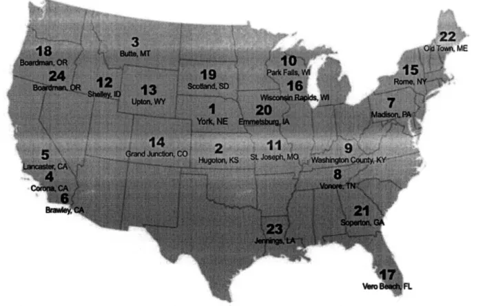
accumulation of press releases from companies, and also from the US Department of Energy (DOE), which has provided loan guarantees to some of the biofuel producers. Figure 7 below shows a map of the locations for proposed cellulosic ethanol projects in 2008 numbered from 1-24 corresponding to values in the Appendix. Some projects have been cancelled, and others have been added from the time of this assessment.

Figure 7: Geographic representation of cellulosic pilot plants in planning or construction phases. (Renewable Fuels Association 2008)

All of the proposed pilot facilities share the goal of scaling up production to meet the RFS mandate for cellulosic biofuel. However, the pilot scale is usually on the order of 25,000 gallons per year while commercial scale for corn ethanol production facilities is around 100 million gallons per year. Ultimately the RFS target is 16 billion gallons in 2022, which means that plant scaling must happen relatively quickly (C. United States 2007). The currently planned cellulosic facilities will need to scale to 100 million gallon annual capacity by 2015 in order to meet the RFS requirements The RFS continues to grow after 2017 at the same rate. The

development of cellulosic plants will also depend on the biomass feedstocks, which will be used in the fuel conversion. Based on the current rate of progress for cellulosic plants it can be

reasonably expected that some of the RFS target volumes for cellulosic biofuels will not be met. Additionally, this shows that the current technology, though somewhat varied is almost

exclusively for the production of ethanol. The lack of near term evidence of scalability for other fuels is an indication that commercial production will continue to lag that of ethanol.

Feedstock Resources

The deployment cellulosic ethanol fuel relies on biomass feedstocks for conversion. The type of feedstock will play a role in the total amount of fuel that can be produced, the location of production, and the type of fuel. For these reasons, an overview of potential feedstock options is warranted. There are four basic types of biomass resources that will be discussed here. Each feedstock becomes enabled as processing and conversion technology develops, and has particular challenges to overcome.

Phase 1) Traditional Agricultural Products

Corn ethanol has been and continues to dominate US biofuels. Current corn ethanol production is projected to reach 10 billion gallons per year by 2010. Corn Planting Acreage has

stayed relatively steady around 80 million acres while the number of bushels per acre has continued to climb steadily past 150. With continuing conversation rates of 2.7 bushels per gallon, 15 billion gallons of ethanol from corn is reasonably achievable using 30% of the corn crop and continuing technological improvement in yield and conversion rates. Approximately 90 Million tons of corn are used in the United States today, and industry average conversion is

around 200 L per metric ton. Ethanol can present modest life cycle benefits in GHGs but also interferes with existing agricultural activities and can stress water and fertilizer use. (Groode 2008)

Phase 2) Agricultural & Industrial Residues

The production of corn and other traditional crops generates additional biomass that is not used. The increase in corn planting acres comes with a corresponding increase in the

availability of corn stover. This is a cellulosic feedstock that requires special treatments, but allows for the co-location of new cellulosic ethanol plants next to existing plants without major changes in supply chain. Roughly half of the dry tonnage per acre for corn results in unused residue. Estimates from 2001 put total crop residues at nearly 500 million dry tons per year out

displace fertilizer requirements by returning nutrients to the soil. USDA Estimates of the actual availability of corn stover specifically are closer to 100 million dry tones (US Department of Agriculture 2007).

The next largest available source of crop residues would be from soybeans, which provides more than 100 million dry tons per year with 50% removal. Total assessments of the resources from sustainable harvest are as high at 368 million dry tons per year from the

combination of various agricultural residues. Many of these residues are already used for existing energy resources such as co-firing (Wright, et al. 2006).

The second type of cellulosic residues come from the forestry and paper industries. There are abundant woody biomass references from urban sources such as construction and demolition.

Collection and processing mechanisms have not yet been well established for many of these residues. The heterogeneity of some feedstocks also presents a challenge for processing biofuels. Phase 3) Dedicated biomass feedstocks

Several different types of energy crops have been proposed, ranging from fast growing strains of prairie grasses, to woody feedstocks such as poplar or miscanthus. In many cases the growth of energy crops is proposed on Conservation Reserve Program (CRP land). There will be some price at which farmers might switch corn-planting acres to grow switchgrass. Analysis by Groode (2008) also includes a measure of the capacity of CRP land. The management of these lands will play a role in how much dedicated feedstocks may be deployed for biofuel production. Phase 4) Potential new types of farming resources

After agricultural products, residues, and dedicated fuel crops there are other non-traditional feedstocks that have been proposed. Algae biofuels are the primary example in this category. Algae as a feedstock is still in the early phases of exploration but presents some promise for use as a source of bio-oil for biodiesel. Algae represent an opportunity for decreased land use, but still have significant water and capital requirements to create a viable production system (Sims, et al. 2008).

Total Available Biomass

There have been several studies over the past two decades looking at he availability of biomass, and there are general assumptions that must be made at each point. Many of the studies suggest that hundreds of millions of tons of biomass are obtainable in a sustainable manner (U.S. DOE, USDA 2005). For example BP has estimated that biofuel could account for 10-30% of the global transportation fuel market by 2030 (Ellerbusch 2008). Similarly, Sandia National Labs in

partnership with GM suggest that the volumes of 60 billion gallons of ethanol could be produced by 2030 (Sandia National Labs, GM R&D Center 2008). Others, however, warn of major

environmental damage that can result from expanded biofuel production (Melillo, et al. 2009). Based on current trends it is likely that agricultural crops will continue to play a large role, but feedstocks will begin to expand into waste steams and move towards dedicated energy crops as the value increases. The general assessment is that there is enough biomass to support continued growth of biofuel development. However, growth of this industry will be constrained by logistics in managing the biofuel supply chain as well as competition between biofuels as well as against traditional fuels.

There are increasingly studies that delve into the issues of supply chain logistics and sourcing biomass to conversion facilities (University of California, Davis 2008). However, there is evidence to suggest that the total availability of biomass is not the limiting factor for existing biomass targets. The constraints will be on what can be economically recovered and converted. Fuel Types, Maturity & Market development

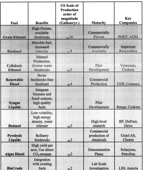
While there are many types of biofuel under development, there are few that have been able to reach large scale and widespread deployment. Table 3 below shows a broad assessment of the various types of biofuels that are currently being produced and the level of production maturity that has been achieved. There are essentially three phases that emerge: the large-scale commercial developments, pilot plant stage developments, and lab scale technology

development. There is still significant stratification within each class shown by the changing orders of magnitude of production. This is not an exhaustive list, but provides some assessment of the range of options that are currently under investigation. Additionally, new projects are emerging to advance the development of each fuel.

Table 3: Production of various biofuels divided up in to commercial, pilot and R&D stages (adapted and augmented from (National Renewable Energy Laboroatory 2006))

While ethanol and specifically that which has been produced from corn has attained early market leadership, there is a range of other fuels, which are prepared to compete with corn

ethanol. The landscape of biomass feedstocks and conversion technology is dynamic and intricate even only addressing the basic factors above. Fundamentally there is a sequence of developments for each technology to reach scale, which are not trivial. Corn ethanol technology

has existed for decades but is still not cost competitive with recent gasoline prices without heavy subsidization.

The assessment in this chapter thus far has provided an overview of the existing biofuels policy as well as emerging options for future fuel feedstocks and formulations. These variables

can now be assembled into representative scenarios in the final section of this chapter.

3.3.Scenario Analysis: How Much of What, and When?

The biofuel policies in the US are currently based on the Renewable Fuel Standard as described in the beginning of this chapter. However there are two key areas of uncertainty in the application of this mandate through 2022 and out to 2035.

1) Total amount of biofuels mandated by year.

2) Type of fuels that will be used to meet this standard

A complex landscape of fuels, feedstocks and technologies is emerging, and it is not clear how the competition between biofuels will play out through 2035. There is also some doubt regarding the specific policies that will support biofuel production. In order to deal with these uncertainties in the context of the fleet model, a range of possible future scenarios must be explored. While the RFS, as written, can be taken as a baseline through 2022 there are reasonable doubts that these targets will be met, especially given the current state of

development for cellulosic pilot plants. Additional support for seeing the RFS targets delayed comes from the EIA Annual Energy Outlook.

The EIA reference case, projects a slight delay with RFS goals met in 2027 instead of 2022. In the long term scenario for 2030 biofuel production continues to increase. The EIA scenarios are not meant to serve as forecasts, but can be useful as baseline scenarios for comparison. (EIA 2009)

In the case of rapid technological development and high gasoline prices, it may be possible for biofuel mandates to continue growing. Based on the range of assessments a set of possible future biofuel targets were assembled. These include the following cases:

* Reference Case: The current RFS, with increasing cellulosic targets to reach a total biofuels targets of 60 billion gallons in 2035.

* Delayed RFS: A three-year delay in cellulosic targets with an eventual achievement of the original RFS targets in of 36 billion gallons 2035. Any additional growth in cellulosic fuels is used to displace corn ethanol.

Both cases can be represented with the development of non-ethanol biofuels that would be legally miscible in the gasoline supply. This would include products like butanol or a biosynthetic gasoline fuel. In this case the assumed penetration is that 50% of the cellulosic fuels component becomes the miscible alternative. The mix of cellulosic and corn ethanol does not effect the deployment of FFVs, but will change the net GHG intensity of the fuel mix, and may allow for the use of unconventional oil resources. The two major fuel scenarios are shown

in Figure 8. Each scenario includes a second option for the inclusion of non-ethanol miscible biofuels. This type of fuel is assumed to contribute to meeting the fuel requirements without

requiring any vehicle modifications or blend limits.

High Fuel Scenario - Extended RFS Low Fuel Targets - Delayed RFS

80 '(Billions of Gallons) 80 (Bilonso)s

60 .. Non-Ethanol MisciblI Fuel. 60 Non-Ethanol Miscible Fuel

Cellulosic Ethanol Cellulosic Ethanol

40 Corn Etha no 40 Corn Et-hano

0 0

2010 2015 2020 2025 2030 2035 2010 2015 2020 2025 2030 2035

Figure 8: (left) The high target fuel scenario reaches the existing RFS targets of 36 billion gallons of biofuel 2023. This trajectory continues to reach 60 billion gallons total in 2035. Here the scenario is shown with 50% penetration of non-ethanol miscible fuels. The scenario is also run with a minimum of 1 billion gallons of miscible biofuels. (right) The low fuel target scenario is shown with existing RFS targets reached in 2035. Additional growth in cellulosic ethanol is used to displace corn ethanol. This graph is also shown with the option addtion of miscible fuels. The baseline case includes only 1 billion gallons of miscible biofuels.

These two cases represent an aggressive and conservative estimate respectively of the potential biofuel development. In all further discussion these two scenarios will be referenced as the high fuel case and the delayed RFS case for biofuel targets. They effects of changing

between the high and low fuel targets on utilization is shown in Figure 9. The baseline FFV deployment scenario is used which includes a linear market penetration leading to 50% of new vehicle sales in 2035.

100%

90% _{High Fuel Target}

80% -70% 60% Delayed RFS 50% 20% -- -- -- --- ---0% 20%10 2015 2020 2025 2030 2035 10% 0% 2010 2015 2020 2025 2030 2035 100% S90% .- H-

i.---80% - High Fuel Target

S80%

0 70%----

---o 60% ---- -

---=50% _40%

---

High Fuel Target

30%

- with Miscible fuels

S_{20% - ----}

---0%

2010 2015 2020 2025 2030 2035

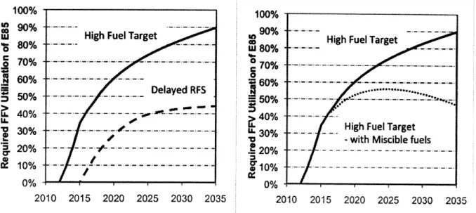
Figure 9: (left) The required utilization is shown for reference deployment levels of FFVs reaching 50% of new vehicle sales in 2035. The effect of changing scenarios from the high fuel target of 60 billion gallons in 2035 to the delayed RFS achieving 36 billion gallons in 2035. (right) The same scenario assumptions are shown with the addition of non-ethanol miscible fuels to the high fuel target scenario.

There are two fundamental types of shifts that occur based on the changes in fuel targets and fuel composition. Delaying the RFS targets shifts the date at which utilization increases begin, and also reduces the total maximum utilization required. There is an additional effect whereby the same volume of ethanol requires a lower utilization rate. 36 Billion gallons of fuel requires a utilization of nearly 70% in 2023, however in 2035 it is only 45%. This decrease is due to the continual build-up of FFVS in the fleet, which spreads the utilization requirement over a greater number of vehicles.

The gradual introduction of non-ethanol miscible fuels decreases the utilization

requirement for FFVS over time by reducing the amount of ethanol that must be used. In each case there may be an additional effect from the introduction of non-ethanol biofuels. These may be diesel, or a synthetic gasoline. The same effect can be achieved by reducing the biofuel targets if ethanol is the only biofuel available.

For a given vehicle deployment scenario all fuel scenario options can be plotted on the same graph. There are two total fuel targets, and each target includes the option for a separate fuel mix. The combined results for baseline FFV deployment are shown in Figure 10 These four cases can be plotted together to better understand the relative impacts of each. This graph shown

in Figure 11 will be revisited in successive chapters to show how additional policies effect utilization.

Required Utilization

%

for all FFVs

100%0

Blend: E10 maximum ethanol in gasoline

90% _{FFV Sales: Baseline reaching 50% in 2035} 80%

70%P---(A)

60% - - - - -

-50%High

fuel target -60 Billion gallons of ethanol required in 2035 (B) High fuel target with the introduction of miscible biofuel _{4 0 %} Low fuel target reaching 36 billion gallons in 2035 (D) Low fuel target with the_{-- ---. .} (C). _{-- - -- - -- - - .... . ... . . . .}

30%is due

to the combined effects of delayed targets, decreased ethanol fuel and accumulation of

_IN5

_--

---20% -- - - -- - -

----10% ....--- ---

--10%

----4---2010 2015 2020 2025 2030 2035

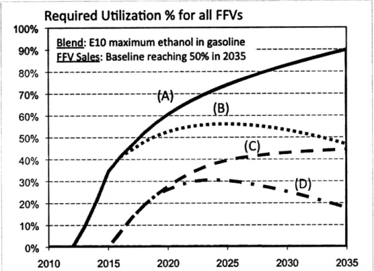
Figure 11: Combined results for utilization requirement of FFVS to meet all four fuel scenario targets (A)

High fuel target - 60 Billion gallons of ethanol required in 2035 (B) High fuel target with the introduction of miscible biofuel (C). Low fuel target reaching 36 billion gallons in 2035 (D) Low fuel target with the

introduction of miscible biofuel.

The relative effect of adding miscible biofuels has significant impact in both cases. It is notable that in the delayed RFS case the required utilization actually falls in the later years. This

is dues out tohe combined effects of dominane in biofuels will likecreased ethanol fuel and accumulation of capable vehicles in the fleet. The effects of reducing utilization requirements are counter-balanced by an overall decrease in total fleet fuel consumption.

The standards for biofuel production are based on a set volume amount, but the blend limits are on a percentage of fuel used. This means that the decreasing total fuel consumption, shown in Chapter 2 for the baseline case, makes biofuel targets more difficult to meet in terms of utilization. The baseline fleet scenario represents a more challenging case for later years because of continual improvements in fuel economy.

The dominant alternative fuels for transportation in the United States will likely continue to be ethanol over the next 15 years. There is potential for ethanol to reach steadily increasing volumes out to 2020. Ethanol dominance in biofuels will likely be challenged by the emergence

of other advanced biofuels that may prove easier to blend with conventional fuels. The

percentage blend percentage of ethanol in gasoline and E85 will therefore depend on the type of biofuels available and the total fleet fuel use of the US LDV fleet at that time. The following chapter will address many of the issues that emerge from varying blends of ethanol in gasoline.

4. Blend Levels: Fuel Properties & Policies

This chapter will address the types of ethanol blends, which are likely to be available, and the fuelproperty concerns that exist with these blends. Understanding the positives and negatives of ethanol as a blend component is critical to evaluating the future utility and desirability of ethanol. This chapter forms the foundation of chapter 5 by identifying aspects of ethanol which effect vehicle performance, as well as setting up the scenario assumptions for legal blend limits.

Fuel policy regarding ethanol can be a very contentious issue because the impacts cut across several different areas of concern for multiple stakeholders. It is valuable to begin with these concerns because the addition of ethanol will provide some combination of opportunity and risk to each stakeholder. The net balance of benefits against costs will factor into the amount of resistance to ethanol policies.

There are major industries involved in each step of the value chain that relates to ethanol introduction. Feedstock producers, ethanol producers, refineries, distribution systems, retail fuel stations, automakers, drivers, and the government all have reason for concern regarding how ethanol is introduced as a transportation fuel. Due to the interconnected nature of the entire fuel value chain each group must also be concerned with the concerns of the end user of the fuel. The degree of concern also varies, but the main point is that there are a range of fuel properties that change significantly with the addition of ethanol and that this impact can be felt in different ways by all stakeholders in the fuel system.

The reason for concern varies by stakeholder group, but for most it is the result of the interaction with some existing fuel policy or a matter of performance. The following sections will discuss some of the tradeoffs that exist in blending ethanol into gasoline.

4.1.Fuel Policy Overview

The blend wall limit, discussed in Chapter 3, exists at the current maximum of 10% ethanol. Attempts to increase the amount of ethanol fuel sold can be achieved by increasing the

blend level in the fuel supply. Blends can increase in an incremental fashion by increasing the E10 blend limit to E15 and E20, or by increasing the sales of high blends like E85. However, as recently as 2005, E85 only accounted for 1.2% of ethanol sales in the US (Davis 2008).

The core questions with respect to blending is whether or not mid level blends of ethanol such as E 15 or E20 should be certified by the EPA as a replacement fuel. Recently, the state of Minnesota has sought a waiver for E20 blends and more recently a coalition of ethanol producers has requested a waiver for E15 (Growth Energy on Behald of 52 US Ethanol Manufacturers 2009).

A new fuel blend will lead to risk for existing vehicles that may see impacts in emissions, drivability and warranty concerns. The certification of E15 creates an issue where government agencies are put in the position of deciding whether or not a vehicle can operate outside of its originally intended fuel use. Even if E 15 is certified as a fuel drivers may not choose to use the fuel if the manufacturer does not recommend using E 15.

Another key gating items for the certification of E 15 is challenge of adaptability in the current infrastructure. Recently Underwriters Laboratories (UL) has agreed to use the UL 87 certification towards fuels containing ethanol blends up to 15% (Underwriters Laboratories 2009). There are no clear answers yet although; extensive work is underway by the DOE to examine whether or not E 15 can be used as a direct fuel replacement.

Regional Policies for Vapor Pressure

The blend level of ethanol affects many other fuel properties, which are currently regulated. One particular example is the vapor pressure of gasoline fuel. There are standards drawn for the US based on spatial and temporal dimensions. Northern states may have higher vapor pressure because of the tendency towards lower temperatures. Similarly, there are seasonal blends along two seasons, which have lower vapor pressure in the summer and higher in the winter. During the period of June through September 15 the maximum RVP is 7.8 psi in southern states. In the rest of the country the maximum is 9.0 psi. There are additional, state-specific low vapor pressure programs. These regional policies may require 7.8 or lower RVP (Marathon Oil Corporation 2008).

The adjustment in fuel volatility also aids cold start operation. If fuels are not volatile enough it can lead to increased hydrocarbon emissions during startup if the fuel is not fully vaporized. Certain urban areas have been designated ozone nonattainment zones by the EPA,

where there are specific requirements for reformulated gasoline to have a VOC reduction of 20-25%. This may also be coupled with a vapor pressure or ethanol requirement. One of the most

contentious policy issues has been the issuance of a ipsi waiver ethanol blends between 9-10%. Initially the EPA denied this waiver, but strong pressure from the ethanol industry reversed this decision. Some environmental groups teamed up with the oil industry in opposing the waiver (Segal 1993).

Variability in Blends

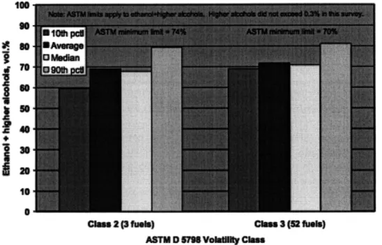
Common terminology is used to represent ethanol blends such as E 10 for 10% ethanol and E85 for 85% ethanol. However there is inherent variability in these blends due to seasonal variations and blending techniques. When ethanol is first distilled and filtered to become 100 % ethanol is must be denatured to avoid taxation as liquor(Alcohol and Tobaco Tax and Trade Bureau 2008). Typically pure ethanol is blended with 2-5% gasoline as a denaturant. This means that the ethanol used for blending begins as E95 and therefore E85 typically contains 80%

ethanol. However this can be much lower in the winter due to changing vapor pressure

requirements. The Coordinating Research Council (CRC) conducted a survey of commercially available E85 in the winter to test the actual concentration of ethanol. The results are shown in Figure 12 which indicates that actual blends may be as low as 60 or 70% for part of the year despite being labeled as E85 (Coordinating Research Council 2007).

MTaM DUR vogla Cl..m

Figure 12: Results from a CRC study of 15 states for winter blends of E85 (Coordinating Research Council 2007).

The method of blending also can have an impact of the fuel properties of the mixture. Splash blends use existing gasoline feedstocks. While specialty blends of ethanol can utilize lighter fractions of gasoline to balance out the vapor pressure of ethanol. The location of blending will also determine other fuel properties. For example if 87 octane is blended with ethanol the then consumers buying E 10 regular will actually get higher octane fuels. Currently the energy content of fuel is not labeled.

4.2.Fuel Property Overview

Gasoline as a fuel consists of many different compounds, the proportions of which are finely tuned in the refining process to achieve fuels that perform well, within existing cost constraints. Ethanol is a single molecule and therefore has constant properties, but does exhibit some nonlinear trends as it is blended with gasoline. The effect of ethanol blending on gasoline fuel properties will determine which blends are most suitable for use and will guide the design of refineries, distribution networks and vehicles.

Fundamental properties of ethanol and gasoline can be compared in Table 4, and will be used for reference in the rest of this work. It is important to note that there is variability

especially in the values for gasoline since there are many types, grades and composition factors. While the values for ethanol are more consistent the blends of ethanol and gasoline can exhibit very different qualities. The volumetric energy density is perhaps the most important value since it will be used in later calculations. For the purposes of this work ethanol is considered to have 66% the energy in gasoline on a volumetric basis.

Fuel Property Ethanol (E100)

I

Research Octane Number (RON) 108 90-100

Specific Gravity (kg/1) 60F/60F 0.79 0.75 Net Heat of Combustion (LHV) MJ/kg 27 43 Net heat of Combustion (LHV) MJ/I 21 32

Stoichiometric air/fuel ratio 9 14.6

Reid Vapor Pressure (RVP) psi. 2.3 8-15

Table 4: Fuel Property overview for ethanol and gasoline.

Molecular Composition

Ethanol is different from conventional hydrocarbons in several ways. One of the key differences is the oxygen content. Ethanol is also partially oxidized relative unlike other

hydrocarbons, which results in lower energy content. The partial oxidation however also means that less oxygen is required in combustion which leads to a lower gravimetric air to fuel ratio. However, due to the change in energy density, the air required at a given engine load is roughly the same for E85 (Wittek, Tiemann and Pichinger 2009).

The molecular composition of the fuel is measured by the percentage composition of hydrogen, carbon and oxygen. While oxygen relates to the amount of air needed, the H:C ratio is a way of determining emissions in the fuel. Shorter chain saturated hydrocarbons have a higher H:C ratio than longer chain hydrocarbons. This means that in complete combustion fewer carbon products are formed from the fuel. Ethanol produces a slightly lower amount of C02/MJ of fuel burned than gasoline just based on its molecular composition. Further improvements are possible based on efficiency differences between the utilization of the fuels, which will be discussed in Chapter 5.

Energy Content

Ethanol by itself contains approximately 2/3 the energy content of gasoline on a volumetric basis. The total energy content scales linearly with the volumetric percentage of ethanol as shown in Figure 13. Blends of E85 typically contain 70-80% of the energy per unit volume when compared to regular gasoline.

50

0 20 40 60 80 100

lume fraction of no in gaoline %]

Figure 13: Relative energy as a function of ethanol blends in gasoline (Wallner and Miers 2008).

The practical effect of having less energy per volume means that fuel injectors must deliver a greater amount of fuel at a given engine load. The effects the size and calibration of the injectors over the range of operation and is a contributing factor in the needed specialization of flexible fuel vehicles.

For constant energy efficiency and volume of fuel tank, a lower energy density means more frequent refueling. Increased fuel purchase means more expense unless the cost is

equivalent per unit energy. Ethanol blends typically sell for less per gallon than gasoline, but are