HAL Id: tel-01652369
https://hal.archives-ouvertes.fr/tel-01652369
Submitted on 30 Nov 2017
HAL is a multi-disciplinary open access archive for the deposit and dissemination of sci-entific research documents, whether they are pub-lished or not. The documents may come from teaching and research institutions in France or abroad, or from public or private research centers.
L’archive ouverte pluridisciplinaire HAL, est destinée au dépôt et à la diffusion de documents scientifiques de niveau recherche, publiés ou non, émanant des établissements d’enseignement et de recherche français ou étrangers, des laboratoires publics ou privés.
shape gradient and Level Set method
Zhidong Zhao
To cite this version:
Zhidong Zhao. Planar antenna and antenna array optimization by shape gradient and Level
Set method. Electromagnetism. Université de Nice - Sophia Antipolis, 2015. English. �NNT : 2015NICE4097�. �tel-01652369�
UNIVERSITE DE NICE-SOPHIA ANTIPOLIS
ECOLE DOCTORALE STIC
SCIENCES ET TECHNOLOGIES DE L’INFORMATION ET DE LA COMMUNICATION
T H E S E
pour l’obtention du grade deDocteur en Sciences
de l’Université Nice Sophia Antipolis
Mention : Electronique
présentée et soutenue par
Zhidong ZHAO
Optimisation d'antennes et de réseaux d'antennes planaires par
gradient de forme et ensembles de niveaux (Level Sets)
Planar antenna and antenna array optimization by shape gradient
and Level Set method
Thèse dirigée par Christian PICHOT
Soutenance prévue le 23 Novembre 2015
Jury :
M. Matteo PASTORINO Professeur, Université de Gênes, Italie Rapporteur
M. Giuseppe PELOSI Professeur, Université de Florence, Italie Rapporteur
M. Ala SHARAIHA Professeur, Université de Rennes 1 Examinateur
M. Claude DEDEBAN Ingénieur, Orange Labs Examinateur
TABLE OF CONTENTS
CHAPTER 1: INTRODUCTION ... 1
1.1 Antenna analysis and design ... 3
1.2 Antenna optimization algorithms ... 3
1.3 Topological Gradient and Level Set method ... 4
CHAPTER 2: ELECTROMAGNETIC THEORY ... 6
2.1 General Questions ... 7
2.2 Maxwell Equations ... 7
2.3 Boundary Conditions ... 8
2.4 Wave Equations ... 9
2.5 Surface Equivalence Theorem: Huygens Principle ... 10
2.6 Radiation condition ... 11
2.7 Green’s Function ... 12
2.8 EFIE and MFIE Equations Definition ... 12
2.9 Reaction Concept ... 14
2.10 Variational Formulation ... 15
CHAPTER 3: SR3D ... 17
3.1 Linear system ... 18
3.2 Reaction Matrix Z ... 19
3.3 Source Vector Definition ... 24
3.4 Reaction Matrix Discretization ... 26
3.5 Source Vector Discretization ... 28
CHAPTER 4: OPTIMIZATION TECHNIQUES ... 30
4.1 Global and local optimization ... 31
4.2 Stochastic method ... 32
4.2.1 Genetic Algorithms ... 33
4.2.2 Particle swarm optimization ... 33
4.2.3 Simulated annealing ... 34
4.2.4 Ant colony optimization ... 34
4.3 Deterministic method ... 34
4.3.1 Shape gradients calculation ... 35
4.3.2 Shape optimization using shape gradients ... 35
CHAPTER 5: SHAPE GRADIENT ... 37
5.1 Discrete method ... 39
5.2 Adjoint method ... 40
5.3 Analytical method ... 40
5.4 Shape gradient based on topological deformation ... 46
5.4.1 Contour definition of shape geometry ... 46
5.4.2 Shape Gradient method using nodal point mesh derivation ... 48
CHAPTER 6: LEVEL SET METHOD ... 53
6.1 General Description ... 54
6.2 The Level Set Function ... 54
6.3 The Normal Velocity ... 56
6.4 The Narrow Band method ... 58
6.5 Re-initialization ... 59
6.6 An upper limit to the size of Δt ... 60
6.7 Apply shape gradient to Level Set method ... 61
6.8 Procedure of Level Set optimization ... 62
CHAPTER 7: NUMERICAL VALIDATIONS ... 63
7.1 Study of the scattered field of a cylinder antenna ... 64
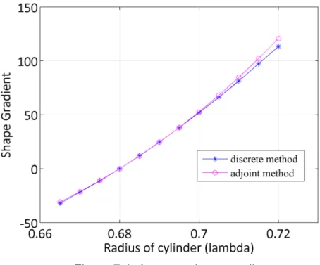
7.2 Validation of the adjoint formula for a cylinder antenna ... 68
7.3 Validation of the adjoint formula for a 2D patch antenna ... 70
7.4 Validation of the adjoint formula for a 3D patch antenna ... 73
7.4.1 Thin 3D patch antenna enlarging along all normal direction ... 73
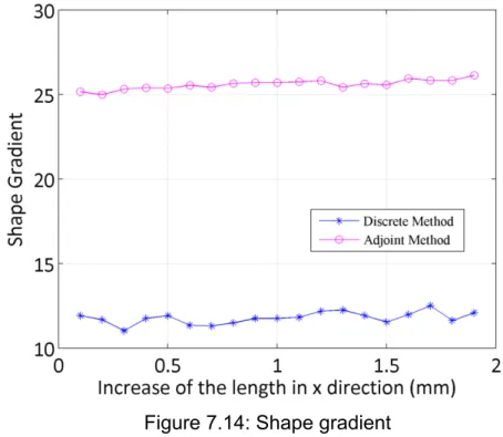
7.4.2 Thin 3D patch antenna enlarging along +x direction ... 79
7.4.3 Thick 3D antenna enlarging along +x direction ... 80
7.5 Shape gradient computation by different shape deformations ... 82
CHAPTER 8: NUMERICAL EXPERIMENTS ... 86
8.1 Antenna array location optimization using conjugate gradient and analytical gradient method ... 88
8.1.1 Illumination of single-frequency-single-incident wave ... 89
8.1.2 Illumination of multi-frequency-multi-incident wave ... 90
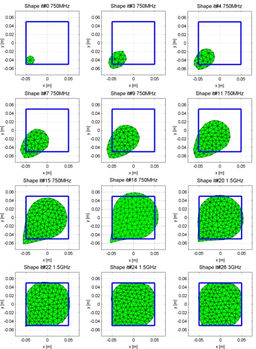
8.2 Shape Optimization of a single square patch antenna using nodal point mesh derivation ... 94
8.2.1 Shape Optimization from an initial guess in the center ... 94
8.2.2 Shape Optimization from an initial guess in the corner ... 97
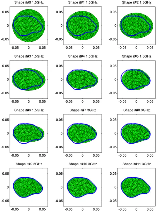
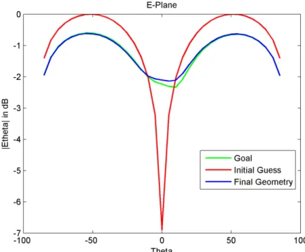
8.3 Shape optimization of a single patch antenna ... 101
8.3.1 Shape optimization using nodal point mesh derivation ... 102
8.3.2 Shape optimization using Topological Gradient without noise ... 104
8.3.3 Shape optimization using Topological Gradient with 20 dB noise ... 108
8.3.4 Shape Optimization using Topological Gradient with 10 dB noise ... 112
8.4 Shape Optimization of two rectangular patch antenna arrays using topological gradient ... 116
8.5 Shape Optimization of two circular patch antenna arrays ... 120
8.5.1 Shape Optimization using Frequency-hopping technique ... 121
8.5.2 Shape Optimization using multi-frequency technique ... 124
8.6 Shape Optimization of a single U-shape reflectarray element using topological gradient ... 130
8.6.1 Optimization from an initial guess of a larger size element ... 130
8.6.2 Optimization from an initial guess of a smaller size element ... 134
GENERAL CONCLUSION ... 143
Annex 1 - Spherical Coordinate System ... 146
Annex 3 - Signal-to-noise ratio for Robustness test ... 154
The inverse scattering problem for finding the optimal design of printed antenna arrays is particularly interesting for reflectarrays antennas and planar antenna arrays, which contain various types of printed elements. However, the design and optimization procedure require severe and efficient inverse and synthesis methods to meet the imposed constraints.
In this thesis, starting from Rumsey reaction concept, we describe an electromagnetic solver based on an integral formulation of the EM problem (SR3D code) for finding the forward electromagnetic solution. From this code, we have developed several inversion gradient-based algorithms to optimize planner antenna arrays. Especially, we give a new sense to the shape gradient versus an edge deformation (or transformation) in 3D for metallic layers with limited surfaces. The derived numerical model allows studying planar structures with the notion of metallic layer with a 2D outward normal direction.
In order to implement optimization procedure, we use level set method. The difficulty of the algorithm relies on finding the corresponding shape deformation velocities in the normal direction of contour, which we compute by the shape gradients (or shape sensitivity) versus radiation pattern modification taking into account the modeling of the antenna (Finite Element mesh).
In order to investigate the performance of the inverse algorithm and optimization procedure, different configurations are studied and shown in this thesis.
1.1 Antenna analysis and design
Antenna or antenna array structural design is a procedure to improve or enhance the performance of an existing structure by changing its parameters. The engineering design of the structural antenna in the simulation-based design process consists of antenna structure modeling, antenna design parameterization, antenna structure analysis, antenna geometry sensitivity analysis, and design optimization procedure.
The goal of antenna analysis is to determine the radiation characteristics, such as the radiation pattern and input impedance for a given antenna structure. The calculation of radiation pattern and input impedance requires solving Maxwell equations subject to certain boundary conditions, which are determined by antenna configurations. Unfortunately, we can only obtain analytical solution directly for a very few idealized and classical antenna geometries. However, for complex antenna structures, full-wave solutions to Maxwell equations are required to obtain reliable and accurate analysis.
Typically, the antenna design is based on numerical methods for solving Maxwell equations such as the Method of Moments (MoM), Finite Element Method (FEM), Finite Difference Time-Domain method (FDTD) and Transmission Line Matrix (TLM). Each numerical method has advantages and weak points concerning the computational cost, the level of accuracy, and the material modeling.
Antenna parametric studies are then performed to optimize the size of the structure under different constraints such as the return loss (S11 parameter), directivity, radiation pattern, polarization (linear, circular), or inter-element coupling. The quality of an optimized design is dependent on the parameterization of the optimization domain and the number of variables used. The use of a large number of variables leads to a large number of possible solutions and increases the complexity of the inverse problem.
1.2 Antenna optimization algorithms
Staring from an initial guess for the design variables of an existing geometry, optimization algorithms help to seek a solution of a formulated optimization problem by generating a sequence of updated design variables. In order to minimize the value of cost functional, at each step of optimization procedure, optimization algorithms are used to update the design variables by using the available information.
The multi-object optimization with the optimization of meta-heuristics (iterative stochastic algorithms) including evolutionary algorithms, such as the genetic algorithms (GA: Genetic Algorithms) [9-13], the simulated annealing (SA:
Simulated Annealing) algorithms, the particle swarm optimization (PSO: Particle Swarm Optimization) [14], ant colonies (ACO: Ant Colony Optimization) [15] or algorithms based on bad invasive weeds (IWO: invasive Weed Optimization) [16] or several hybrid stochastic algorithms [17], have been and are still widely used to optimize various electromagnetic devices. All evolutionary algorithms mentioned have shown their ability to find a global solution (in the sense of the global minimum of the objective or cost function to be minimized) of many optimization problems and synthesis of antennas and antenna arrays. However, the week number of parameters or information contained in the objective or cost function to minimize, combined with the random strategy of evolutionary algorithms, is ineffective and thus optimizes complex structures with a large number of variables.
Gradient-based optimization algorithms have been used to solve inverse scattering electromagnetic problems and antenna optimization. Gradient-based optimization algorithms can converge faster towards the minimum, but on the other hand, the global convergence cannot be guaranteed. However, we can still use some techniques, able to improve the convergence performance of gradient type optimization algorithms. Using a priori or extra information or fixing some constraints, to the optimization procedure or by modifying the cost functional using regularization for example, may enhance the global convergence. We can use extra information with a frequency hopping technique, where the optimization is performed with respect to several frequencies and defining the final cost functional combing the results derived from each frequency. We can also use a multi-frequency technique by gathering all the information derived from a sequence of frequencies at each iteration. In addition, we can also control the size of the optimal time step in when using level set method. A large time-step speeds up the inherently slow curve evolution process, but the question is: how large value of Δt can we use? It was observed that, for small values of the time-step, though the convergence was slow, curve evolution results were satisfactory. When large time-steps were used to speed up the evolution process, we often got garbage outputs. Clearly there is a stability issue that depends on the value of the time-step Δt employed. We can also use the value of the CFL (Courant-Friedrichs-Lewy) [29] coefficient. All these techniques are able to modify the convergence of the cost functional.
1.3 Topological Gradient and Level Set method
When solving a problem of topology optimization, the number of variables can easily reach to thousands or even millions for 2D and 3D cases. The optimization techniques of gradient type are generally preferred to solve problems with a large number of variables. The main reason is that the
gradient of the objective function or cost function contains a lot of important information. The shape gradient based on an adjoint formulation [1-8] is only valid for a 3D regular closed surface where the outward-pointing normal is defined everywhere, which is not the case for planar or patch antennas. The numerical models to study metal planar structures typically use the concept of perfect conducting layer in a plane domain bounded by a closed curve. Then in the case of open structures, or in the case of structures with edges, the definition of adjoint problem can be problematic or very complex mathematically. Therefore, it is particularly interesting to carry out sensitivity analysis from the objective or cost function to determine the most sensitive parameters to optimize. The precise calculation of the shape gradient for the miniaturization of antennas is an imperative one for topology optimization with gradient type methods.
Level Set method is extremely suitable for reflectarray antenna and planar antenna array optimization, since it is able to compute geometric quantities, and handle topology changes easily. The shape of elements can be merged and separated, because the Hamilton-Jacobi equation is working on a higher dimension, it means that it is not only able to optimize the shape of element, and also the element number.
2.1 General Questions
In general, for electromagnetic problems, there are two main problems to solve: the forward and inverse problem. For the forward problem, when the incident sources, geometry of the structures, and their electromagnetic properties are completely defined, we need to find the solution of their interaction. While for the electromagnetic inverse problem, when the interaction of the electromagnetic field is known in a certain domain, we need to determine the all properties of the illumined structures, including the geometry information, electromagnetic properties, provided the incident sources are known.
An important point for solving the electromagnetic inverse problem is that the inversion algorithm must be based on a solution of the forward modelling that correctly solves the electromagnetic responses or interaction.
In this work, we are going to use an electromagnetic solver named SR3D ("Structures Rayonnantes 3D" meaning "3D Radiating Structures") based on a method of moment, for solving the electromagnetic forward problem. In this chapter, starting from Maxwell equations, we introduce the theoretical basis of SR3D solver, with the reaction concept and the variational formulation.
2.2 Maxwell Equations
Maxwell equations describe the property of electromagnetic waves and fields. Consider a homogeneous, isotropic domain Ω with boundary Γ defined by electric permittivity ε, magnetic permeability µ and conductivity σ. The electromagnetic wave is described by E!"and H!"!, which corresponds to electric and magnetic fields, respectively. The Maxwell equations are defined here with a time-dependence e−i tω : ∇ × E!"= iω B!"− M! "! ∇ × H!"!= −iω D!"+ J!" ∇ ⋅ D!"=ρe ∇ ⋅ B!"=ρm % & ' ' ( ' ' (2.1) with:
ω angular frequency
J !"
electric current density M
! "!
magnetic current density D !" electric induction B !" magnetic induction
ρe electric charge density
ρm magnetic charge density
The Maxwell equations are first-order linear coupled differential equations relating the vector field quantities to each other. In addition to these four Maxwell equations, there are four medium-dependent equations, which are related with the constitutive relations:
m D E J E B H M H ε σ µ σ = = = = uv uv uv uv uv uuv uuv uuv (2.2) with: 0 0 r r ε ε ε µ µ µ = =
The magnetic and electric charge densities are defined as:
∇ ⋅ J!"− iωρe= 0 ∇ ⋅ M! "!− iωρm = 0
(2.3)
2.3 Boundary Conditions
The material medium in which EM field exists is usually characterized by its constitutive parameters: the electric permittivity ε, the magnetic permeability µ and the conductivity σ. Consider the situation in which one medium, characterized by ε1 and µ1 and σ1, shares an interface with another medium, characterized by ε2, µ2 and σ2. In order to solve for EM problems, at the interface, the tangential and normal fields must satisfy the boundary conditions:
n^× (H!"!2- H !"! 1) = J !" s n^× (E!"2- E !" 1) = −M ! "! s n^⋅ (D!"2- D !" 1) = ρes n^⋅ (B!"2- B !" 1) = ρms (2.4)
where n is a unit normal vector directed from medium 2 to medium 1. ^
Figure 2.1: Boundary Conditions
In the case of a PEC boundary, we can write them as:
n ^ × H!"!2= J !" s n^× E!"2 = −M ! "! s n ^ ⋅ E!"2 =ρes ε2 n ^ ⋅ H!"!2 = 0 (2.5) 2.4 Wave Equations
Maxwell equations are first-order coupled differential equations, difficult to solve as boundary-value problem. We can obtain a second-order differential equation (Helmholtz equation) that may be useful for solving electromagnetic problems.
We apply the operator
Δ
( )
= ∇∇⋅
( )
−∇×∇
( )
on the two first equations andobtain: Δ + k2
(
)
E!"= − i ωε ∇ !" ∇ !" ⋅ J!"+ k2!"J(
)
+ ∇ × M! "! Δ + k2(
)
H!"!= − i ωµ ∇ !" ∇ !" ⋅ M! "!+ k2M! "!(
)
− ∇ × J!" (2.6)with k wavenumber
k
=
ω εµ
The wave equation or Helmholtz equation can be written as:
Δ + k2
(
)
!"E= 0 Δ + k2(
)
!"!H= 0(2.7)
2.5 Surface Equivalence Theorem: Huygens Principle
To solve radiation and scattering problems, it is often useful to formulate the problem in terms of an equivalent one which may be more convenient to solve. In the analysis of electromagnetic problems, it is possible to replace the real sources defined in the investigation domain with superficial sources on a closed surface. According to the Huygens’ principle, we can substitute the general inhomogeneous volume problem with an ensemble of homogeneous and superficial problems, so that the problems of electric and magnetic fields can be replaced by the problems of surface currents, which can be defined as follows: J !" s= ˆn × H !"! s M ! "! s = − ˆn × E !" s ρes=ε ˆn ⋅ E!"s ρms =µ ˆn ⋅ H!"!s (2.8)
We can replace the problem (a) with problem (b) by using the superficial currents. In the special case (c), the material in V1 is an electric conductor, the
magnetic currents on the surface is zero, while in the case (d), the material in V1 is magnetic conductor, the electric currents on the surface is zero. [47]
Figure 2.2: Huygens’ equivalent Principle
2.6 Radiation Condition
The electromagnetic field must satisfy the next two conditions, which are the radiation conditions and finite energy conditions respectively:
lim n→∞ ˆn × ∇ !" × E!"− jk E!"
(
)
= o 1 r & ' ( ) * + lim n→∞ ˆn × ∇ !" × H!"!− jk H!"!(
)
= o 1 r & ' ( ) * + E !" 2 Ω∫
dΩ < ∞ H !"! 2 Ω∫
dΩ < ∞2.7 Green’s Function
The Green’s function is solution of the equation:
(
)
(
)
(
)
(
)
2 , , 1 if x=y=0 with: , 0 else k G x y x y x y δ δ Δ + = − ⎧ = ⎨ ⎩ (2.9)In ℜ!, we have the general solution:
(
,)
4 with: ikR e G x y R R xy π ± = = (2.10)The radiation condition shows that the scattered wave is only an outgoing wave. The Green’s function of the free space is then:
(
,)
( )
4 ikR e G x y G R R π = = (2.11)We can apply this equation to (2.6):
We then obtain: E !" r "
( )
= i ωε ∇ !" ∇!"⋅ +k2(
)
!"J#r"' $ % & ' (× G !" r " ,r"' # $ % & ' ( # $ % & ' ( − ∇ × M ! "! r "' # $ % & ' (× G !" r " ,r"' # $ % & ' ( # $ % & ' ( H !"! r "( )
= i ωµ ∇ !" ∇ !" ⋅ +k2(
)
M! "!#r"' $ % & ' (⋅G !" r " ,r"' # $ % & ' ( # $ % & ' ( + ∇ !" × J!"#r"' $ % & ' (× G !" r " ,r"' # $ % & ' ( # $ % & ' ( (2.12)2.8 EFIE and MFIE Equations Definition
If we apply the Huygens principle to the inhomogeneous radiation and scattering problems, we can thereafter describe this problem as an equivalent surface electromagnetic problem. It also means that scattering problems can be considered as radiation problems where the local radiating currents are generated by other currents or fields.
We can firstly write the total field as:
E !" r "
( )
= E!"inc( )
r" + E!"sca( )
r" H !"! r "( )
= H!"!inc( )
r" + H!"!sca( )
r" (2.13)Using the Green’s function, we can integrate over a closed surface domain Γ , where we have equivalent surface currents. Then, we can obtain the scattered field, and the total field:
E !" r "
( )
= E!"inc( )
"r + jωµ G Γ#∫
r",r!"'( )
J!" r!"'( )
dΓ + j ωε ∇ !" r' !" G Γ#∫
r",r!"'( )
∇!"Γ⋅ J !" r' !"( )
dΓ − ∇!"× G Γ#∫
r",r!"'( )
M! "! r!"'( )
dΓ (2.14) H !"! r "( )
= H!"!inc( )
r" + jωε G Γ#∫
r",r!"'( )
M! "! r!"'( )
dΓ + j ωµ ∇ !" r' !" G Γ#∫
r",r!"'( )
∇!"Γ⋅ M ! "! r!"'( )
dΓ − ∇!"× G Γ#∫
r",r!"'( )
!"J r!"'( )
dΓ (2.15)The unknown local currents J and M are created by an external but known incident field E!"inc and H!"!inc, the field E and H can be solved by an integral equation. E !"inc r "
( )
= jωµ G Γ#∫
r",r!"'( )
J!"a r' !"( )
dΓ + j ωε ∇ !" r' !" G Γ#∫
r",r!"'( )
∇!"Γ⋅ J !" a r' !"( )
dΓ − ∇!"× G Γ#∫
r",r!"'( )
M! "!a r' !"( )
dΓ (2.16) H !"!inc r "( )
= jωε G Γ#∫
r",r!"'( )
M! "!a r' !"( )
dΓ + j ωµ ∇ !" r' !" G Γ#∫
r",r!"'( )
∇!"Γ⋅ M ! "! a r' !"( )
dΓ − ∇!"× G Γ#∫
r",r!"'( )
J!"a r' !"( )
dΓ (2.17)We have to enforce the boundary conditions on the tangential electric and magnetic fields: n^(r) × E!"sca
( )
r" = −n^(r) × E!"inc( )
r" n ^ (r) × H!"!sca( )
"r + n ^ (r) × H!"!inc( )
r" = J!"( )
r" (2.18)This allows us to write the above in terms of the known incident electric field
E
!"inc
r
!
( )
and magnetic field !"!Hinc( )
r! as:ˆn × E!"inc
( )
r" = − ˆn × jωµ G Γ#∫
r",r!"'( )
!"J r!"'( )
dΓ % & ' + j ωε ∇ !" r' !" G Γ#∫
r",r!"'( )
∇!"Γ⋅ J !" r!"'( )
dΓ − M! "! r!"'( )
Γ#∫
∇!"r' !" G r",r!"'( )
dΓ−1 2 ˆn × M ! "! r!"'( )
*+ , (2.19) ˆn × H!"!inc( )
r" = − ˆn × jωε G Γ#∫
r",r!"'( )
M! "! r!"'( )
dΓ % & ' + j ωε ∇ !" r' !" G Γ#∫
r",r!"'( )
∇!"Γ⋅ M ! "! r!"'( )
dΓ + J!" r!"'( )
Γ#∫
× ∇!"r' !" G r",r!"'( )
dΓ +1 2 ˆn × J !" r' !"( )
*+ , (2.20)These two equations are called as the Electric Field Equation (EFIE) and the Magnetic Field Equation (MFIE).
2.9 Reaction Concept
The variational formulation can be obtained using the Rumsey reaction concept. Given an homogeneous domain Ω, with boundary surface Γ, sources
J
!" ,M! "!
{
}
and test sources{
J!"test,M! "!test}
defined along the tangent direction of surface Γ and with boundary condition defined, then the reaction of sources on the test sources in Ω is defined as a following bilinear form:RΩ"
{
!"J,M! "!}
, J{
!"test,M! "!test}
# $ % & ' = E !" ⋅ J!"test− M"! "!test⋅ H!"! # $ % & ' " # $ % & ' Γ#∫
dΓtest (2.21)Where the electromagnetic field
{
E!", H!"!}
is generated by the surface currentsJ
!" ,M! "!
{
}
defined inside Ω. We can also apply this concept to the incident electromagnetic field{
E!"inc, H!"!inc}
generated by the surface currents !"Ja, M! "!
a
{
}
RΩ J!"a,M ! "! a
{
}
, J{
!"test,M! "!test}
" # $ % & ' = E !"inc⋅ J!"test− M"! "!test⋅ H!"!inc # $ % & ' " # $ % & ' Γ
#∫
dΓtest (2.22)Both bilinear forms (C2.20) and (C2.21) have a symmetric property. So we can write the reciprocity principle:
RΩ"
{
!"J,M! "!}
, J{
!"test,M! "!test}
# $ % & ' = RΩ J !" a,M ! "! a{
}
, J{
!"test,M! "!test}
" # $ % & ' (2.23) 2.10 Variational FormulationIf we use the equation (C2.16) and equations shown in (C2.20) and (C2.21), and apply the boundary conditions, we obtain:
RΩ"
{
!"J,M! "!}
, J{
!"test,M! "!test}
# $ % & ' − RΩ J !" a,M ! "! a{
}
, J{
!"test,M! "!test}
" # $ % & ' = 0 (2.24)We also defineE!"= jωµ0e", M! "!= jωµ0!"pand!"J = j", develop equation (C2.20).
After few mathematical transformations, we can obtain:
−S E"!"inc, H!"!inc, j"test, p!"test # $ % & ' = µR1 j " , j"test " # $ % & ' +k 2 µr R1"!"p, p!"test # $ % & ' + R2""j, p!"test # $ % & ' + R2 p !" , j"test " # $ % & ' (2.25)
The kernel terms can be defined as follows:
R1!a!,a!test " # $ % & =
( )
G a ! ⋅ a!test ! " # $ % &"∫
"∫
dΓdΓtest − 1 k2( )
G ∇ #! ⋅ a!∇#!⋅ a!test ! " # $ % &"∫
"∫
dΓdΓtest R2!a!,b!test " # $ % & = ∇ r !' # !## G × a!(
)
⋅ b!test ! " # $ % &"∫
"∫
dΓdΓtest (2.26)If we apply the Huygens principle for a homogenous domain Ω, the domain can be divided in several sub-domains Ωi , by considering the boundaries Γi generated by the subdomains Ωi,. Therefore, we can define the Rumsey concept on different Nd subdomains:
RΩ i J !" ,M! "!
{
}
, J!"i test ,M! "!i test{
}
" # $ % & ' − RΩi J !" a,M ! "! a{
}
, J!"i test ,M! "!i test{
}
" # $ % & ' i=1 Nd∑
= 0 (2.27)− S E"!"inc, H!"!inc, j"test, p!"test # $ % & ' i=1 Nd
∑
= µR1i j " , j"test " # $ % & ' +k 2 µr R1i p !" , p!"test " # $ % & ' ) * + i=1 Nd∑
+R2i""j, p!"test # $ % & ' + R2i p !" , j"test " # $ % & ', -. (2.28) .28)In this chapter, we start from the Rumsey reaction equation written in chapter 2, then define the MoM linear system, and finally describe every term of the linear system, including the reaction matrix and source vector.
3.1 Linear System
We can write the Rumsey reaction form related to a single couple of triangles TK and TL: −S E"!"inc, H!"!inc, j"K, p!"K # $ % & ' =µR1KL"!jL, j!K # $ % & ' +k 2 µr R1 KL"!"pL, p!"K # $ % & ' + R2KL""jL, p!"K # $ % & ' + R2 KL"!"pL, j"K # $ % & ' (3.1)
Figure 3.1: Coupling reaction between triangles
The terms R and S, which denote the coupling terms and source vector respectively, are defined by the following equation:
R1!a!L,a!K " # $ % & = G x ! , y"!
( )
!a!L( )
"!y ⋅ a!K( )
x! " # $ % & TL!∫
T!∫
K dydx −4HKHL k2 G x " , y#"( )
TL!∫
T!∫
K dydx R2!a"L,b"K " # $ % & = ∇#"#"yG x " , y#"( )
× a!L( )
"!y ! " # $ % &⋅ b !K x !( )
TL!∫
T!∫
K dydx S E!"#inc, H"#"inc, j#K, p"#K " # $ % & = E "#inc ⋅ j#K− H"#"inc⋅ p"#K ! " # $ % &dx T∫
K (3.2)1
where: , is the surface of triangle T
2
T T
T
H = Λ
Λ
Then we can define the sub-linear system related to the triangles TK and TL
as:
K KL L
S Z
⎡ ⎤ =⎡ ⎤ ⎡Φ ⎤
⎣ ⎦ ⎣ ⎦ ⎣ ⎦ (3.3)
The electric JL and magnetic ML density surface currents contained in ΦL are the solutions of the sub-system. The numerical modeling of the antennas is based on surface discretization, using triangular finite element cells. The matrix ZKL depends on the structure geometry of the ensemble of triangles TK and TL of the mesh, in which the different triangles summits are CiK and CiL (i=1,2,3). S is the second member, associated with the incident fields.
If we consider the global antenna structure, which contains all the discretized triangles, by considering all the coupling reactions and the second member, the whole linear system of MoM, can be finally defined as follow:
[ ] [ ][ ]
S
=
Z
Φ
(3.4)Then we can write the whole linear system as below:
S1 ! Sn−1 Sn " # $ $ $ $ $ % & ' ' ' ' ' = Z1,1 " Z1,n−1 Z1,n ! # ! ! Zn−1,1 " Zn−1,n−1 Zn−1,n Zn,1 " Zn,n Zn,n " # $ $ $ $ $ $ % & ' ' ' ' ' ' J1 ! Jn−1 Jn " # $ $ $ $ $ % & ' ' ' ' ' (3.5)
[ ]
Z
is an n*n symmetrical matrix, where n is the number of degrees of freedom of the antenna structure. For each degree of freedom, we compute the coupling reaction between others and itself, and the second member.3.2 Reaction Matrix Z
If we consider the sub-linear system related to triangles TK and TL as written
in equation (3.3), the combination of matrix elements ZKL
⎡ ⎤
⎣ ⎦ is a 6*6
TK and TL respectively. The elements of ⎡⎣ZKL⎤⎦ are placed at different location
within the global matrix, as the matrix element is ranged according to the
arrangement of fluxes. The sub-matrix KL
ee
Z
⎡ ⎤
⎣ ⎦ denotes the coupling reaction
given by electric-electric currents, KL em Z ⎡ ⎤ ⎣ ⎦ by electric-magnetic currents, KL me Z ⎡ ⎤ ⎣ ⎦
by magnetic- electric currents, and KL
mm Z ⎡ ⎤ ⎣ ⎦ by magnetic-magnetic currents. We hav KL KL ee C S em C S KL C S KL KL me C S mm C S Z Z Z Z Z × × × × × ⎡⎡⎣ ⎤⎦ ⎡⎣ ⎤⎦ ⎤ ⎢ ⎥ ⎡ ⎤ = ⎣ ⎦ ⎢⎡ ⎤ ⎡ ⎤ ⎥ ⎣ ⎦ ⎣ ⎦ ⎣ ⎦ (3.6)
where C denotes the number of Cartesian coordinates, S the number of triangle vertices, e is the electric reaction, m the magnetic reaction. In our system, C and S are equal to 3.
Figure 3.2: Coupling reaction between triangles K and L
We first define all the geometric variables related to triangles TK and TL in
equation (3.7). In Figure 3.2, we describe the geometric relationship between triangles TK and TL, and x and y are the points defined in the triangle TK and TL respectively.
r ! = y − x
(
" !"""")
, r = y − x! "!!!! x", y!"∈ TK,TL ∈ ℜ3 x " = x$% 1, x2, x3&', y!"= y$% 1, y2, y3&' C!"s T = CcsT = C$% 1sT,C2sT,C3sT&' ∈ ℜ3, c,s = 1,2,3where: c is the Cartesian coordinate index
s is the vertex index number
(3.7)
Then, we define the matrix by terms of electric and magnetic properties as follows: 2 cs cs cs cs KL KL ee C S ee C S se KL KL em C S em C S se KL KL me C S me C S sm KL KL mm C S mm C S sm Z R I Z R I Z R I k Z R I µ µ × × × × × × × × ⎡ ⎤ = ⎡ ⎤ ⎣ ⎦ ⎣ ⎦ ⎡ ⎤ =⎡ ⎤ ⎣ ⎦ ⎣ ⎦ ⎡ ⎤ =⎡ ⎤ ⎣ ⎦ ⎣ ⎦ ⎡ ⎤ = ⎡ ⎤ ⎣ ⎦ ⎣ ⎦ (3.8)
where µ denotes the magnetic permeability, k the wavenumber of the electromagnetic radiation and I terms is the coupling terms (-1 or +1), related to the degrees of freedom, needed to represent the global reaction matrix. Thereby, using this reference we can explicit these terms as follows:
R1aaKL
→ ReeKL, RmmKL
represented by the same kind of electric or magnetic currents, ee or mm
R2abKL
→ RemKL, RmeKL
represented by the different kind of electric or magnetic currents, em or me
(3.9)
For sake of completeness, we can define the A, D, T, F operator expressions:
AKL G
( )
= G x( )
!, y"! !a!L( )
"!y ⋅ a!K( )
x! " # $ % & TL#∫
dy dx T#∫
K DKL G( )
= HKHL G x ! , y"!( )
TL#∫
dy dx T#∫
K TKL G( )
= ∇"!y"!G x ! , y"!( )
× a!L( )
"!y ! " # $ % &⋅ b! K x !( )
TL#∫
dy dx T#∫
K where: G = e jkr r , r = y − x " !"""" (3.10)We can define the extended form of basis function with α!" and β!" for the triangle TK and TL: ΘK
( )
x! ! "# $%&=α !"K =β!"K = H! K( )
C! "!!3x HK( )
C! "!!1x HK( )
C! "!!2x "# $ %& ΘL( )
!"y ! "# $%&=α !"L =β!"L= H! L( )
C! "!!3y HL( )
C! "!!1y HL( )
C! "!!2y "# $ %& ΔKL( )
x!, y"! ! "# $%&= ∇ !" y !"G x", y!"( )
× a!L( )
"!y ! " # $ % &⋅ b !K x !( )
! " # $ % & where: HT = 12ΛT , ΛT is the surface of triangle T
(3.11) If we suppose: ΘK
( )
x! ! "# $%&= HK C3x ! "!!( )
( )
C! "!!1x( )
C! "!!2x ! "# $ %&= HK B K x!( )
! "# $%& ΘL( )
!"y ! "# $%&= HL C3y ! "!!( )
( )
C! "!!1y( )
C! "!!2y ! "# $ %&= HL B L !"y( )
! "# $%& where: BK x!( )
= C!( )
! "!!3x( )
C! "!!1x( )
C! "!!2x "# $ %& BL y !"( )
= C3y ! "!!( )
( )
C! "!!1y( )
C! "!!2y ! "# $ %& φ( )
r = G r( )
=e jkr r ψ( )
r =∂φ( )
r ∂r = jkr −1(
)
ejkr r3 ∇!"G r( )
= ∇!"φ( )
r =ψ( )
r ⋅ r (3.12) 2) We obtain:ΔKL
( )
x!, y!" " #$ %&'cs=ψ r( )
⋅ r ! × HL"BL( )
!"y #$ %&'s⋅ HK BK x!( )
" #$ %&'c = ψ r( )
HK BK x!( )
" #$ %&'c× HL BL !"y( )
" #$ %&'s{
}
⋅ r ! =HKHLψ r( )
"ΩKL( )
x!, y!" #$ %&'cs ΩKL( )
x!, y!" "#$ %&'cs= det cols
BL !"y
( )
" #$ %&'| colc B K x!( )
" #$ %&'| y − x ! "!!!! " # %&(
)
where: BT w!"( )
" #$ %&'i = coli B T w!"( )
" #$ %&' (3.13)We can define a simpler formula for A, D, T operators as follows:
( )
( )
( )
( )
( )
( )
( )
( )
( )
, , , , , 1,2,3where: Cartesian coordinates index s = triangle v K L K L K L KL K L K L cs c s T T KL K L cs T T KL KL K L cs cs T T A H H x y B x B y dydx D H H x y dydx T H H x y x y dydx c s c φ φ φ φ ψ ψ ⎡ ⎤ ⎡ ⎤ ⎡ ⎤ = ⎣ ⎦ ⎣ ⎦ ⎣ ⎦ ⎡ ⎤ = ⎣ ⎦ ⎡ ⎤ ⎡ ⎤ = Ω ⎣ ⎦ ⎣ ⎦ = =
∫ ∫
∫ ∫
∫ ∫
v uv v uv v uv v uv v uv——
——
——
ertex index (3.14)Until now, we have defined the kernel of the coupling reactions between two triangles TK and TL, we can express the formulas using the operators A, D, T:
( )
( )
( )
(
)
{
}
( )
( )
( )
( )
2 2 2 2 4 4 4 cs cs cs cs KL KL KL ee C S cs cs se KL KL se cs cs KL KL em C S cs se KL KL me C S cs sm KL KL KL mm C S cs cs s Z A D I k A D k I Z T I Z T I k Z A D I k µ φ φ µ φ φ ψ ψ φ φ µ × − × × × ⎧ ⎫ ⎡ ⎤ = ⎨⎡ ⎤ − ⎡ ⎤ ⎬ ⎣ ⎦ ⎩⎣ ⎦ ⎣ ⎦ ⎭ ⎡ ⎤ ⎡ ⎤ = ⎣ ⎦ +⎣ − ⎦ ⎡ ⎤ =⎡ ⎤ ⎣ ⎦ ⎣ ⎦ ⎡ ⎤ =⎡ ⎤ ⎣ ⎦ ⎣ ⎦ ⎧ ⎫ ⎡ ⎤ = ⎨⎡ ⎤ − ⎡ ⎤ ⎬ ⎣ ⎦ ⎩⎣ ⎦ ⎣ ⎦ ⎭(
)
( )
{
2}
1 4 cs cs m KL KL sm cs cs A k φ D φ I µ ⎡ ⎤ ⎡ ⎤ = ⎣ ⎦ − ⎣ ⎦ (3.15)(
)
3 2 2 , = 1 , 4 , = jkr jkr jkr jkr e e jkr r r e e k r r k φ ψ χ = − Γ = − (3.16)We finally obtain the discrete expressions for the KL
xx Z ⎡ ⎤ ⎣ ⎦
( )
( )
{
}
( )
( )
( )
( )
{
}
1 4 cs cs cs cs KL KL KL ee C S cs cs se KL KL em C S cs se KL KL me C S cs sm KL KL KL mm C S cs cs sm Z A D I Z T I Z T I Z A D I µ φ ψ ψ χ φ µ × × × × ⎡ ⎤ = ⎡ ⎤ +⎡ Γ ⎤ ⎣ ⎦ ⎣ ⎦ ⎣ ⎦ ⎡ ⎤ = ⎡ ⎤ ⎣ ⎦ ⎣ ⎦ ⎡ ⎤ = ⎡ ⎤ ⎣ ⎦ ⎣ ⎦ ⎡ ⎤ = ⎡ ⎤ − ⎡ ⎤ ⎣ ⎦ ⎣ ⎦ ⎣ ⎦ (3.17)3.3 Source Vector Definition
We first define an electric dipole as a source for the scattering computation. The source vector of the linear system takes into account the sources defined inside the analysis domain. The reaction between the source and the discrete triangle (metallic or dielectric) is considered. We then obtain a vector SK.
Figure 3.3: Source Vector
Source vector Dipole: The source vector is considered as the reaction between an incident dipole DK in free space and a single triangle TK of a
metallic or dielectric mesh of a discretized structure. We can write the coupling reaction vector as:
2 1 2 1 2 1 K e C K C K m C
S
S
S
× × ×⎡
⎡
⎣
⎤
⎦
⎤
⎢
⎥
⎡
⎤
=
⎣
⎦
⎢
⎡
⎤
⎥
⎣
⎦
⎣
⎦
(3.18) where:C = 3, number of the cartesian coordinates K = triangle index
e = electric reaction m = magnetic reaction
Suppose we have N discrete triangles in the whole domain, the source vector S should have 6*N rows in total. It can be represented as:
S ! " #$ = S1 ! " #$6 ! SK ! " #$6 ! SN ! " #$6 ! " % % % % % % % % # $ & & & & & & & & (3.19)
We define all the geometry variables for triangle TK and dipole DK:
r ! = x − y
(
!!!!!!D")
, r = x − y!!!!!!D" x"∈ TK ∈ ℜ3, y!"D ∈ TK ∈ ℜ3 x ! = x!" 1, x2, x3#$, y!"D= y!" 1D, y2D, y3D#$ C!"s K = CcsK = C!" 1sK,C2sK,C3sK#$ ∈ ℜ3, c,s = 1,2,3where: c is the Cartesian coordinate index
s is the vertex index number
(3.20)
The terms of vector SK can be defined as follows:
SeK!m!"D, y!"D " # $ % & ' ( ) * + , c = −µ φ x!!, y!"D " # $ % & TK
!∫
'()ΘK( )
x! *+, cm !" t D x ! , y!"D ! " # $ % & 0 1 2 + 1 k x − y!!!!!!D" j − 1 k x − y!!!!!!D" ! " # # # $ % & & & 2 Θ K x!( )
' () *+,cm !"D ! " # −3 ΘK x!( )
' () *+,cm !" t D x ! , y!"D ! " # $ % &$ % &34 5dx SmK!m!"D, y!"D " # $ % & ' ( ) * + , c = −µ ψ x!!, y!"D " # $ % & εK x ! , y!"D ! " # $ % & ' ( ) * + , c dx TK!∫
(3.21)where: εK!x!, y"!D " # $ % & ' ( ) *+, c
= det col! c!"#ΘL
( )
"!y $%&m"!D r! " # $ % & m"!D= m"!1 D ,m"!2 D ,m"!3 D ! "# $%&, dipole D with dipole moment m "!D m"!t D x ! , y"!D ! " # $ % & = m "!D − m"!D⋅ r ! r ! " # # $ % & &⋅ r ! r ! " # # $ % & & ' ( ) ) * + ,
,, dipole D transversal dipolar moment m "!
t D
We can reduce the term K
ε
as: εK!x!, y"!D " # $ % & ' ( ) * + , c= det col! c!"#ΘL
( )
!"y $%&m!"D r" " # $ % & = HK ϒ K!x!, y"!D " # $ % & ' ( ) * + , c (3.22) with: ϒK"x!, y"!D # $ % & ' ( ) * + , -c = det colc B K x!( )
( )* +,-m !"D r " " # $ % & 'The reduced form of the source vector can be written as:
SeK!m!"D, y!"D " # $ % & ' ( ) * + , c = −µHK φ x!!, y!"D " # $ % & T
!∫
K BK x!( )
' () *+,c m !" t D x ! , y!"D ! " # $ % & / 0 1 + 1 k x − y!!!!!!D" j − 1 k x − y!!!!!!D" ! " # # # $ % & & & 2 BK x!( )
' () *+,c m !"D ! " # −3 BK x!( )
' () *+,c m !" t D x ! , y!"D ! " # $ % &$ % &23 4dx SmK!m!"D, y!"D " # $ % & ' ( ) * + , c = −µHK ψ x!!, y!"D " # $ % & ϒK x ! , y!"D ! " # $ % & ' ( ) * + , c dx T!∫
K (3.23)3.4 Reaction Matrix Discretization
From a computational point of view, we need to discretize A, D, T operators, and
⎡
⎣
Z
xxKL⎤
⎦
term. We use a seven-point Gauss discretization method to discretize all the terms.We define the normalized Gauss method weights γT for a genetic
2
where: is non-normalized Gauss weight for the w point
w w w T T w H α γ α α = Λ = (3.24)
Figure 3.4: Reaction Matrix discretization
In figure 3.4, we apply a seven-Gauss method to the triangle TK and TL. Thereafter, we can write the discretized form of a generic Green’s function kernel as: G !x, !y
( )
= γKγLG !x(
K, !yL)
L∑
K∑
= 1 4HKHL γKγLG !x(
K, !yL)
L∑
K∑
(3.25)According to the equation (3.14), the A, D, T operators and
⎡
⎣
Z
xxKL⎤
⎦
terms can be discretized as follows:AKL g 1
( )
! " #$cs= HKHL 1 4HKHL αkαlg1 x ! k, y !" l(
)
BK x! k( )
! "# $%& l∑
c t k∑
BL !"y l( )
! "# $%&s DKL g 2( )
! " #$cs= HKHL 1 4HKHL αkαlg2 x ! k, y !" l(
)
l∑
k∑
TKL g 3( )
! " #$cs= HKHL 1 4HKHL αkαlg3 x ! k, y !" l(
)
l∑
k∑
ΩKL x!k, y !" l(
)
! "# $%&cs where: g1 x!k, y !" l(
)
= φ x!k, y !" l(
)
χ x!k, y !" l(
)
! " # $ # , along with g2 x!k, y !" l(
)
= Γ x!k, y !" l(
)
φ x!k, y !" l(
)
! " # $ # g3 x!k, y !" l(
)
= Ψ x!k, y !" l(
)
{
(3.26)The reduced form can be written as:
AKL g 1
( )
! " #$cs= 1 4 αkαlg1 x ! k, y "! l(
)
BK x! k( )
! "# $%& l∑
c t k∑
BL !"y l( )
! "# $%&s DKL g 2( )
! " #$cs= 1 4 αkαlg2 x ! k, y "! l(
)
l∑
k∑
TKL g 3( )
! " #$cs= 1 4 αkαlg3 x ! k, y "! l(
)
l∑
k∑
ΩKL x!k, y "! l(
)
! "# $%&cs (3.27)The discretized form for the term ⎡⎣ZxxKL⎤⎦ can be written as:
( )
( )
{
}
( )
( )
( )
( )
{
}
1 4 cs cs cs cs KL KL KL ee CS cs cs se KL KL em CS cs se KL KL me CS cs sm KL KL KL mm CS cs cs sm Z A D I Z T I Z T I Z A D I µ φ ψ ψ χ φ µ ⎡ ⎤ = ⎡ ⎤ +⎡ Γ ⎤ ⎣ ⎦ ⎣ ⎦ ⎣ ⎦ ⎡ ⎤ =⎡ ⎤ ⎣ ⎦ ⎣ ⎦ ⎡ ⎤ =⎡ ⎤ ⎣ ⎦ ⎣ ⎦ ⎡ ⎤ = ⎡ ⎤ − ⎡ ⎤ ⎣ ⎦ ⎣ ⎦ ⎣ ⎦ (3.28))3.5 Source Vector Discretization
For the source vector, in order to implement numerical computation, we need also to discretize the source vector. The method of discretization is based on the same seven-point Gauss discretization method. (Shown in Figure 3.5)
Figure 3.5: Source vector discretization
By applying the discretization method, we can obtain the reduced form for the source vector terms:
SeK!m!"D, y!"D " # $ % & ' ( ) * + , c = −µ 2 αkg1 x ! k, y "!D ! " # $ % & BK x ! k
( )
! "# $%&c m !" t D x " k, y !"D ! " # $ % & ' ( ) k∑
+ 1 k xk− yD !!!!!!!" j − 1 k xk− yD !!!!!!!" ! " # # # $ % & & & 2 BK x! k( )
! "# $%&c m !"D ! " # −3 BK x! k( )
! "# $%&c m !" t D x " k, y !"D ! " # $ % &'( ) SmK!m!"D, y!"D " # $ % & ' ( ) * + , c = −µ 2 αkg3 x ! k, y "!D ! " # $ % & ϒK x ! k, y "!D ! " # $ % & ' ( ) * + , k∑
c where: g1 x!k, y "!D ! " # $ % & = φ x ! k, y "!D ! " # $ % & g3 x!k, y "!D ! " # $ % & = φ x ! k, y "!D ! " # $ % & (3.29)Global and local optimization algorithms are broadly divided into deterministic and stochastic. In this chapter, starting from the concept of global and local optimization, we introduce several deterministic and stochastic optimization methods, and discuss the advantages and weak points of each one.
4.1 Global and Local Optimization
Normally, most of optimization techniques focus on search and optimization problems associated with minimizing a cost functionF F=
( )
Ω . We can define the solution set for an optimization problem:( )
{
( )
( )
}
argmin : for all
x X
X∗ F x x∗ X F x∗ F x x X
∈
= = ∈ ≤ ∈ (4.1)
Where x is a p-dimensional vector of parameters that being adjusted and X ⊆ ° pis the domain for x, which represents constraints on allowable values for x. The statement
( )
arg minx X∈ F x
illustrates that X∗ is the set of values x x∗
= (x the “argument” in “arg min”)
that minimizesF x
( )
subject to x∗ satisfying the constraints represented in the setX . [49]Figure 4.1 illustrates a simple distinction of local and global minima for a one-dimensional optimization problem. When the optimal value equals to
x
local, the value of cost function isF x(
local)
, however, it is not the lowest of cost function from the global viewpoint, comparing with a global optimal pointx∗, where the value of cost function isF x( )
∗ .Figure 4.1: Local and global minima
The difference between global and local optimization is one of the major distinction in optimization techniques. When considering all other factors in the optimization problems equally, one would always hope to find a globally optimal solution, which can provide a lowest value of cost function, and normally a better similarity comparing with the goal. While in practice, especially for nonlinear problems, the cost function always has a large number of local minima. Finding an arbitrary local optimum is relatively straightforward by using classical local optimization methods, and finding the global minimum of a function is far more difficult. In this situation, a global solution may not be always available and sometimes a local minimum is better than any in its vicinity, but can be an acceptable result.
When we consider the concept of local optimization, it means that the optimization procedure attempts to find a local minimum, and obtaining the global minimum cannot be guaranteed. Local optimization algorithms generally depend on derivatives of the cost function and constraints to aid in the search procedure. Thus, there are strict requirements for the input information.
4.2 Stochastic Method
Stochastic methods normally can locate a global optimum faster than deterministic ones and only offer a guarantee in probability. In additional, stochastic methods can adapt better to unknown formulations and extremely ill-behaved functions, whereas deterministic methods usually rely on some analytical assumptions about the problem formulation and its analytical properties. However, in general search and optimization, it is very difficult to develop automated methods for indicating when the algorithm is close enough to the solution that it can be stopped, and it cost a considerable computation
for finding optimal solutions. We introduce some popular stochastic methods below.
4.2.1 Genetic Algorithms
The genetic algorithm was first introduced by Holland (1975) [52], and has become a popular method for solving large optimization problems with multiple local optima. In a genetic algorithm, a population of candidate solutions to an optimization problem is evolved toward better generations. Each candidate solution has a set of properties, which are represented in binary, and considered as 0s and 1s. The evolution usually starts from a population of randomly generated individuals, and then for each generation or iteration, the fitness of every individual in the population is evaluated stochastically by selecting the multiple individuals from the current population. When a solution is found that satisfies minimum criteria for the population, the algorithm terminates and we can obtain optimal solution.
However, in order to find the optimal solution for complex high-dimensional and multimodal problems, very expensive cost function evaluations are often required. When we solve the practical problems such as structural optimization problems, typical optimization methods may not be able to deal with it. Moreover, a genetic algorithm needs a considerable number of computations and iterations before finding the convergence towards the optimum.
4.2.2 Particle Swarm Optimization
Particle swarm optimization (PSO) is a population based stochastic optimization technique developed by Eberhart and Kennedy in 1995 [53]. It is a computational method that optimizes a problem by iteratively trying to improve a candidate solution with regards to a given measure of quality.
PSO shares many similarities with evolutionary computation techniques such as Genetic Algorithms. The optimization system is randomly initialized with a population of solutions and searches for optima by updating generations. PSO optimizes a problem by moving the potential solutions, which are called the particles, around in the search-space according to simple mathematical formulae over the particle's position and velocity.
PSO is a metaheuristic method, which makes few or no assumption about the problem being optimized and can search very large spaces of candidate solutions. However, it cannot guarantee an optimal solution is ever found, and is easily trapped into a local minimum.