Artifact Detection in Physiological
Parameter Trend Data
By
Kuo-Hsiung Hanson Wong
Submitted to the Department of Electrical Engineering and Computer Science in Partial Fulfillment of the Requirements for the Degree of Master of Engineering in Electrical Engineering and Computer Science
at the Massachusetts Institute of Technology February 10, 2003
Copyright 2003 MIT. All rights reserved.
MASSACHUSETTS INSTITUTE OF TECHNOLOGY
JUL
3 0 2003
LIBRARIES Authord5epartment
of Electrical Engineering and Computer Science February 10, 2003 Certified by Roger G. Mark Thesis Supervisor Accepted by A e Arthur C. Smith Chairman, Department Committee on Graduate ThesisArtifact Detection in Physiological
Parameter Trend Data
By
Kuo-Hsiung Hanson Wong
Submitted to the Department of Electrical Engineering and Computer Science February 10, 2003
In Partial Fulfillment of the Requirements for the Degree of Master of Engineering in Electrical Engineering and Computer Science
Abstract
Physiological signals recorded in an intensive care unit are often corrupted by artifactual data. This results not only in false alarms but also in problems analyzing the data in a research environment. This project presents an alternative method for artifact detection using both higher-level limits on single-signal variation as well as correlations between multiple related signals. Analysis of the algorithm was performed using parameter trend data from 34 ICU patients. Problems with this specific data set resulted in lower values for sensitivity and positive predictivity. Overall, the sensitivity and positive predictivity for the algorithm are 78% and 66%, respectively.
Thesis Supervisor: Roger G. Mark, M.D., Ph.D.
Distinguished Professor in Health Sciences and Technology, HST Professor of Electrical Engineering and Bioengineering,
Department of Electrical Engineering and Computer Science, MIT Chapter 1 - Introduction
1.1 ICU
Patients in an intensive care unit (ICU) are monitored using devices that measure and record a large number of physiological signals with the purpose of obtaining a comprehensive view of their physiological state at a particular time. These devices usually incorporate simple alarm functions that are meant to alert the ICU staff to the arrival of an "event," a change in the signal property that is associated with an underlying pathophysiological process. Such alarms make use of threshold detection and sound when a signal value exceeds a certain threshold. Signals of interest often include heart rate, blood pressure, and other variables but differ depending upon the patient and his or her condition.
Comparisons with predetermined thresholds are done on each signal separately with no inter-signal relationship taken into account. Problems arise, in part, from this lack of coupling. Certain physiological signals are correlated with each other, as is the case with heart rate and mean arterial blood pressure. However, if one single-signal alarm is triggered, other signals are not examined to see if similar events are detected
among them. A result of this process is a prevalence of false alarms.
An alarm goes off every 30 seconds in a typical full ICU.' Studies have shown that a high percentage of these alarms are incorrect. Zong found that 35% of alarms in a collection of ICU recordings were false while Tsien found that up to 80-90% of all
alarms could be classified as not meaningful. Though a small percentage (6%) of alarms in Tsien's study were clinically irrelevant true alarms, the remaining were
false-2,3
placed on patients and their families but also a reduction in the trust placed on the machines by the ICU staff.
Artifacts - significant changes in the values of the signal not due to physiological changes in the patients - are common in ICU data recordings and are the predominant cause of false alarms. Such artifacts may also result in delayed warnings or, in the worst
case, prevent the identification of important events altogether. Unfortunately, there are many causes of artifacts. Interference, unreliable transducers, problems with the connection to the monitor, and problems with calibration of monitoring devices are all potential sources of artifacts. In addition, patient movement can also lead to artifactual recordings.4
The following figures illustrate the effect of artifacts on alarms. All figures show blood pressure waveform recordings from a single ICU patient. Figure 1.1 shows a recording with no instances of artifactual data. The high heart rate (-120bpm), high estimated respiratory rate (-40/min), and other features in this signal may be indicative of a patient with pneumonia or pulmonary edema. However, the values are within normal bounds as determined by the bedside monitor, and no alarm is triggered during this period. Figure 1.2 similarly shows a recording of the blood pressure waveform lacking artifacts. The signal values during this period are low, and the monitor records a mean blood pressure value of 75mmHg. This is below the user-defined threshold of 80mmHg, and an alarm is appropriately sounded at this time. Figure 1.3 shows a corrupted segment of data. Though the blood pressure at the beginning of this period is still low, it is above the monitor threshold and does not trigger an alarm. However, the monitor is unable to
differentiate between the true data and the artifact. The result is a monitor reading of 5nmHg, well below the threshold, and an alarm is triggered -a false alarm.
Blood Pressure Waveform of ICU Patient
180F 160 -140 120 71100 E E 80 40-20 ni 37 137.05 137.1 137.15 minutes 137.2 137.25 137.3
Figure 1.1 shows a blood pressure recording from an intensive care unit patient. Notice the innate variability in maximum and minimum values in the signal due to respiration.
Blood Pressure Waveform of ICU Patient -True Alarm 180 160-140 - 1201-0) E E 100 F so 60 40 20 1 323.6 323.75 323.9 minutes
Figure 1.2 shows a blood pressure recording from the same patient that has gone below the minimum threshold. An alarm is sounded at this time.
Blood Pressure Waveform of ICU Patient - False Alarm 180 160 140 120 F 100 so 60 40 20 2299.5 2299.55 2299.6 2299.65 minutes 2299.7 2299.75 2299.8
Figure 1.3 shows a blood pressure recording from the same patient that has gone below the minimum threshold. Notice that the signal during this time contains an artifact and leads to a false alarm.
False Alarm
-We are able to see from these figures an example of the noise that exists in
physiological recordings. A short summary on resolving false alarms will be given in the first section of this chapter. Following this review, a context for further research will be presented. All this information will lead up to the hypothesis and goal of this thesis: to create an improved algorithm for artifact detection.
1.2 Resolving False Alarms
The simplest method of resolving false alarms is to ignore them. Though this ethically may not be a valid option, the practice is unfortunately partially implemented as staff in the ICU becomes desensitized to the large number of false alarms. This "crying wolf" effect may result in potential delays in response or in complete ignoring of the alarms.5
Altering the thresholds -increasing the range of "normal" values -can also decrease the rate of false alarms, but this would in turn decrease the number of true-positives.6
More applicable methods have focused on addressing the quality of the underlying physiological data. Decision support systems, such as the monitors in the ICU, can only be as precise as the data they are based on. A need thus arises for artifact
detection and/or removal. Two prevalent forms currently in practice are rule-based filtering and median filtering.
1.2.1 Rule-Based Filtering
Rule-based filtering relies on a set of conditions under which data can be tagged, or labeled, as artifactual. The most common conditions establish physical boundaries beyond which data is deemed to be physiologically impossible. Limits can also be set on
the acceptable range of variability from one data point to another. The latter can be done by monitoring either the standard deviation of a signal over a certain period of time or the difference in value of the signal from one time point to the next. Both boundary and variation limits require an understanding of the physiological signals themselves in order to create reasonable thresholds. Correlation rules can also be included to determine the validity of a signal by marking a certain time segment of a signal as noisy if another related signal is found to contain artifacts in the same time period.7
Difficulties with rule-based filters arise especially when handling data from patients in the ICU. "Normal" thresholds are not uniform among all patients, and critically ill patients may have stable readings that are abnormal for a healthy patient.8 As such, any limits must be broad enough to account for possible physiological variation, which in turn may unfortunately compromise the ability to detect actual artifacts. Figure
1.4 provides a sample trend recording and the output after processing by a rule-based filter.
CO r E E 140 120 100 80 60 40 20 0 1 14~ 1- 0.8-~0. 6 0.4-0.2 0 10
Central Venous Pressure Trend Data
-
-0 15 20 25 30 35 40 45 50 55 60 6
Hours
CVP Rule-Based Limits: Max = 100 mmHg, Min =0 mmHg, Deviation = 5 mmHg - -II
15 20 25 30 35 40 45 50 55 60
Hours
Figure 1.4 (top) shows a trend recording of central venous pressure measured every minute. Figure (bottom) shows the results of a rule-based filter with a maximum boundary limit of 80mmHg, minimum boundary limit of OmmHg, and a maximum deviation limit of 5mniHg over a period of one minute.
1.2.2 Median Filtering
Median filtering is a non-linear signal-processing algorithm that examines each data point and a "window" of points around it. The median for the set of data within the window is calculated and substituted for the actual value. The median filter is useful in treating extreme outliers, in contrast with a mean filter, due to its zero impulse response.
However, longer lasting artifacts are often not properly suppressed.9 This can be addressed by increasing the window size, though increasing the length of the window
5
65
7
LLL __
decreases the incidence of both false and true alarms.'0 In addition, although such filtering may be useful in critical settings, the resulting loss of information makes the technique less appropriate for domains that are characterized by relatively sparse data.8 Nevertheless, median filtering remains a predominant form of artifact removal in use
today. Cm E E 100 U 10 E E 100 50 0 1 E E 100 50
CVP Trend Data with Median Filter
_- no filtering performed 65 15 20 25 30 35 40 45 50 55 60 Hours 0 15 20 25 30 35 40 45 50 55 60 6 Hours 5 U 10 15 20 25 30 35 40 45 50 55 60 65 Hours
Figure 1.5 (top) again shows the previous recording of a central venous pressure trend. Figure (middle) shows the results of passing the data through a median filter with a window size of three minutes, which here equates to three data points. Figure (bottom) shows the results of using a median filter with a window size of five data points. Notice how the "spike" noise is filtered out as the window size is increased but the "step" noise is not. Notice also the loss of data as the larger window smoothes out the recording.
I I I I I I I winuw = a minutes - -II -- window = 5 minutes - III ~ 50 '
Figure 1.5 alludes to a larger problem associated with median filters. As with rule-based filtering, an understanding of any signal of interest is needed in order to determine the optimum window size for use. Signals that vary significantly over short periods of time may lose necessary degrees of detail as they are processed by the filter. Such data, as shown in Figure 1.5 (bottom), will be lost as they are smoothed out.
Physiological recordings such as CVP, especially from patients in an ICU, are apt to vary suddenly. Loss of such finer details from filtering can prove costly.
1.2.3 Intelligent Alarms
Efforts are underway to develop more "intelligent" monitors that may be able to discern false alarms. Such instruments would incorporate algorithms able to monitor trends in physiological signals instead of relying only on instantaneous values. Incorporating both trends and physiological models, multiparameter methods are being devised to allow for some predictive power as well as the ability to discern noise in a signal data stream. Nevertheless, before signals can be passed on for interpretation, it is important to assess the quality of the signal itself. As monitors are being improved and more signal
processing is being applied to the data, it is necessary to likewise continue to improve noise detection in order to better understand the validity of the underlying data.
1.3 MIMIC
Artifacts play a role not only in a clinical setting but also in medical research. Certain experiments, such as the development and testing of medical decision support systems, require large amounts of well-characterized test data. The MIMIC (Multiparameter
Intelligent Monitoring for Intensive Care) database was created to meet those needs. The database is an archive of patient records including waveform signals and vital sign
numeric trends collected from bedside monitors along with nurses' progress notes, laboratory results, medication profiles, and other forms of clinical data. These are taken from patients in the medical, surgical, and cardiac intensive care units of a partner hospital. Work has been done on improving and expanding MIMIC, and it now contains data from thousands of patients."" 2
Working with data from the MIMIC database, multiparameter trend monitoring using wavelet analysis has shown promising results. The trend data consists of measures of the physiological waveforms taken once every minute, and it is analyzed using
wavelets to detect patterns that may lead to the diagnosis of certain events.'3 As with any
data recording, problems arise with the records in MIMIC due to noise artifacts. While computers may eventually be able to satisfactorily detect and remove such noise, at present only manual removal is possible for the majority of cases.
1.4 Thesis Scope and Goals
The major purpose of the research to be described in this paper is to identify methods of examining physiological data and determining its validity by locating artifacts. The goal is to classify individual areas of a signal in terms of their ability to represent the
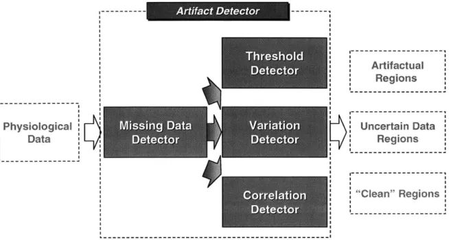
underlying physiological state of the patient, and in this way assign a level of user confidence in the data. More specifically, as shown in Figure 1.6, the objective is to
upon current rules-based systems and include analysis of correlation between physiological signals.
V
VNoisy
Regions
Uncertain
Regions
"Clean"
Regions
Figure 1.6 shows a block diagram of the proposed artifact detector.
This project coincides with efforts to use the MIMIC database to develop wavelet algorithms in discerning trends for use in intelligent patient monitoring. Moreover, as was mentioned previously, knowledge of the underlying signal quality is important in any
type of patient monitoring system. The aim of this project is thus to aid subsequent analysis of physiological data by labeling regions so that following stages can then choose to ignore or accept regions based upon their "tag."
However, as this research is concerned specifically with data used for the wavelet trend analysis, actual waveform data will not be discussed. Trend data, as discussed in this paper, is defined as signal recordings measured once every minute. Though the focus
Physiological
Data
of this paper will be on the research applications of artifact detection with an emphasis on such trend data, any algorithms presented may also be applicable in a clinical setting or other instances where waveform data is used. In addition, the research described here is concerned mainly with artifact detection. While the actual removal or replacement of artifactual data will be briefly discussed, such research is beyond the scope of this paper.
The following chapter will provide a brief background into the physiological signals involved in this research. A method is then presented to examine these signals and their validity, and results with analysis will follow.
Chapter 2 -Physiological Signals 2.1 Signal Selection
A large number of physiological signals are recorded from patients during their stay in the ICU. As these recordings often last for periods ranging from many hours to days, analysis of each signal for all patients would be a daunting task. The first stage of this project was thus to select a subset of signals to be used in the development and testing of any potential algorithm. This selection process was followed by a review of numerous trend recordings of each selected signal in an effort to become acquainted with the many different types of artifacts possible in physiological data.
Signals were chosen in large part due to their value in discerning information about the underlying physiology of the patient. The research described here seeks to build upon current artifact detection algorithms by incorporating the interrelation of
signals, and thus signals were also chosen such that there was a high degree of correlation among them. Additional factors considered included the amount of patient data available for the respective signals as well as their inherent level of noise.
Four signals were initially chosen that adequately fulfilled these criteria: heart rate; arterial blood pressure; central venous pressure; diastolic pulmonary artery pressure.
Though this list was later narrowed to include only heart rate and blood pressure, all four signals are of great value. It is hoped that this project can be extended in the future, beginning most likely by reexamining central venous pressure and diastolic pulmonary
artery pressure. A brief description of each variable is thus given subsequently in this chapter.
2.2 Heart Rate
A patient's heart rate relates the frequency at which his heart beats and is measured in units of beats per minute (bpm). A normal adult has an average resting heart rate of approximately 70 bpm, though heart rate may rise as high as 180 bpm during exercise.14 Certain people, such as athletes, will experience lower heart rates as their hearts are able to pump a larger volume of blood during every beat. This volume is called the stroke volume.
The body can regulate the cardiac output -the amount of blood pumped by the heart each minute -by increasing or decreasing heart rate. The relationship between cardiac output and heart rate can be defined as follows:
(Cardiac Output) = (Heart Rate) x (Stroke Volume) 2.1
This equation is useful in understanding the effect of heart rate on blood pressure, a topic discussed later in section 2.3. In addition to heart rate, myocardial contractility, preload, and afterload affect the cardiac output. Though preload and afterload are not considered in this thesis, preload is reflected in CVP and DPAP recordings and will be discussed in brief at the end of this chapter.
A typical heart rate trend can include large "spikes" where the signal value may increase dramatically in a short amount of time. An example is shown in Figure 2.1. These sudden jumps may be attributable, for example, to either a double-counting in the ECG waveform where one QRS complex is misidentified as two, or to a sudden heart rhythm change. The former results in an artifactual heart rate value and does not reflect
the true state of the patient. However, as alluded to previously, this study will be performed using data collected from ICU patients. The task of identifying artifacts is more difficult with such data as seemingly artifactual regions may be due to abnormal conditions present in ICU patients. During these instances such spikes may be attributed to an actual underlying physiological condition. One cause for such an event in the heart rate recording could be atrial fibrillation.
Heart Rate Trend Data 160 150- 140- 130- 120-110 100 90 70-60' 10 15 20 25 Hours
Figure 2.1 shows a typical heart rate trend pattern from an ICU recording.
Atrial fibrillation, the most common abnormal heart rhythm, is an arrhythmia that occurs in various types of chronic heart disease. Under this condition, the atria, or upper chambers of the heart, do not contract and relax sequentially. The atria instead undergo a continuous, uncoordinated, rippling motion and are no longer in sync with the lower chambers of the heart. No constant interval occurs between successive QRS complexes resulting in an irregular heart rhythm that can reach up to 160 bpm.14'15
Any potential artifact detector must attempt to distinguish between these true physiological events from artifacts. This can be accomplished, in part, by examining the
activity of other signals closely associated with heart rate. A true event that alters the heart rate trend data should also be evident elsewhere in related physiological signals. Blood pressure has a high level of correlation with heart rate and is one such signal that
can be used to cross-check uncertain variations.
2.3 Arterial Blood Pressure
The arterial blood pressure (ABP) pulse is generated by flow from the heart into the ascending aorta. Ejection of blood into the aorta dilates the aorta and generates a pressure wave. This wave is then propagated to other arteries throughout the body.16 Figure 2.2 is shown again from section 1.1 to provide an example of a blood pressure waveform recording.
1 5 0 Systolic ABP 1 4 0 1 30 1 2 0 1 3 0 9 0 80 7 0 Diastolic AB 7 137. 05 13 7 1 137. 15 137 2 m In u te s
Figure 2.2 shows a blood pressure waveform from an ICU recording.
The maximum value during each cycle is the systolic blood pressure whereas the minimum value is the diastolic blood pressure. The difference between the systolic and diastolic ABPs is defined as the pulse pressure. The average value over one cycle is the mean blood pressure. This value is a running average calculated independently from the systolic and diastolic measurements. A typical value for systolic ABP in a resting adult is
120 mmHg, 80 mmHg for diastolic ABP, and 90 mmHg for mean ABP.
The mean blood pressure and flow in the cardiovascular system follow a form of Ohms law, namely
MABP = (CO) (R) 2.2
where cardiac output (CO) is as defined by equation 2.1 in section 2.2 and R is the peripheral resistance. While frictional resistance is relatively small in the large arteries,
small arteries offer moderate resistance to blood flow. This resistance reaches a maximum in the arterioles. The pressure drop is greatest here across the terminal segment of the small arteries and the arterioles. The body is able to control the value of R by adjusting the degree of contraction of the circular muscle of these small vessels. This not only permits regulation of tissue blood flow but also aids in the control of arterial blood pressure. Equation 2.2 applies to both the systemic and pulmonary circulations.
Substituting for CO in the previous equation we arrive at
MABP = (HR x SV) (R) 2.3
Here, one begins to see the relationship between heart rate and blood pressure. This equation is applied, for example, as the cardiovascular system attempts to keep MABP constant using certain feedback mechanisms throughout the body. Changes in arterial blood pressure initiate a reflex that leads to an inverse change in heart rate and peripheral
resistance. If MABP is lowered, it follows from equation 2.3 that raising any
combination of HR, SV, and R, will cause a normalizing effect on MABP. This reflex is initiated, in part, by the baroreceptors.
The baroreceptors are stretch receptors located in the carotid sinuses and in the aortic arch. The pressoreceptor nerve terminals in the walls of the carotid sinus and aortic arch respond to the stretch and deformation of the vessel induced by the arterial pressure. With an increase in blood pressure, the frequency of impulses arising from the receptors also increases. The brainstem responds by decreasing sympathetic outflow while increasing parasympathetic outflow. The decreased sympathetic tone results in vasodilation and a drop in cardiac contractility. The resulting lowered heart rate is
reduced further by the changes in parasympathetic tone. Blood pressure therefore decreases due to the decrease in both cardiac output and in peripheral resistance in accordance with equation 2.2. The arterial baroreceptors thus play a key role in short-term adjustments of blood pressure in response to relatively abrupt changes in blood volume, cardiac output, or peripheral resistance.14
The role baroreceptors play in the regulation of blood pressure can be seen in the body's response to a hemorrhage. An individual who has lost a large quantity of blood
experiences a weak arterial pulse as the arterial systolic, diastolic, and pulse pressures decrease. The reduction in MABP and in pulse pressure during a hemorrhage decreases the stimulation of the barorecptors. As a result, several cardiovascular responses are evoked. Heart rate is increased and is accompanied by a related venoconstriction and arteriolar constriction. The resulting increase in peripheral resistance further minimizes the fall in arterial pressure. Figure 2.3 provides an illustration of the effect of
Figure 2.3 shows the effect of the baroceptors after an 8% blood loss in three groups of dogs. (A) shows the resulting blood pressure decrease in dogs where the aortic reflexes were interrupted. (B) shows the resulting blood pressure decrease in dogs where the carotid sinus reflexes were
interrupted. (C) shows the resulting blood pressure decrease in dogs where all baroreflexes were interrupted. 14
This response to hemorrhage further demonstrates the relationship between MABP and HR as described in equation 2.3. It should be noted, though, that the baroreceptor reflex is a feedback mechanism, and there will thus be a necessary corresponding error term associated with the blood pressure. Though heart rate and peripheral resistance result in an increased blood pressure, blood pressure does not return exactly to its pre-hemorrhage level. The net effect, factoring in the initial drop in blood pressure due to the blood loss, is a drop in blood pressure accompanied by an increase in
heart rate and peripheral resistance.
Nevertheless, holding other variables constant, if HR increases and there is no corresponding decrease in stroke volume, cardiac output and thus MABP should
between HR and MABP can be useful in determining the validity of data such as that in Figure 2.1. Following from equation 2.3, the large increase in the heart rate recording, if
it accurately portrays the patient's state, should also be evident, in some form, in the blood pressure recording. Unfortunately, there are instances where blood pressure will
fall even as heart rate increases, and other physiological data must also be taken into account.
A sudden rise in heart rate may be due to an onset of tachycardia, or an increase in the contraction frequency of the heart. In the case of supraventricular tachycardia, heart rate can suddenly reach up to 140 to 250 bpm. Such rapid contractions may not allow sufficient time for ventricular filling, and the heart is no longer able to function properly. Blood is no longer effectively being pumped into the body, and such situations can be accompanied by an exponential drop in blood pressure towards Pms -the mean systemic filling pressure. This is the pressure if there were no flow in the circulatory system.14
The difficulty in detecting artifacts lies in the fact that there are many causes for events, whether true or false in nature. Using the relationship between signals is helpful in determining the validity of a particular data set, but the complex interworkings of heart rate and blood pressure help illustrate that a thorough understanding of these relationships is needed. Further compounding the problem is the fact that associated variations, in and of themselves, do not necessarily indicate true and uncorrupted data.
Certain cases of artifactual noise pertain to a single signal. For example, a faulty electrode/lead will cause false heart rate recordings while the other signals will be unaffected. However, other situations may affect multiple channels. A patient coughing or moving may shift both the heart rate as well as the blood pressure recording though the
patient's underlying physiology remains unchanged. Again, any potential artifact detector must attempt to distinguish between these and true physiological events.
Lastly, just as heart rate and blood pressure are related, the individual components of blood pressure are also interrelated. Systolic, diastolic, and mean ABPs are positively correlated with each other as a change in one signal is usually accompanied by a similar change in the remaining two. Though these changes may not be of the same magnitude, an increase in the MABP should result in an increase in both the systolic and diastolic ABP, as well. If the stroke volume is increased by a factor of two while HR and R are held constant, equation 2.2 shows that MABP should similarly double in value. Under constant compliance, this increase in stroke volume will increase systolic and diastolic ABPs, but the systolic pressure will increase more so such that the pulse pressure will be approximately twice as great as before. Figure 2.4 shows a patient trend recording for heart rate and the individual blood pressure measurements.
Heart Rate Trend Data 140- 130-120 110 -0100 90 80 70 135 140 145 150 155 160 165 170 Hours
Blood Pressure Trend Data 160 140 120 E 100-E 40 135 140 145 150 155 160 165 170 Hours
Figure 2.4 illustrates the relationship between heart rate and blood pressure. In general, variations in the trend data shown here are evident in both the heart rate and blood pressure recordings. Notice, also, that there is a much higher degree of correlation between the systolic, mean, and
diastolic blood pressures than between the heart rate and blood pressure.
2.4 Central Venous Pressure (CVP)
Central venous pressure is the pressure in the right atrium and thoracic venae cavae and indicates the pressure of the blood as it returns to the right side of the heart. An
approximation of right ventricular end diastolic pressure, or right ventricular preload, CVP reflects right ventricular function. On average, CVP is around 1.5 mmHg but can range from just above OmmHg to 5mmHg. The recording shown in Figure 1.4 is thus unusually high, though that is indicative of many patients in an ICU.
CVP is closely linked to blood pressure in that it also affects cardiac output. This relationship, however, is defined by two functions -the cardiac function curve and the
vascular function curve. The cardiac function curve describes the effect of venous return on cardiac output and depends upon the characteristics of the heart. The vascular
function curve describes the effect of cardiac output on venous return and depends upon the characteristics of the vascular system. Though beyond the scope of this thesis, the actual value of CVP and cardiac output depend upon the intersection of these two curves.
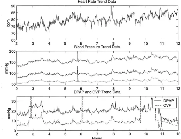
Figure 2.5 shows a central venous pressure trend pattern from an ICU recording alongside other recordings of interest.
2.5 Diastolic Pulmonary Artery Pressure (DPAP)
Diastolic pulmonary artery pressure is used to approximate the value of filling pressure of the left heart, or the end-diastolic pressure. Similar to CVP and its relationship to the right ventricle, DPAP is a measure of left ventricular preload. A normal value of DPAP for resting adults is around 9 mmHg
Figure 2.5 shows a diastolic pulmonary artery pressure trend pattern from an ICU recording alongside other recordings of interest.
2.6 Summary
The physiological signals presented here are interrelated with each other. These
relationships, if properly understood, can be used to enhance artifact detection in each of the signals. Though figure 2.5 illustrates numerous trend recordings for an ICU patient, henceforth the focus will remain solely on heart rate and blood pressure signals.
Heart Rate Trend Data
SI
I I- I
2 3 4 5 6 7 8 9 10 11 1
Blood Pressure Trend Data
2 3 4 5 6 7 8 9 10 11 1
DPAP and CVP Trend Data
3 4 5 6 7 8 9 10 11 1
Hours
Figure 2.5 shows the various trend data recordings for a particular individual. Note how variations in certain signals are evident in other signals, as well. Note also how there are instances where such a
relationship is not clearly seen.
2 2 2 90 85 75 70 65 200 om150 E E 100 50 30 r 20 E 10 I I I I I I I I I 1> I 1 I I I I I -0 2 DPAP -CVP )AA I W N I p I |
Chapter 3 -Artifact Detector Algorithm 3.1 Algorithm Overview
Many different types of artifacts exist in trend data, and only a few examples have been presented thus far. As shown in the previous chapters, certain instances of artifacts are
simple to identify while others are not as easily detected. This wide variety of noise presents a problem in that any algorithm used to detect artifacts must be robust enough to
recognize a large proportion of noise yet be fine-tuned enough to distinguish true events caused by a patient's underlying physiological state. The goal of the algorithm to be described here in this thesis to "tag" each region of physiological trend data from patients contained in the MIMIC database as one of three categories: reliable and clean of
artifacts; uncertain; definitely corrupted by noise.
The algorithm has been, to this point, presented as a black box. This chapter will discuss the artifact detector shown in Figure 1.6 in more detail. Figure 3.1 shows the artifact detector separated into its four components: missing data detector; threshold detector; variation detector; correlation detector. The following sections of this chapter will each discuss various types of artifacts, describe a particular subsection of the algorithm, and explain how it is designed to identify such artifacts.
In general, save for the missing data detector, each subsection is distinct from one another. The outputs from all detectors consist of regions where data has been tagged as uncertain and regions where data has been tagged as corrupted. These tags are then combined to create an aggregate set of uncertain and corrupted locations. Regions of data not tagged as either uncertain or corrupted are tagged as clean.
Physiological s D ra n Data . . . . ... .... .... .| Artifactual Regions Uncertain Data Regions "C-"---"Clean" Regions
Figure 3.1 expands figure 1.6 and depicts the aggregate artifact detector with its subsections: missing data detector; threshold detector; variation detector; correlation detector.
3.2 Missing Data Detector
Missing data in a recording is an easily identifiable class of artifact, and this lack of data may be attributed to any number of causes. A nurse may have disconnected the probe for the respective signal or there may have been a bad connection either to the patient or to the monitor. The function of the missing data detector in this project is twofold -it detects and stores locations of missing data and then "fills in" those regions.
Periods where no data is recorded are displayed differently based upon the devices being used to measure and collect the signals. The method to be described here is unique to the patient trend data stored in the MIMIC database. However, similar methods can be designed for different record formats if the manner of recording missing
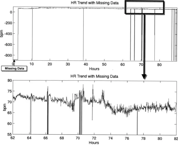
-888. Such a value is far beyond the possible range of any physiological signal and is thus easy to detect. Figure 3.2 provides an example of a recording with missing data.
0 -200 9--400 -600 -800 80 75 70 65-60L 10 20 30 40 50 60 70 80 ng Data Hours
HR Trend with Missing Data
II I I I I
62 64 66 68 70 72 74 76 78 80
Hours
Figure 3.2 shows a heart rate trend recording containing missing data. Notice the large section of missing data in the beginning compared to the smaller segments throughout the remainder of the recording. Figure (bottom) shows an expanded region from the recording. The regions of missing data differ greatly from those where data exists.
82
The detector locates regions of missing data by searching for all points in the trend recording of the value -888. Each instance is tagged as corrupted, and its time stamp is saved and passed on to be combined with artifact locations as determined by the other subsections of the algorithm. The missing data detector then replaces each instance of a -888 value in the trend data with an estimated value.
HR Trend with Missing Data
El
The question arises as to whether or not areas with missing data should be "filled in" and, if so, by what process should this be done. This study has chosen to use
substitute values in order to provide usable data for calculations in subsequent parts of the artifact detector. Certain stages following the missing data detector perform calculations on data over a window of time. While large sections of missing data (specifically those much larger than that of the window size) will not be worthwhile to pass through to
subsequent detectors, the algorithm currently does not limit the size of a missing data region to be filled in. However, the substitution process is most beneficial when smaller portions of data, those proportional in length to the window size, are missing. In such
cases, as in the absence of a single data point, calculations involving the area of noise and its surrounding data may not be possible, thus leading to the entire area within the
window to be declared artifactual.
A "best guess" for the missing data is thus used, and this estimate is determined using linear interpolation. The missing data detector takes note of the last true data point that is recorded before the section in question and the first true data point recorded afterwards. These two endpoints are used as a basis for linear interpolation, and the missing data is replaced with values from the resulting line between these two points. Instances of missing data that occur either at the beginning or end of a patient record do not provide a suitable beginning or end point for use in such a calculation. During these cases, a NaN value is substituted for the missing data, and no estimated values are passed on to following sections of the algorithm. The NaN value indicates in the mathematical program used for this thesis that there is "not a number" at that location. Further calculations around this region will not be possible.
Limitations to this method arise as physiological signals are inherently nonlinear. Linear interpolation thus, in and of itself, produces artifacts. Nevertheless, the resulting
artifacts should be minimal in the short-time-period situations where this method is most beneficial. Future work may attempt to study additional methods for managing missing data. The process for missing data detection is illustrated in figure 3.3.
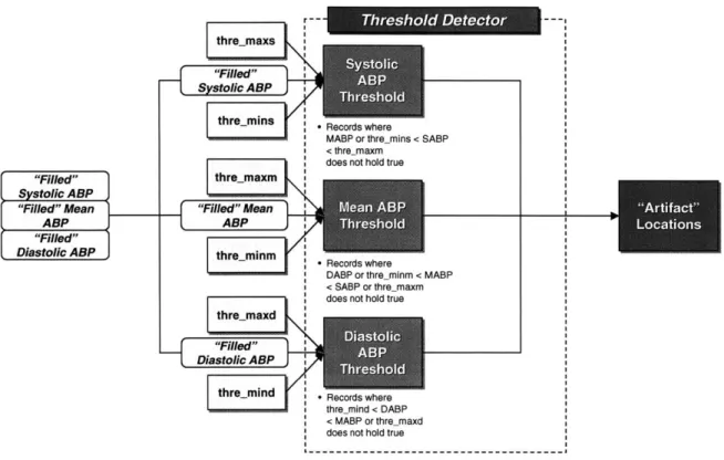
Missing Data Detector
Systolic ABP
Mean ABP
Diastolic ABP
Records where SABP = -888 and interpolates data for such areas y"Filled" sstolicAn :j"Filled"Mean ABP Records where MABP = -888 and interpolates data for such areas "Filled" DiastolicAB e Records where DABP = -888 and interpolates datafor such areas
Figure 3.3 shows a block diagram of the missing data detector. Though heart rate is not displayed here, it is filtered using the same methodology.
3.3 Threshold Detector
The preceding section introduced the situation where a physiological signal exhibited extremely low values, notably that of -888 during regions of missing data. Other values
in physiological trend data. More common in recordings are values that go above possible bounds, as shown in the sudden large step increase of CVP in figures 1.4 and
1.5. However, as CVP values are normally near zero, shifts in body position that can
affect the signal's baseline may result in negative CVP values. The reliability of such a data point is highly questionable. These artifacts, where values exceed either the
maximum or fall below the minimum thresholds of physical limitation, are, as with missing data, simple to detect.
The threshold detector receives as inputs two parameters in addition to the trend data to be analyzed. The user must specify a maximum value and a minimum value with relation to each signal. These values may be a constant value or that of another signal. Figure 3.4 provides an example of a blood pressure trend recording passed through the threshold detector as well as the resulting output tags.
BP Trend with Threshold Detection
X3200 E
20 25 30 35 40 45 50
1 -_Systolic ABP Threshold Det
i
-f I
1 ____Mean ABP Threshold Detection
0
20 25 30 35 40 45 50
1 1
1 Diastolic ABP Threshold Detection
0
20 25 30 35 40 45 50
Hours
Figure 3.4 (top) is a blood pressure recording showing systolic, mean, and diastolic blood pressures.
The remaining sections show the result of passing these through the threshold filter. Note how
regions where, for example, the systolic blood pressure falls below the mean blood pressure are tagged as artifactual by both the systolic and mean detectors.
The mean pressure, by definition, cannot exceed the systolic blood pressure or fall below the diastolic blood pressure. However, as the mean blood pressure is calculated
independently of systolic and diastolic measurements, an artifact in the systolic blood pressure signal may not appear in that of mean blood pressure. Though certain physiological conditions result in all three values being of similar magnitude, it is reasonable to set the maximum threshold for the mean blood pressure to be the systolic blood pressure and the minimum threshold to be the diastolic blood pressure. In addition,
used to address situations where either the systolic or diastolic blood pressure is artifactual and thus cannot provide a good basis with which to check the mean blood pressure.
The threshold detector locates all regions where the mean blood pressure exceeds either the systolic blood pressure or the maximum constant threshold, and it likewise locates regions where it falls below either the diastolic blood pressure or the minimum constant threshold. A similar process is applied to the systolic and diastolic blood pressures, and all time stamps of regions where values exceed their associated limits are tagged as corrupted. This set of locations is later combined with those similarly tagged by other detectors. A diagram of this process is provided in figure 3.5.
The difficulty with the threshold detector is the same as that of other rule-based filters described in chapter 1. Any maximum threshold must be set high enough to allow for actual physiological readings that are abnormally high but low enough to filter out areas that are not physiologically possible. Determining thresholds requires a thorough understanding of the signals themselves. Consequently, the values used in this project were chosen after a review of the literature, discussion with experts, and analysis of sample data.
-- Threshold Detector --thre maxs
"Filled"
SSystolic ABP
thre-mins .Records where
MABP or thre mins < SABP
< thre maxm
does not hold true
"Filled"o thre_maxm
Systolic A BP
"Filled" Mean"Fld"Mn-- *
ABP
ABP-"Filled"
'Diastolic ABP thre minm R cordwhr
DABP or thre_.minm < MABP
S< SABP or thre maxm
does not hold true thre-maxd
"Filled"dosn'o Diastolic A BP
thre mind -Record where
t rmhre_mind < DABP
< MABP or thre-maxd
does not hold true
Figure 3.5 shows a block diagram of the threshold detector as applied to blood pressure.
3.4 Variation Detector
Sections 3.2 and 3.3 presented two methods for detecting artifacts. However, a large number of artifacts that are not encompassed within the missing data category lie within reasonable physiological bounds. Certain such artifacts can be detected in a manner similar to that used by the threshold detector. Just as a blood pressure trend recording at any point in time cannot exceed a certain value, the change in blood pressure from one value to the next also cannot exceed a certain value. Though the mean blood pressure of a patient in an ICU can rise above 250 mmHg, it is not likely to do so if its value a minute earlier was below 100 mmHg. These spikes in value can be common in physiological recordings, and more advanced methods than the ones previously described are needed to detect such artifacts.
The variation detector searches for regions where there may be unreasonable changes in signal values by performing a moving standard deviation calculation over a set of trend data. Similar to the median filter described in chapter 1, the detector
calculates the standard deviation for each point and a "window" of points around it. This window slides over the entire data set until the standard deviation around each point is calculated. The result is a data set of standard deviations, one for each point in the corresponding trend data recording. This new set of standard deviation data will
henceforth be referred to as movstd. The overall standard deviation and mean of movstd are then calculated.
varwin "Filled" Systolic ABP var-win "Filled" Systolic A BP
"Filled" Mean ' Filled" Mean
ABP )ABP "Filled" Diastolic ABP "ied" Diastolic ABP --- Vai-n Detectr -var lim cons
-Calculates moving std of -Records where SABP SABP over a window standard deviation > size var win; Calculates min(var limmuls*STD + the STD and MEAN of MEAN var limcons this movin std var lim
conm
variim Mulm
Calculates moving std of * Records where MABP
MABP over a window standard deviation > size var win; Calculates min(var-limmulm*STD the STD and MEAN of MEAN, var limconm)
this moving std
var cond
-
rh~~var~Limmulm
varwin * Calculates moving std of * Records where DABP
DABP over a window standard deviation >
size var win; Calculates min(varJimmuld*STD + the STD and MEAN of MEAN, var-limcond)
- - -this moving std
Figure 3.6 shows a block diagram of the variation detector. Though heart rate is not displayed here, it is filtered using the same methodology.
1
---The variation detector, as shown in figure 3.6, receives three sets of parameters in addition to the trend data to be analyzed. The user must first specify a window size, varwin, for the moving standard deviation calculations. This input may be a vector containing multiple values, thus allowing for the detector to perform variation analysis over more than one window size. Larger windows allow for analysis of slower variations in the signal that may not be detected with smaller windows. Determination of window size is discussed in section 4.4.
Varlimmul, a user-defined constant, is then used to calculate a limit for determining regions of excess variation. The threshold for each signal is calculated using the following formula
(standard deviation of movstd) * varlimmul + (mean of movstd) =
threshold-variable 3.1
where movstd = moving standard deviation calculation of signal in question
and varlimmul = user-defined constant
The standard deviation of movstd is multiplied by varlimmul, and this value is added to the mean of movstd. The resulting threshold-variable is compared against each value of movstd, with those values exceeding it being tagged as artifactual. In this way, the variation detector searches for regions of unusual deviation, where the standard for variation is determined in relation to each individual patient. Statistical variables, specifically those of standard deviation and mean, are unique to a specific patient and thus allow the detector to define variation thresholds better suited to each patient.
Varlimcon, a maximum threshold value, is used to address situations where there may be extreme outliers in the data set. These outliers may raise the standard deviation
of movstd so high such that the value of threshold-variable is likewise very high. In these instances no regions besides that of the outliers are tagged. The actual threshold for variation is thus the minimum of threshold-variable and the varlimcon. Both varlimmul and varlimcon differ for heart rate and for blood pressure.
Figures 3.7 and 3.8 show the calculations and output of the variation detector. A final step is used to further verify the blood pressure data. As was noted in equation 2.3, blood pressure is correlated to heart rate. Any large or sudden change in blood pressure should somehow also be reflected in the heart rate. In the case of
ventricular fibrillation, when blood pressure drops exponentially within seconds, there is no coherent contraction of the heart and thus no ejection of blood. A variation in the heart rate is thus accompanied by a variation in the blood pressure.
Regions of blood pressure that have been tagged by the variation detector are thus checked with the corresponding regions in the heart rate trend data. If the variation detector has likewise tagged the heart rate, then the region is labeled as uncertain. The region is not labeled as clear due to the fact that, as described in section 2.3, associated variations do not in and of themselves fully indicate that the recordings are uncorrupted.
Regions with no corresponding tag in the heart rate recording are labeled as artifactual, and the remaining regions are labeled as clear. The time stamps of each set -uncertain, artifactual, and clear -are passed on and combined with those as tagged by other detectors.
BP Trend with Vaiation Detection :1200 E EV 0 20 25 30 35 40 45 50 50-A
Var-Lim-Con for SABP Var-Um-MuI*STD+Mean
25
~i!LIAdJLMA~*
~~KLL~ h~LA 1 ~30 35 40 45 50
50
Var-Lim-Con for MABP Var-Lim-Mul*STD+Mean
0 25-A.i
20 25 30 35 40 45 5
50
-Var-Lim-Con for DABP Var-Lim-MuI*STD+ Mean
0
20 25 30 35 40 45 50
Hours
Figure 3.7 shows the output from the first stage of the variation detector. The blood pressure trend recordings are passed through and the moving standard deviations for each signal are calculated. The solid horizontal line indicates varjlimcon, the maximum constant value, and the dashed horizontal line indicates threshold-variable as calculated using equation 3.1
BP Trend with Variation Detection
r'3200 E
0
20 25 30 35 40 45 50
1 -Systolic ABP Variation Detection
F, II II 111 1 1
0
20 25 30 35 40 45 50
1 Mean ABP Variaton Detection
j
30-350.
20 25 30 35 40 45 50
1 IDiastolic ABP Variation Detection
M, I
0)
20 25 30 35 40 45 50
Hours
Figure 3.8 shows the regions of blood pressure data that exceed either the constant threshold or threshold-variable. These regions are then tagged and compared with the heart rate recording.
3.5 Correlation Detector
Further analysis of artifacts requires a deeper understanding of physiology beyond checks against maximum values, minimum values, and maximum variation. This can be done through the incorporation of relationships between physiological signals. Current patient monitors make use of single-signal analysis and, as mentioned in chapter 1, this has proven to be a less-than-ideal solution. Though the variation detector made use of
inter-signal rules to account for relationships among recordings, this was limited to identifying if other signals had likewise been tagged as potentially corrupted. As such, the
verification of blood pressure variation based on heart rate variation was used more as an additional check than as an actual stand-alone detector. More subtle artifacts would pass through this system undetected.
A clot in a catheter with a transducer measuring blood pressure produces a recording such that the mean blood pressure value remains steady while the diastolic and systolic blood pressure values both begin to approach the mean. The clot thus acts as a low pass filter of the blood pressure signal. Figures 3.4 and 3.8 illustrate a potential clot around the 35th hour in the recording. Though this individual recording experiences high variation during this time, as shown in figure 3.8, were the transition of the diastolic and systolic values somewhat smoother, none of the aforementioned detectors would tag this region as artifactual. More robust analysis can be used in such cases involving highly correlated signals.
The correlation detector is the most complex of the subsections of the algorithm and performs a moving cross-correlation calculation over the trends of multiple signals from a single patient. With regards to blood pressure, the correlation detector calculates the correlation between the diastolic blood pressure and mean blood pressure, diastolic blood pressure and systolic blood pressure, and the correlation between mean blood
pressure and systolic blood pressure. These values are then examined to detect any changes in the relationship of these three signals.
Similar to the variation detector, the user must specify a window size, cor win, for the moving correlation calculation. This input may be a vector containing multiple values in order to detect changes over varying amounts of time. Correlations are
The user must also specify above what percentage of window-size-runs must a region be tagged to be considered artifactual.
Consider an example where the window size input is "[5 10 15]" and the
percentage input is ".5". This indicates that window sizes of 5 minutes, 10 minutes, and 15 minutes are to be used in calculating correlation between the blood pressure signals. Suppose a region is tagged during the 5-minute window calculation but is declared clear during the calculations of other window sizes. It has been tagged by less than half of window-size-runs, and the region is thus labeled as uncertain. Suppose another region is tagged during the 5 minute window calculation as well as during the 10 minute window calculation. This region has been tagged by two-thirds of the window-size-runs, greater than the 50% necessary, and this region is thus labeled as artifactual.
Regions of low correlation are determined by examining the absolute value of the difference between the three cross-correlation values. This is done using the following equation:
|correlation of diastolic and mean -correlation of diastolic and systolic| + Icorrelation of diastolic and mean -correlation of mean and systolicl + Icorrelation of mean and systolic -correlation of diastolic and systolicl=
correlation difference index (CDI) 3.2
This correlation difference index is calculated for each time period in the trend data and increases as the signals become less correlated. The correlation coefficient of each blood pressure signal with one another should normally equal one. In such cases, the difference between correlations would be zero, and the resulting CDI would also equal zero. This does not hold true during instances of corrupted data.
The mean blood pressure is determined independently of both systolic and
diastolic measurements. It is thus common for an artifact to exist either only in the mean blood pressure recording, or only in both the systolic and diastolic recording. In such cases, the correlation coefficient between the mean blood pressure and both the systolic
and diastolic blood pressures would fall well below one and the CDI value would increase. A similar situation occurs during the clot as described in the beginning of this section. The clot results in reduced correlation coefficients with regards to all three blood pressure signals.
The correlation detector compares each CDI value in a manner similar that used by the variation detector, namely the threshold-value is calculated as follows
(standard deviation of CDI) * var-limmulCDI + (mean of CDI) =
threshold-variableCDI 3.3
where CDI = correlation difference index as defined by equation 3.2
and varlimmul_CDI = user-defined constant
The overall standard deviation of CDI is multiplied with varlimmulCDI, a constant specified by the user, and added to the overall mean of CDI. This resulting value is compared against each value of CDI. Those values that exceed either this threshold or an additional user-inputted maximum constant value, varlimconCDI, are tagged. The determination of the tag, whether artifactual or uncertain, is based on the window-size-run percentage as described earlier.
A problem arises during regions of low variability within the signal. Correlation measures the degree of linearity between signals and is highly sensitive during periods when the signal values are relatively constant over a period of time. A small change in
only one such signal will result in a large change in its correlation value with other signals. Though this may be a normal phenomenon, the large change in correlation will result in the region being inappropriately tagged as corrupted. The correlation detector thus filters out regions of low variability and does not tag any data within these regions. The user specifies a set value for the underlying signal's standard deviation below which the correlation detector's output is disregarded.
The correlation detector thus receives five inputs: window size values; window-size-run-fraction; constant value to be multiplied by the standard deviation of CDI to calculate threshold-variableCDI; maximum constant value for CDI variation; minimum constant value for variation among the underlying signals. Note that the correlation detector does not attempt to determine which of the three blood pressure recordings contain artifacts, only that at least one of them is corrupted. Its output is saved and combined with those of the preceding subsections during the final step of the algorithm.
Figure 3.9 illustrates the correlation detector, while figures 3.10, 3.11, and 3.12 show a sample of patient data processed by the detector.
--- C--- DIeco
C O r-wi n --9-9
---"yiled" From Variation
S stoic i -DetectorI AS Calculates the
correlation coefficients
for the systolic ABP over Cor std Corim
COr win a window of size cor-win
SystolReord
wher the-wi
a idwoIiecr,
'"Fillcre "Filled" Meanoe tan
Diastolic ABP
Calculates the Sums up the absolute Filters out the time correlation coefficients value of the differences periods where the
for the mean ABP over a in correlation at each standard deviation of all:
Window of size cor-win point in time ABP's are less than cor-std
eRecords where the difference is above "Filled"cor-lim
Diastolic ABP
Corwin Calculates the
correlation coefficient~s
for the diastolic ABP over a window of size cor-win
BP Trend with Correlation Detection 300 250 -E E 50 0 2 1 0.5 0 -0.5 .4 0 20 25 30 35 40 45 50
Dotted -SABP/MABP Cor; Solid - SABP/DABP Cor; Dashed - MABP/DABP Cor
25 30 35
Hours
40 45 50
Figure 3.10 shows the output from the first stage of the correlation detector. Figure (top) displays the sample trend data, and figure (bottom) displays the correlation coefficients for the three signals. Note how correlation values change in areas where the blood pressure signals vary irrespective of
each other, as around the 35' and 4 0th hour. Note also how correlation values change in areas where
there is little variation in the signals though the blood pressure values seem to change in relation to each other, as after the 4 2"d hour.
- 4S
iw'Yt If (I j
&kF
~r~1liiv~I ~I ~~'
(,
200
150| 100
Dotted -SABP/MABP Cor; Solid -SABP/DABP Cor; Dashed - MABP/DABP Cor
0.5 t'
-0.5-
~ ~11I
J
ri*
-1
20 25 30 35 40 45 50
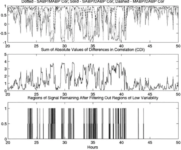
Sum of Absolute Values of Differences in Correlation (CDI) 5 4 3 2 1 0 20 25 30 35 40 45 50
Regions of Signal Remaining After Filtering Out Regions of Low Variability
1-
0.5-
0-20 25 30 35 40 45 50
H ours
Figure 3.11 (top) again shows the correlation coefficients, while figure (middle) displays the calculated CDI. Notice how the CDI is high during the regions of potential clots by the transducer, such as around the 3 5th and 4 0'h hours. Figure (bottom) shows the regions of the underlying signal,
Sum of Absolute Values of Differences in Correlation (CDI)
4-3
2-20 25 30 35 40 45 50
CDI in Regions of High Variability
Var-Lirn-Con for CDI
3- Var-Lim-Mul*STD+Mean
2
20 25 30 35 40 45 50
Blood Pressure Correlation Detection 1
-0
20 25 30 35 40 45 50
Hours
Figure 3.12 illustrates the final output of the correlation detector. Figure (top) again shows the CDI values, while figure (middle) displays the CDI values after those associated with regions of low variability have been removed. The dashed line represents threshold-variable. Note how in this case it is very high, and the user defined maximum constant value of var-lim-con is used instead.
3.6 Combined Detector
The output of each individual detector is saved and combined in the last stage of the algorithm. The regions labeled as artifactual from each detector are combined, as are regions labeled as uncertain by the variation detector and the correlation detector. This process is shown in figure 3.13. There is a degree of overlap among the outputs as more than one subsection may detect the same artifacts.