HAL Id: hal-02483552
https://hal-brgm.archives-ouvertes.fr/hal-02483552
Submitted on 18 Feb 2020
HAL is a multi-disciplinary open access
archive for the deposit and dissemination of
sci-entific research documents, whether they are
pub-lished or not. The documents may come from
teaching and research institutions in France or
abroad, or from public or private research centers.
L’archive ouverte pluridisciplinaire HAL, est
destinée au dépôt et à la diffusion de documents
scientifiques de niveau recherche, publiés ou non,
émanant des établissements d’enseignement et de
recherche français ou étrangers, des laboratoires
publics ou privés.
Simulating the Impact of Sea-level Rise and Offshore
Bathymetry on Embayment Shoreline Changes
Arthur Robinet, Bruno Castelle, Déborah Idier, Maurizio d’Anna, Gonéri Le
Cozannet
To cite this version:
Arthur Robinet, Bruno Castelle, Déborah Idier, Maurizio d’Anna, Gonéri Le Cozannet. Simulating
the Impact of Sea-level Rise and Offshore Bathymetry on Embayment Shoreline Changes. Journal of
Coastal Research, Coastal Education and Research Foundation, In press, pp.1 - 5. �hal-02483552�
____________________
DOI: 10.2112/SI95-0XX.1 received Day Month Year; accepted in revision Day Month Year.
*Corresponding author: [email protected]
©Coastal Education and Research Foundation, Inc. 2020
Simulating the Impact of Sea-level Rise and Offshore Bathymetry
on Embayment Shoreline Changes
Arthur Robinet†*, Bruno Castelle§
, Déborah Idier‡, Maurizio D’Anna‡§ and Gonéri Le Cozannet‡
ABSTRACT
Robinet, A.; Castelle, B.; Idier, D.; D’Anna, M., and Le Cozannet, G., 2020. Simulating the impact of sea-level rise and offshore bathymetry on embayment shoreline changes. In: Malvárez, G. and Navas, F. (eds.), Proceedings from the International Coastal Symposium (ICS) 2020 (Seville, Spain). Journal of Coastal Research, Special Issue No. 95, pp. 1–5. Coconut Creek (Florida), ISSN 0749-0208.
LX-Shore is a reduced-complexity shoreline change model driven by cross-shore and longshore processes which can account for man-made or natural non-erodible areas such as groynes and headlands. Here we describe and further test the implementation of two recent developments allowing to account for (i) real and non-erodible offshore bathymetric features such as rocky outcrops and canyons affecting offshore wave transformation and, in turn, shoreline variability and (ii) shoreline retreat due sea-level rise. After a description of the numerical developments, the benefits of these new developments are demonstrated with the application of LX-Shore to an idealized embayed beach exposed to real wave climate during a 10-yr period. Three simulations are conducted to test the impact of an outcrop in the middle of the embayment and of a gradual 1-m sea-level rise on shoreline spatial and temporal modes of variability. Results show that the equilibrium planview shoreline and the shoreline variability are strongly impacted by only slightly modifying the bathymetry and varying the mean sea level. These results show the potential of LX-Shore to better understand and further predict shoreline change along real coasts exhibiting mixed (sandy/rocky) and complex seabed morphologies and undergoing sea-level rise.
ADDITIONAL INDEX WORDS: Shoreline model, sediment transport, bathymetry, waves, sea-level rise.
INTRODUCTION
Worldwide, wave-dominated sandy coasts are subject to complex changes driven by a myriad of physical processes acting on a wide range of spatiotemporal scales (Vitousek et al., 2017). Although most of the physical processes are well characterized, accurately simulating shoreline changes along these coasts is still challenging. In the last decades, the development of a new generation of shoreline change models allowing predictions of past and future shoreline changes has received a growing interest from the scientific coastal community and coastal risk managers (Montaño et al., 2020). Physical-based reduced-complexity shoreline models focus on shoreline changes only and rely on the few processes that are dominant on the timescales from storm event to decades up to century. They are computationally cheap and robust.
However, reduced-complexity models usually oversimplify the bathymetry and/or the wave transformation processes. They cannot therefore account for the effect of complex seabed morphologies, sometimes observed along real coasts, that may impact the characteristics of onshore-propagating waves and, in turn, the nearshore sediment transports and shoreline changes. Recently Limber et al. (2017) coupled the Coastal Evolution Model (Ashton and Murray., 2006) with the spectral wave model SWAN (Booij et al., 1999) and included nearshore shoals in the bathymetry. They thus highlighted the control of the
seabed morphology on the equilibrium planview shoreline. However, their model only takes into account shoreline change driven by gradients in longshore transport.
Accounting for the sea-level rise (SLR) in reduced-complexity models is also crucial to tackle future shoreline changes on the timescales of decades and more (e.g. Vitousek et
al., 2017). Indeed, it is expected that sea-level rise will dominate
shoreline erosion by the end of the century (Le Cozannet et al., 2016). SLR may also affect the shoreline variability on shorter timescales in presence of complex offshore bathymetries, with increased depths potentially affecting offshore wave propagation, and, in turn, breaking wave conditions and sediment transport along the coast.
This contribution presents the numerical developments performed to integrate the above-mentioned processes in the state-of-the-art shoreline change model LX-Shore (Robinet et al., 2018). The benefits of these new developments are illustrated by applying LX-Shore to an idealized embayed beach exposed to a real wave climate during a 10-yr period.
METHODS Overview of LX-Shore
LX-Shore is a one-line-based reduced-complexity model resolving shoreline change driven by gradients in longshore sediment transport and by cross-shore processes resulting from disequilibrium between the instantaneous wave conditions and the recent past wave conditions to which the beach was exposed. The total longshore sediment transport is computed with the formula of Kamphuis et al. (1991) and the cross-shore processes are described by an adaptation of the ShoreFor model (Splinter
www.cerf-jcr.org
†
BRGM (French Geological Survey) Pessac, France
www.JCRonline.org
§Univ. Bordeaux, UMR CNRS 5805 EPOC Pessac, France
‡
BRGM (French Geological Survey) Orleans, France
2 Robinet, D’Anna, Castelle, Idier and Le Cozannet
_________________________________________________________________________________________________
Journal of Coastal Research, Special Issue No. 95, 2020
et al., 2014). LX-Shore does not resolve explicitly the
displacements of specific shoreline points, but instead relies on a 2D grid of cells containing sediment fraction values (ratio of dry to wet area in each grid cell) that are updated at the end of every simulation timestep (based on above-mentioned processes). The shoreline is then retrieved using an interface reconstruction method applied to this grid. LX-Shore is dynamically coupled with SWAN to ensure realistic and robust prediction of breaking wave conditions, which are then used to drive longshore and cross-shore processes. In the former version of LX-Shore (Robinet et al., 2018), sea-level rise was not taken into account and the bathymetry provided to SWAN was idealized and computed by LX-Shore at every simulation timestep using the approach of Kaergaard and Fresoe (2013), i.e. by imposing a stationary Dean-like beach profile seaward the simulated planview shoreline. Below we describe two recent developments.
Inclusion of Real Seabed Morphologies
One new development is the possibility to include real bathymetric features and to specify non-erodible bottoms in the bathymetry used by SWAN. If a measured bathymetry, hereafter referred to as the reference bathymetry (hr), is provided to
LX-Shore, it will be automatically merged with the idealized bathymetry (hi) originally computed by LX-Shore at every
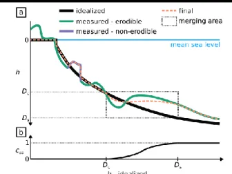
simulation timestep (Figure 1). This processing is based on two threshold depths, the depth of closure (Dc) and a tunable depth
(Ds) greater than Dc, and on the following rules: (i) hi is kept
near the shoreline, i.e. for 0 ≤ hi < Dc (Figure 1, black line); (ii)
hr is kept offshore, i.e. for hi > Ds (Figure 1, green line); (iii) a
merged bathymetry (hm) is computed and kept for Dc ≤ hi ≤ Ds to
ensure a smooth transition, based on the formulas:
hm = hi + (hr – hi) css (1)
css = 3 NDR2 – 2 NDR3 (2)
NDR = (hi – Dc) / (Ds – Dc) (3)
where css a sigmoid-shaped coefficient (function of hi, Figure 1b)
and NDR a normalized depth ratio ranging from 0 to 1. Lastly, the resulting bathymetry is compared to the reference bathymetry where the bottom is non-erodible (Figure 1, purple line). Adjustments can then be made to ensure that the final bathymetry never gets deeper than the bathymetry of non-erodible bottoms.
Inclusion of the Sea-Level Rise
A sea-level-change module has been implemented in LX-Shore to allow: (i) variations of the mean sea-level above the reference bathymetry initially provided to LX-Shore; (ii) shoreline retreat driven by SLR as predicted by the so-called Bruun Rule (Bruun, 1962). The first approach allows exploring how the shoreline dynamic is affected by changes in the characteristics of incoming waves due to variations of the mean sea-level. With the second approach, the planview shoreline will progressively retreat as the mean sea-level rises based on the following equation:
dS = dη / tan α (4)
where dS is the cross-shore shoreline retreat associated with the
sea-level rise dη and tan α is the average beach profile slope calculated between the shoreline position and Dc. Two important
assumptions are made: (i) the beach profile used to compute the idealized bathymetry remains the same; (ii) the mean-sea-level contour of emerged rocky structures remains the same as these structures are considered vertical and infinitely high.
Figure 1. Methodology used to merge the idealized bathymetry computed by LX-Shore with a measured bathymetry. Based on the idealized bathymetry, from 0 to Dc the idealized bathymetry is kept, from Dc to Ds the merging occurs and below Ds the measured bathymetry is kept. The bottom panel shows the sigmoid-shaped function used for the merging.
Test Case
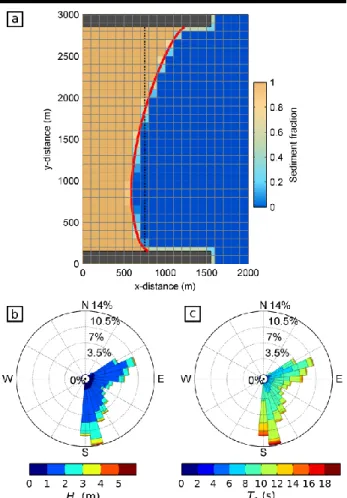
LX-Shore is applied to an idealized embayed beach (Figure 2a) whose characteristics and wave climate are inspired by those of Narrabeen beach (Sydney, Australia) (Turner et al., 2016). The model is forced with the wave conditions (Hs, Tp, Dp)
hindcasted at the Sydney buoy (Durrant et al., 2014) between 22/07/2005 and 22/07/2015. The tide is neglected and the shoreline position is assumed to correspond to the intersection between the mean sea level and the topography. The beach profile used to compute the idealized bathymetry was calibrated using the time and spatial average of bathymetric profiles measured at Narrabeen along cross-shore transects (transects PF2, PF4 and PF6 in Turner et al., 2016) down to nearly 14-m depth. Depth of closure was roughly estimated to 8 m using the formula of Hallermeier (1981) based on SWAN-simulated breaking wave conditions extracted at the center of the embayment. No hypothesis was made on the planview shoreline used to start the simulations. To obtain an initial shoreline in relative equilibrium with the wave climate a preliminary simulation (s0) is performed with LX-Shore using a straight N-S-oriented shoreline (Figure 2a, dotted black line) and enabling only the longshore sediment transport. The shoreline rapidly curves and rotates around a pseudo-equilibrium planview shoreline. The latter is taken as the initial condition of each simulations presented in the next section and is computed as the temporal average of the planview shorelines simulated from 2010-2015 in s0 (Figure 2a, red line).
Effects of Submerged Morphologies and Sea-Level Rise
Three simulations are conducted with different model configurations (Table 1) to illustrate the benefits of the new developments made in LX-Shore. In all simulations, both longshore and cross-shore processes are enabled. Breaking wave conditions extracted in the center of the embayment during simulation s0 and the cross-shore shoreline positions measured at the Narrabeen PF6 transect (Turner et al., 2016) from 2005 to 2015 are used to calibrate the free parameters of the cross-shore model using the methodology presented in Robinet et al. (2018). In simulation s1, the reference bathymetry provided to LX-Shore is the idealized bathymetry that LX-LX-Shore computes at the first timestep of the simulation (Figure 3a). Simulation s2 is similar to s1 but a Gaussian-shaped outcrop is added to the reference bathymetry in the center of the embayment (Fig 3b). This outcrop culminates in 6-m depth, has a diameter of nearly 500 m and lies in depths ranging from 12 to 25 m. Simulation s3 is similar to s2 but a constant SLR rate is applied throughout the simulation, which leads to a +1-m elevation of the mean sea level at the end of the simulation.
Figure 2. (a) Overview of the idealized embayed beach features and discretization adopted in LX-Shore. The red line denotes the initial planview shoreline used in all simulations. The dark grey patches denote the headland extents. The grid cell colors indicate the initial sediment
fraction for LX-Shore simulations s1,s2 and s3. (b,c) Wave rose of Hs and Tp, respectively, illustrating the wave climate used in all simulations
Table 1. Main characteristics of the simulations s1, s2 and s3. L and C refer to longshore and cross-shore processes, respectively.
ID L C Outcrop SLR
s1 yes yes no no
s2 yes yes yes no
s3 yes yes yes yes
Figure 3. Reference bathymetry used in simulations s1 (left panel) and s2-s3 (right panel). The red line denotes the starting shoreline used in all simulations. The dark grey patches denote the headland extents.
RESULTS Average Planview Shoreline
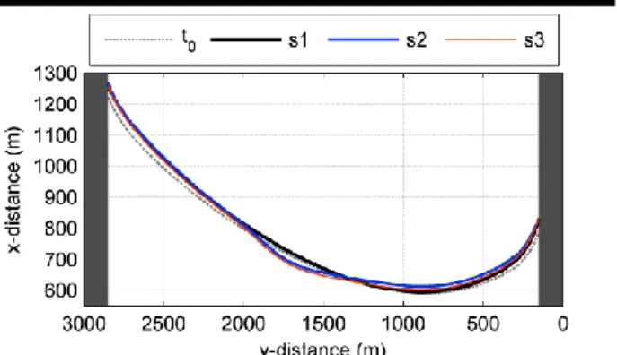
Figure 4 shows the initial planview shoreline (dotted grey line) and the averages of the planview shorelines simulated in s1 (thick black line), s2 (blue line) and s3 (red line). The overall shape of the averaged planview shorelines is similar, though substantial changes are visible between y = 0 m and y = 2000 m. The inclusion of the outcrop in simulation s2 led to an adjustment of the averaged planview shoreline with a mean shoreline retreat (progradation) of about 15 m for 1300 < y < 2000 m (y ≤ 1300 m) and a maximum retreat of 30 m near y = 1700 m. Although not clearly visible, the inclusion of the SLR effects in simulation s3 led to a shoreline retreat of about 10 m all along the beach.
Modes of Shoreline Variability
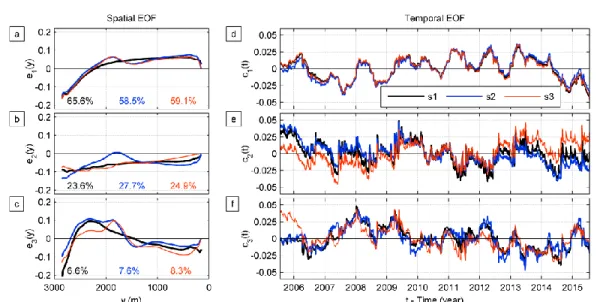
Following the methodology used in Harley et al. (2015), an Empirical Orthogonal Function (EOF) decomposition is applied to the demeaned timestacks of simulated planview shorelines to extract the three first spatiotemporal modes of shoreline variability simulated in s1, s2, and s3 (thick black lines, blue lines and red lines in Figure 5, respectively).
Interestingly, for simulation s1 the two first dominant modes are similar to those identified at Narrabeen in Harley et al.
4 Robinet, D’Anna, Castelle, Idier and Le Cozannet
_________________________________________________________________________________________________
Journal of Coastal Research, Special Issue No. 95, 2020 (2015). They are the beach rotation mode (black line in Figure
5a,d) related to longshore transport, and the beach translation mode (black line in Figure 5b,e) related to cross-shore transport and whose spatial magnitude decrease toward the south. The third mode, however, is different and seems here to correspond to a process of beach curvature variation resulting from transfer of sediments contained between 1500 < y < 2700 m to adjacent extremities on the timescales from storm event to years.
Figure 4. Initial shoreline (dotted grey line) used in all simulations and 10-yr averages of the planview shorelines simulated in s1 (black line), s2 (blue line) and s3 (red line).
The inclusion of the outcrop in simulation s2 induces significant changes mostly in the spatial component of the modes of shoreline variability (Figure 5a,b,c) essentially located near the center of the beach. One major change with respect to simulation s1 is the apparent attenuation of the translation process near yy = 1800 m (Figure 5b). The presence of this
outcrop also appears to slightly inhibit (increase) the contribution of the rotation (translation) mode to overall shoreline variability (Figure 5a,b).
The inclusion of the SLR effects in simulation s3 modifies essentially the spatiotemporal components of mode 2 and 3 (Figure 5b,c,e,f). The attenuation of the translation mode simulated in simulation s2 is removed (Figure 5b) and the trend
in the temporal component of mode 2 is reversed with respect to simulations s1 and s2 (Figure 5e).
DISCUSSION
Consistently with the philosophy of reduced-complexity models, simple and computationally cheap developments have been implemented in LX-Shore to account for the complex bathymetry and sea-level rise effect. Here, we presented a test case derived from the Narrabeen beach. A great similarity is found between the dominant modes of shoreline variability simulated by LX-Shore (s1 case) and those isolated at Narrabeen (Harley et al., 2015). Thus, despite its apparent simplicity, LX-Shore appears as a relevant tool to simulate shoreline dynamics and to explore the respective contribution of the physical processes involved in shoreline changes.
The comparative analysis of the results of simulations s1 and s2 suggests that the presence of the Gaussian-shaped outcrop at the center of the embayment modifies the average planview shoreline, which is consistent with the findings of Limber et al. (2017). The outcrop also appears to strongly impact the shoreline spatial and temporal variability, as evidenced by the changes in the spatial component of the dominant modes of shoreline variability. Although the shoreline dynamic is predominantly modified in the lee of the outcrop from a modal-wave-direction point of view (Figure 4 and 5), non-negligible adjustments are also induced elsewhere along the embayment (e.g. Figure 5b,c). These results suggest that the sea bottom morphology, and not only the combination of the wave climate and the headland sheltering, contributes to the shoreline dynamic along embayed beaches presenting complex bathymetries (e.g. presence of outcrops and/or submerged rocky platforms typically extending from headlands).
The sea-level rise also has a significant effect on the simulated shoreline variability. While the beach rotation mode appears to be insensitive to this process, this is not the case of the translation mode whose spatial component is similar to the spatial component of the translation mode obtained when the outcrop is absent from the bathymetry. The continuous increase
Figure 5. Spatial (a,b,c) and temporal (d,e,f) components of the dominant modes of shoreline variability isolated by applying an EOF decomposition to the timestacks of planview shorelines simulated in simulations s1 (thick black line), s2 (blue line) and s3 (red line).
sea level during the simulation may have damped the wave transformation processes occurring above the outcrop, resulting in more uniform wave conditions along the beach and in turns more uniform cross-shore processes. It is worth notifying that the temporal component of the translation mode is merely affected by the presence of the outcrop. However, the inclusion of the SLR effect leads to a reversal in the trend, which, combined to the shape of the spatial component, correspond to a progressive retreat of the coastline. While the SLR effect on the spatial component of the translation mode may be essentially related to the impact of variation of the mean sea level on wave transformation processes, the effect on the temporal component is likely to be the consequence of the application of the Bruun rule in LX-Shore.
Here, the assessment of the relevance of the new developments is based on an idealized test case without quantitative comparison to measurements. Future applications of the model will have to focus on assessing rigorously the model skill at real sites (e.g. Robinet et al., 2020) and the impact of calibration parameter uncertainties (e.g. D’Anna et al., in revision).
CONCLUSIONS
New developments were made in LX-Shore to further extend the range of possible real site applications. LX-Shore can now integrate real bathymetric features, which are shown to impact significantly the primary processes that drive shoreline variability. The model therefore appears as a promising tool to better understand and predict the respective contribution of the physical processes driving shoreline changes at sites exhibiting mixed (sandy/rocky) and complex seabed morphology. By extension, the model can also be used to anticipate the effects of building detached defense structures on shoreline variability, which are not necessarily confined to the vicinity of the structures. Finally, LX-Shore can now integrate SLR effects on the shoreline variability (through changes in wave transformation processes) and long-term retreat. This opens
perspectives for shoreline prediction on the timescales from storm event to century.
ACKNOWLEDGMENTS
The present work was funded by BRGM. The authors are grateful to the Water Research Laboratory team (University of New South Wales, Australia) which welcomed Arthur Robinet for a 3-month stay. Sydney wave data were kindly provided by the Manly Hydraulics Laboratory on behalf of the NSW Office of Environment and Heritage.
LITERATURE CITED
Ashton, A.D. and Murray, A.B., 2006. High-angle wave instability and emergent shoreline shapes: 1. Modeling of sand waves, flying spits, and capes. Journal of Geophysical
Research, 111.
Booij, N.; Ris, R.C., and Holthuijsen, L.H., 1999. A third-generation wave model for coastal regions: 1. Model description and validation. Journal of Geophysical
Research: Oceans, 104, 7649-7666.
Bruun, P., 1962. Sea-level rise as a cause of shore erosion.
Journal of the Waterways and Harbors division, 88(1),
117-132.
D’Anna, M.; Idier, D.; Castelle, B.; Le Cozannet, G.; Rohmer, J., and Robinet, A., (in revision). Impact of model free parameters and sea-level rise uncertainties on 20-years shoreline hindcast: the case of Truc Vert beach (SW France). Earth Surface Processes and Landforms.
Durrant, T.; Greenslade, D.; Hemer, M., and Trenham, C., 2014. A global wave hindcast focussed on the Central and South Pacific. CAWCR Technical Report, 70.
Hallermeier, R., 1981. A profile zonation for seasonal sand beaches from wave climate. Coastal Engineering, 4 (3), 253-277.
Harley, M.D.; Turner, I.J., and Short, A.D., 2015. New insights into embayed beach rotation: The importance of wave
6 Robinet, D’Anna, Castelle, Idier and Le Cozannet
_________________________________________________________________________________________________
Journal of Coastal Research, Special Issue No. 95, 2020 exposure and cross-shore processes. Journal of
Geophysical Research: Earth Surface, 120, 1470-1484.
Kaergaard, K. and Fredsoe, J., 2013. A numerical shoreline model for shorelines with large curvature. Coastal
Engineering, 74, 19-32.
Kamphuis, J.W., 1991. Alongshore sediment transport rate.
Journal of Waterway, Port, Coastal, and Ocean Engineering, 117 (6), 624-641.
Le Cozannet, G.; Oliveros, C.; Castelle, B.; Garcin, M.; Idier, D.; Pedreros, R., and Rohmer, J., 2016. Uncertainties in Sandy Shorelines Evolution under the Bruun Rule Assumption. Frontiers in Marine Science, 3, 49.
Limber, P.W.; Adams, P.N., and Murray, B., 2017. Modeling large-scale shoreline change caused by complex bathymetry in low-angle wave climates. Marine Geology, 383, 55-64.
Montaño, J.; Coco, G.; Antolínez, J.A.A.; Beuzen, T.; Bryan, K.R.; Cagical, L.; Castelle, B.; Davidson, M.A.; Goldstein, E.B.; Ibaceta, R.; Idier, D.; Ludka, B.C.; Massoud Ansari, S.; Mendez, F.J.; Murray, A.B.; Plant, N.G.; Ratliff, K.M.; Robinet, A.; Rueda, A.; Senechal, N.; Simmons, J.A.; Splinter, K.D.; Stephens, S.; Towned, I.; Vitousek, S., and Vos, K., 2020. Blind testing of shoreline evolution models,
Scientific Reports, 10, 2137.
Robinet, A.; Idier, D.; Castelle, B., and Marieu, V., 2018. A reduced-complexity shoreline change model combining longshore and cross-shore processes: The LX-Shore model.
Environmental Modelling & Software, 109, 1-16.
Robinet, A.; Castelle, B.; Idier, D.; Harley, M.D., and Splinter, K.D., 2020. Controls of local geology and cross-shore/longshore processes on embayed beach shoreline variability. Marine Geology, 422, 106118.
Splinter, K.D.; Turner, I.L.; Davidson, M.A.; Barnard, P.; Castelle, B., and Oltman-Shay, J., 2014. A generalized equilibrium model for predicting daily to interannual shoreline response, Journal of Geophysical Research:
Earth Surface, 119(9), 1936-1958.
Turner, I.L.; Harley, M.D.; Short, A.D.; Simmons, J.A.; Bracs, M.A.; Phillips, M.S., and Splinter, K.D., 2016. A multi-decade dataset of monthly beach profile surveys and inshore wave forcing at Narrabeen. Australia. Scientific
Data, 3(160024).
Vitousek, S.; Barnard, P.L.; Limber, P.; Erikson, L., and Cole, B., 2017. A model integrating longshore and cross-shore processes for predicting long-term shoreline response to climate change. Journal of Geophysical Research: Earth