Cloud-scale model intercomparison of chemical constituent transport in deep convection

(1)

HAL Id: hal-00328088

https://hal.archives-ouvertes.fr/hal-00328088

Submitted on 8 Jun 2007

HAL is a multi-disciplinary open access

archive for the deposit and dissemination of sci-entific research documents, whether they are pub-lished or not. The documents may come from teaching and research institutions in France or abroad, or from public or private research centers.

L’archive ouverte pluridisciplinaire HAL, est destinée au dépôt et à la diffusion de documents scientifiques de niveau recherche, publiés ou non, émanant des établissements d’enseignement et de recherche français ou étrangers, des laboratoires publics ou privés.

Cloud-scale model intercomparison of chemical

constituent transport in deep convection

M. C. Barth, S.-W. Kim, Chen Wang, K. E. Pickering, L. E. Ott, G.

Stenchikov, M. Leriche, S. Cautenet, J.-P. Pinty, Christelle Barthe, et al.

To cite this version:

M. C. Barth, S.-W. Kim, Chen Wang, K. E. Pickering, L. E. Ott, et al.. Cloud-scale model intercom-parison of chemical constituent transport in deep convection. Atmospheric Chemistry and Physics Discussions, European Geosciences Union, 2007, 7 (3), pp.8035-8085. �hal-00328088�

(2)

ACPD

7, 8035–8085, 2007 Cloud chemistry model intercomparison M. C. Barth et al. Title Page Abstract Introduction Conclusions References Tables Figures ◭ ◮ ◭ ◮ Back Close

Full Screen / Esc

Printer-friendly Version

Interactive Discussion

EGU

Atmos. Chem. Phys. Discuss., 7, 8035–8085, 2007 www.atmos-chem-phys-discuss.net/7/8035/2007/ © Author(s) 2007. This work is licensed

under a Creative Commons License.

Atmospheric Chemistry and Physics Discussions

Cloud-scale model intercomparison of

chemical constituent transport in deep

convection

M. C. Barth1, S.-W. Kim1,*, C. Wang2, K. E. Pickering3,**, L. E. Ott3,**,

G. Stenchikov4, M. Leriche5,***, S. Cautenet5, J.-P. Pinty6, Ch. Barthe6, C. Mari6, J. Helsdon7, R. Farley7, A. M. Fridlind8,****, A. S. Ackerman8,****, V. Spiridonov9, and B. Telenta10

1

National Center for Atmospheric Research, Boulder, Colorado, USA 2

Massachusetts Institute of Technology, Cambridge, Massachusetts, USA 3

University of Maryland, College Park, Maryland, USA 4

Rutgers University, New Brunswick, New Jersey, USA 5

CNRS/University Blaise-Pascal, Clermont-Ferrand, France 6

CNRS/Paul Sabatier University, Toulouse, France 7

South Dakota School of Mines and Technology, Rapid City, South Dakota, USA 8

NASA-Ames Research Center, Moffett Field, California, USA 9

Hydrometeorological Institute, Skopje, Macedonia 10

SENES Consultant Ltd., Toronto, Canada *

now at: ESRL/CSD and CIRES, University of Colorado, Boulder, Colorado, USA **

(3)

ACPD

Full Screen / Esc

EGU

∗∗∗_{now at: CNRS/Paul Sabatier University, Toulouse, France}

∗∗∗∗_{now at: NASA-GISS, New York City, New York, USA}

Received: 14 May 2007 – Accepted: 27 May 2007 – Published: 8 June 2007 Correspondence to: M. C. Barth (barthm@ucar.edu)

(4)

ACPD

Full Screen / Esc

EGU

Abstract

Transport and scavenging of chemical constituents in deep convection is important to understanding the composition of the troposphere and therefore chemistry-climate and air quality issues. High resolution cloud chemistry models have been shown to repre-sent convective processing of trace gases quite well. To improve the reprerepre-sentation of

5

sub-grid convective transport and wet deposition in large-scale models, general char-acteristics, such as species mass flux, from the high resolution cloud chemistry models can be used. However, it is important to understand how these models behave when simulating the same storm. The intercomparison described here examines transport of six species. CO and O₃, which are primarily transported, show good agreement

10

among models and compare well with observations. Models that included lightning production of NOx reasonably predict NOx mixing ratios in the anvil compared with observations, but the NOx variability is much larger than that seen for CO and O3. Predicted anvil mixing ratios of the soluble species, HNO₃, H₂O₂, and CH₂O, exhibit significant differences among models, attributed to different schemes in these models

15

of cloud processing including the role of the ice phase, the impact of cloud-modified photolysis rates on the chemistry, and the representation of the species chemical re-activity. The lack of measurements of these species in the convective outflow region does not allow us to evaluate the model results with observations.

1 Introduction 20

Convective processing of trace gas species is an important means of moving chemi-cal constituents rapidly between the boundary layer and free troposphere, and is also an effective way of cleansing the atmosphere through wet deposition. Because of these two processes, the effect of convection on chemical species is critical to our un-derstanding of chemistry-climate studies, air quality studies, and the effects of acidic

25

(5)

ACPD

Full Screen / Esc

EGU

In large-scale models convective parameterizations have been developed primar-ily on the basis of mass and heat fluxes. An intercomparison of several convective parameterizations used in both global and regional scale models shows that there is significant variability among the parameterizations (Xie et al., 2002; Tost et al., 2006). Lawrence and Rasch (2005) compared tracer transport in deep convection for plume

5

ensemble and bulk formulations of convective transport parameterizations. Their re-sults showed differences in the upper troposphere of up to 25% between the plume ensemble and bulk formulations of convective transport for the July monthly mean mix-ing ratios of decaymix-ing, insoluble scalars. At shorter averagmix-ing times, the differences between the two formulations are even greater. Clearly there is a need to improve the

10

parameterizations of trace gas transport by convection in the global models.

On the other hand, many previous studies using high resolution cloud-resolving mod-els (or convective cloud modmod-els) have shown that case-specific simulations are able to represent the storm structure and kinematics, such as radar reflectivity, wind speed and direction, and outflow heights. Convective cloud models coupled with chemistry

15

simulate the redistribution of passive trace gas species well (e.g. Pickering et al., 1996; Stenchikov et al., 1996; Wang and Prinn, 2000; Skamarock et al., 2000; DeCaria et al., 2000). The cloud-resolving models, when incorporated with reasonably compre-hensive chemistry, can also provide details of cloud processing of soluble chemical species as well as tropospheric production/destruction of short-lived species including

20

critical hydrogen oxides precursors and aerosols influenced by the existence of con-vection (e.g., Wang and Chang 1993b, c; Wang and Crutzen, 1995; Wang and Prinn, 2000; Barth et al., 2001, 2007; Ekman et al., 2004, 2006, DeCaria et al., 2005). Ad-equate representation of cloud processing of reactive and soluble species in the large scale models is still in demand.

25

Convective transport and wet deposition of chemical species in large-scale models are sub-grid scale processes and thus have to be implicitly represented by various parameterizations using grid resolving variables. To improve these parameterizations, the high resolution and process-oriented convective-scale model can be used to obtain

(6)

ACPD

Full Screen / Esc

EGU

general characteristics of these sub-grid processes in particular when multiple cloud resolving models are involved. Before gathering convective transport characteristics of tracers from multiple cloud resolving model simulations of different storms, it is impor-tant to understand how these models behave when simulating the same storm. Results presented here as part of the 6th International Cloud Modeling Workshop (Grabowski,

5

2006) Case 5 intercomparison provide a means to make an initial comparison of a variety of cloud resolving models coupled with chemistry.

The Chemistry Transport by Deep Convection Intercomparison case was designed to assess the capability of each model to transport different chemical species from the boundary layer to the upper troposphere including the entrainment of free tropospheric

10

air. Parameterizations of lightning-produced NO_x are part of the intercomparison ex-ercise. Carbon monoxide (CO) and ozone (O3) are compared as tracers of transport because the lifetime of the storm (hours) is shorter than the chemical lifetime of these species. Nitrogen oxides (NO_x _{= NO + NO}₂) are examined to assess transformation, transport, and NOx production by lightning. Nitric acid (HNO3), hydrogen peroxide

15

(H2O2), and formaldehyde (CH2O) are compared to evaluate chemical transformation and transport of soluble and reactive species.

2 Description of the case

The 10 July 1996 STERAO case was observed near the Wyoming-Nebraska-Colorado border. The isolated storm evolved from a multicellular thunderstorm to a

quasi-20

supercell. Observations of the storm were obtained from several platforms including the CSU CHILL radar, the ONERA lightning interferometers, the NOAA WP3D air-craft, and the UND Citation aircraft. These observations are summarized by Dye et al. (2000).

The simulations performed for the intercomparison mimic those described by

Ska-25

marock et al. (2000) and Barth et al. (2001, 2007). The environment was assumed to be homogeneous, thus a single profile was used for initialization. The initial profiles

(7)

ACPD

Full Screen / Esc

EGU

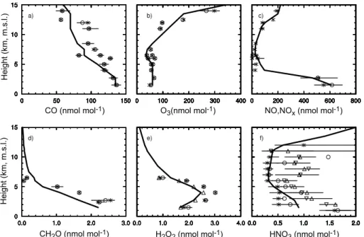
of the meteorological data were obtained from sonde and aircraft data (Skamarock et al., 2000). To start the convection quickly so that the intercomparison could focus on chemical species transport, the convection was initiated with 3 warm bubbles (3◦C perturbation) oriented in a NW to SE line. Simulations were integrated for a 3-h period. The initial profiles (Fig. 1) of the chemical species are primarily from the aircraft

5

observations obtained outside of cloud. CO is a surface tracer with a surface mix-ing ratio of 135 nmol mol−1. CO mixing ratios in the free troposphere range from 90–110 nmol mol−1 in the mid-troposphere and 50–90 nmol mol−1 in the upper tropo-sphere. O3 mixing ratios are fairly constant with height to about 7 km mean sea level (m.s.l.), above which O₃mixing ratios rapidly increase into the stratosphere. The initial

10

profile of NO_x is based on NO measurements outside of cloud. NO_x mixing ratios are ∼500 pmol mol−1 near the surface, but quickly decrease to values near 50 pmol mol−1 in the mid troposphere. At high altitudes NOx increases to 200 pmol mol−1. CH2O and H₂O₂ initial mixing ratios are from the low-flying aircraft that are combined with values obtained from the literature for high altitudes. CH2O decreases from the surface to

15

<200 pmol mol−1 in the mid-troposphere. H2O2mixing ratios peak near the top of the boundary layer then rapidly decrease in the mid to upper troposphere. HNO₃mixing ra-tios are based on NO_y measurements from the NASA SUCCESS (Jaegl ´e et al., 1998) and the NSF ELCHEM (Ridley et al., 1994) field campaigns.

3 Description of the models used in the intercomparison 20

Eight modeling groups submitted results for comparison. Tables 1 and 2 identify each group and key characteristics of their models. Details of model characteristics are discussed here.

(8)

ACPD

Full Screen / Esc

EGU

3.1 WRF with aqueous chemistry (WRF-AqChem, Mary Barth and Si-Wan Kim) A simple gas and aqueous chemistry scheme has been incorporated into the Weather Research and Forecasting (WRF) model (Barth et al., 2007). The WRF model solves the conservative (flux-form), nonhydrostatic compressible equations using a split-explicit time-integration method based on a 3rd order Runge-Kutta scheme

(Ska-5

marock et al., 2005; Wicker and Skamarock, 2002). Scalar transport is integrated with the Runge-Kutta scheme using 5th order (horizontal) and 3rd order (vertical) upwind-biased advection operators. Transported scalars include water vapor, cloud water, rain, cloud ice, snow, graupel (or hail), and chemical species.

The cloud microphysics is described by the single moment (bulk water) approach

10

(Lin et al., 1983). Mass mixing ratios of cloud water, rain, ice, snow, and hail are predicted. Cloud water and ice are monodispersed and rain, snow, and hail have prescribed inverse exponential size distributions. For the simulations performed here, hail hydrometeor characteristics (ρh = 900 kg m−3, No= 4×10

4

m−4) are used.

The gas-phase and aqueous chemistry (Barth et al., 2007) represent daytime

chem-15

istry of 15 chemical species, methane (CH₄), CO, O₃, hydroxyl radical (OH), hydroper-oxy radical (HO2), methylhydroperoxy radical (CH3OO), NO2, NO, HNO3, H2O2, methyl hydrogen peroxide (CH3OOH), CH2O, formic acid (HCOOH), sulfur dioxide (SO2), aerosol sulfate (SO₄), and ammonia (NH₃). Dissolution of soluble species is assumed to be in Henry’s Law equilibrium for low solubility species (e.g. CO) or is treated as

20

diffusion-limited mass transfer for high solubility species (Barth et al., 2001). When cloud water or rain freezes, the dissolved species is retained in the frozen hydrome-teor. Adsorption of gases onto ice or snow was not included in the simulation. The acidity of the cloud water and rain drops are calculated separately based on a charge balance. The chemical mechanism is solved with an Euler backward iterative

approxi-25

mation using a Gauss-Seidel method with variable iterations. A convergence criterion of 0.01% is used for all the species.

(9)

ACPD

Full Screen / Esc

EGU

(see Sect. 3.3) which follows DeCaria et al. (2005). The parameterization uses ob-served National Lightning Detection Network (NLDN) and lightning interferometer data to determine when a lightning flash occurs and whether that flash is a cloud-to-ground (CG) stroke or an intracloud (IC) stroke. Lightning NO is distributed vertically either as a Gaussian distribution peaking in the mid-troposphere (CG flashes) or as a bimodal

5

distribution peaking in the upper troposphere and mid-troposphere (IC flashes). At each model level, NO is divided equally among all grid cells within the 20 dBZ region of the storm.

The model is configured to a 160×160×20 km3 domain with 161 grid points in each horizontal direction (1 km resolution) and 51 grid points in the vertical direction with a

10

variable resolution beginning at 50 m at the surface and stretching to 1200 m at the top of the domain. The simulation was integrated at a 10 s time step. To keep the convec-tion near the center of the model domain, the grid is moved at 1.5 m s−1eastward and 5.5 m s−1_southward.

3.2 Chien Wang’s convective cloud model with chemistry (C. Wang)

15

The convective cloud model of Wang and Chang (1993a) coupled with chemistry solves the 3-D pseudo-elastic form of the continuity equation. The thermodynamic equations use an ice-liquid potential temperature as a conserved variable (Tripoli and Cotton, 1981). A δ four-stream radiation code Fu and Liou (1993), with predicted O3, water vapor, and liquid and ice phase hydrometeors, is used to compute the radiation transfer

20

at both short and long waves (Wang and Prinn, 2000). The advection of the chemical species including aerosols is calculated by using a revised Bott scheme (Bott, 1989, 1993) by Wang and Chang (1993a).

The cloud microphysics module predicts both number concentration and mass mix-ing ratios of cloud particles (e.g., a 2-moment scheme; Wang and Chang, 1993a). Two

25

liquid and two ice phase hydrometeors are represented in the model version for this in-tercomparison. The precipitating ice hydrometeor has graupel-like characteristics. The aerosol module used for the current simulations has a prognostic CCN (hygroscopic)

(10)

ACPD

Full Screen / Esc

EGU

and IN (insoluble) calculation (Wang and Prinn, 2000). The CCN and IN calculations include transport, nucleation, and precipitation scavenging. The initial surface number concentration of CCN and IN is set to be 500 cm−3and 100 L−1, respectively. Note that the actual nucleation rate of aerosols is determined by both the availability of aerosols and temperature as well as supersaturation at the grid point (Wang, 2005a).

5

The chemistry sub-model predicts atmospheric concentrations of 25 gaseous and 8 aqueous chemical species (in both cloud droplets and raindrops and thus 16 prognostic variables), undergoing more than 100 reactions of NOx-HOx-O3-CO-CH4-Sulfur chem-istry as well as transport and microphysical conversions (Wang and Chang, 1993a; Wang et al., 1998a; Wang and Prinn, 2000). Dissolution of soluble species is

param-10

eterized via diffusion-limited mass transfer. When freezing of liquid hydrometeors oc-curs, the dissolved gases are assumed to be retained in the frozen hydrometeors. The chemistry mechanism is solved with the Livermore solver for ordinary differential equa-tions (LSODE) (Hindmarsh, 1983; Wang et al., 1998a). A module of heterogeneous uptake by ice particles of several key chemical species including O3, H2O2, HNO3,

15

CH2O, CH3OOH, SO2, and H2SO4 based on the first-order reaction approximation is also included (Wang, 2005b).

The production of NOx from lightning follows the disk model of Wang and Prinn (2000). The lightning rate is derived as a parameterization of actually predicted collision rate between ice crystals and graupel as well as dynamic variables by the model. A

20

prescribed CG/IC ratio (not predicted by the parameterization) of 5% is adopted based on the observation. NO production is set to be 465 moles NO per flash for both IC and CG flash. The freshly-produced NO molecules are distributed vertically based on either two (IC) normal distributions centered respectively at ice crystal and graupel concentrated layers or one (CG) such distribution centered at the latter layer, generally

25

following DeCaria et al. (2000).

The model domain is 145×120 km2 horizontally with a 1 km spatial resolution. The model domain extends from the surface to 20 km with a uniform grid spacing of 400 m. The time step for the 3 h integration is 3 s.

(11)

ACPD

Full Screen / Esc

EGU

3.3 UMd/GCE (K. Pickering, L. Ott, G. Stenchikov)

The UMd/GCE modeling system consists of the 3-D Goddard Cumulus Ensemble (GCE) model (Tao and Simpson, 1993; Tao et al., 2001) and the University of Mary-land offline cloud-scale chemical transport model (CSCTM; DeCaria et al., 2005). The output of the GCE model is used to drive the CSCTM.

5

The GCE model hydrodynamics is based on a complete set of compressible, nonhy-drostatic equations in a Cartesian coordinate system. A second order finitedifference scheme in the vertical direction and the positive definite non-oscillatory horizontal ad-vection scheme with small implicit diffusion (Smolarkiewicz, 1984; Smolarkiewicz and Grabowski, 1990) are employed. Open boundary conditions of Klemp and Wilhelmson

10

(1978b) are used at the lateral boundaries. Newtonian damping is applied to the po-tential temperature and components of horizontal velocity at the top of the domain at about 25 km. A parameterization of sub-grid turbulent mixing is based on the prog-nostic equation for turbulent kinetic energy (Deardorf, 1975; Klemp and Wilhelmson, 1978a, b; Soong and Ogura, 1980). Turbulent mixing is handled in the cloud model

15

using a turbulent diffusion approximation.

To parameterize cloud microphysics a Kessler-type scheme (Kessler, 1969; Houze, 1993) for liquid hydrometeors (cloud water and rain) and the three-category scheme of Lin et al. (1983) for solid hydrometeors (ice, snow, and hail) are employed. The hydrometeors are assumed to be spherical with exponential size distributions except

20

for cloud water and cloud ice, which are monodisperse. Hail characteristics are used for the simulation.

Output from the 3-D GCE model simulation was used to drive a 3-D Cloud-Scale Chemical Transport Model (CSCTM, DeCaria et al., 2005). Temperature, density, wind, hydrometeor (rain, snow, graupel/hail, cloud water, and cloud ice), and diffusion

coeffi-25

cient fields from the GCE model simulation are read into the CSCTM every ten minutes, and these fields are then interpolated to the model time step of 15 s. The transport of chemical species is calculated using a van Leer advection scheme (Allen et al., 1991).

(12)

ACPD

Full Screen / Esc

EGU

The lightning NO scheme in the CSCTM, described fully in DeCaria et al. (2005), is based on observed flash rate data. CG flash rates were calculated from NLDN ob-servations and IC flash rates were determined by subtracting CG flash rates from total lightning flash rates obtained from interferometer observations. NO from CG flashes is distributed according to a Gaussian distribution peaking in the mid-troposphere while

5

NO from IC flashes is distributed bimodally based on the typical vertical distributions of the VHF sources of IC and CG flashes from MacGorman and Rust (1998). NO from both types of flashes is also distributed vertically proportional to pressure. In each model layer, lightning NO is horizontally distributed uniformly to all grid cells with computed radar reflectivity greater than 20 dBZ. Production per CG flash (PCG) was

10

estimated to be 390 mol NO per flash based on the mean peak current of CG flashes observed by the NLDN and a relationship between peak current and energy dissipated (Price et al., 1997). An estimate of NO production per IC flash (PIC) was obtained by assuming various PIC/PCG ratios and comparing the results with anvil aircraft mea-surements. Assuming a PIC/PCG ratio of 0.5 produced a favorable comparison with

15

observed in cloud NOx mixing ratios and as a result, PIC was estimated to be 195 moles NO per flash.

The CSCTM combines transport and lightning production with a chemical solver (SMVGEAR-II, Jacobson, 1995) and photochemical mechanism to simulate the chem-ical environment within the storm. The reaction scheme focuses on ozone

photochem-20

istry, containing the nonmethane hydrocarbons ethane, ethene, propane, and butane as described in DeCaria et al. (2000, 2005). The chemical scheme involves 35 ac-tive chemical species, 76 gas phase chemical reactions, and 18 photolytic reactions. Soluble species are removed from the gas phase by cloud and rain water with a depen-dence on Henry’s Law coefficients. Uptake by ice is not included. Aqueous and

multi-25

phase reactions are not included. Photolysis rates are calculated as a function of time and are perturbed by the cloud, using typical summertime estimates from Madronich (1987) and cloud thickness taken from the GCE model output. Initial condition profiles of PAN, ethane, ethene, propane, and butane were taken from profiles constructed

(13)

ACPD

Full Screen / Esc

EGU

using observations from the 12 July STERAO storm by DeCaria et al. (2005). The single column “spin-up” version of the CSCTM was run for 15 min to allow the chemical concentrations to come into equilibrium before starting the simulation of the storm.

The UMd/GCE modeling system was integrated in a domain of 360×328×25 km3 in the x, y and z directions, respectively. The horizontal grid spacing was 2 km in

5

both horizontal directions, and 0.5 km in the vertical. The GCE meteorology model was integrated using a 3 s time step to maintain numerically stability. The chemistry transport model is updated with a 30 s time step (though SMVGEAR-II itself uses a smaller time step based on stiffness).

3.4 RAMS (M. Leriche and S. Cautenet)

10

Gas and aqueous chemistry have been incorporated into the RAMS version 4.3 (Cotton et al., 2003). The basic equations in RAMS for solving the dynamical and thermody-namical variables are non-hydrostatic time-split compressible. The available options in the model include resolution ranging from few meters to a hundred kilometers, do-mains from a few kilometers to the entire globe and a suite of physical options for

tur-15

bulence closure, cloud microphysics, radiation, lower boundary (soil/vegetation/snow and ocean surface), upper and lateral boundary conditions. RAMS has a multiple grid nesting scheme leading to solve the model equations simultaneously on any number of meshes.

The cloud microphysics module predicts both number concentration and mass

mix-20

ing ratios of cloud particles, i.e. a two-moment bulk scheme (Meyers et al., 1997), using gamma distributions to represent the hydrometeor size distributions. For the simula-tion performed here, the water categories include cloud and rain drops and three ice condensate species: pristine ice, snow, and hail.

The chemistry module includes both gas and aqueous phase chemistry. For

gas-25

phase chemistry, the mechanism includes 29 species and describes the reactivity of ozone, NO_y and VOC including isoprene chemistry (Arteta et al., 2006; Taghavi et al., 2004). For aqueous-phase chemistry, the mechanism includes 10 species and

(14)

ACPD

Full Screen / Esc

EGU

represents the HO_x chemistry and the formation of nitrate, sulfate and formic acid (Audiffren et al., 2004). For the exchange of chemical species between gas phase and liquid hydrometeors, the mass transfer kinetic formulation of Schwartz (1986) is used taking into account the possible deviation from Henry’s law equilibrium. The redistribution of chemical species by microphysical processes is only considered for

5

liquid hydrometeors. Therefore, when freezing of liquid water occurs, the dissolved species are degassed. The interactions of chemical species with ice phase are not yet implemented in the model.

The lightning-NOxparameterization is based on Pickering et al. (1998). The parame-terization consists of four parts: flash rate, flash type, flash location and NO production

10

rate. The flash rate is computed from the maximum vertical velocity using a power law. The fractions of intracloud (IC) and cloud to ground (CG) flash are computed by estimating the depth of the layer from the freezing level (the 0◦C isotherm in the cloud) to the cloud top. The CG flashes are placed within the 20 dBZ region from the surface to the model-calculated –15◦C isotherm and the IC flashes in the region of the cloud

15

above the –15◦C isotherm. The NO production rate is then calculated for each CG and IC flash using different rate values for CG and IC flashes.

For the simulation of the STERAO storm, two nesting grids are used, the large one of 240×240×20 km3 with a horizontal resolution of 3 km and the small one of 120×120×20 km3 with a horizontal resolution of 1 km. The small grid moves into the

20

large one with a constant velocity of 1.5 m s−1 towards the east and 5.5 m s−1 south-ward. A 5 s time step is used.

3.5 Meso-NH (J.-P. Pinty, C. Barthe, and C. Mari)

The Meso-NH model integrates an anelastic system of equations. The model can be used to simulate real cases (starting from ECMWF analyses) or ideal cases (the

25

STERAO case for instance). The model is fully explicit. It contains all the necessary parameterizations to run a meteorological case. Grid nesting is available with 1 or 2-way coupling. In addition, the model contains a flexible chemical scheme, an aerosol

(15)

ACPD

Full Screen / Esc

EGU

scheme, a 1- or 2-moment microphysical scheme and an electrical scheme.

The Multidimensional Positive Definite Advection Transport Algorithm (MPDATA) is used for the advection scheme, and turbulence is parameterized with a 3-D scheme. In addition, a gravity wave damping layer is placed between the model top and 15 km height.

5

The cloud microphysics is described by a mixed-phase scheme (Pinty and Jabouille, 1998) that takes into account 6 water variables (water vapor, cloud droplets, raindrops, pristine ice, snow and graupel). For this study, graupel-like characteristics are used. Only mass mixing ratios of these microphysical species are predicted. Meso-NH also contains an explicit electrification and lightning flash scheme (Barthe et al., 2005).

10

The electric charges are carried by each of the hydrometeor categories and are sep-arated via non-inductive processes (i.e., ice-graupel collisions). Lightning flashes are triggered when the ambient electric field exceeds a threshold (167ρ(z) kV m−1). The lightning flashes produce both bi-directional leaders and branch streamers (Barthe et al., 2005). Nitrogen oxides are added along the lightning flash path as a function of the

15

pressure and the channel length as suggested by Wang et al. (1998b) from laboratory experiments (Barthe et al., 2007).

For these simulations, only the scavenging of the soluble gases, CH2O, H2O2, and HNO3 are considered. The partitioning between gas and liquid phases is calculated following the mass transfer kinetic formalism of Schwartz (1986). These species do not

20

react chemically. The scavenged gases are tracked in the cloud droplets and in the rain drops only, but not in the ice phase. Note that the liquid drops do get transported to the glaciated regions of the modeled storm. CO and O3are insoluble. NOx is represented by 2 variables: the first one corresponds to the background NO_x and the second one includes both background and the NOxproduced from lightning.

25

The simulation is configured to that described by Skamarock et al. (2000). The computational domain is 160×160×50 grid points with a horizontal resolution of 1 km and a vertical spacing ranging from 75 m at the ground to 700 m in the stratosphere. The time step (2 s) is low to get an accurate transport of the trace gases.

(16)

ACPD

Full Screen / Esc

EGU

3.6 SDMST (John Helsdon, Richard Farley)

The 3D SEM (Storm Electrification Model) has fully coupled microphysical, electrical and chemical processes. The model is a modified form of the 3-D nested grid model developed by Terry Clark and associates (Clark, 1977; Clark, 1979; Clark and Farley, 1984; Clark and Hall, 1991). The model is nonhydrostatic and uses the anelastic

ap-5

proximation to eliminate sound waves. For the dynamics, the model employs the flux form of the second-order operators of Arakawa (1966) for the spatial derivatives, and treats time derivatives using a second-order leapfrog scheme. This formulation allows the model to conserve kinetic energy. Advection of scalar quantities uses the mul-tidimensional positive-definite advection transport algorithm (MPDATA) developed by

10

Smolarkiewicz (1984) and Smolarkiewicz and Clark (1986). Subgrid-scale turbulence is parameterized according to first-order theory.

The model employs the single moment (mixing ratio) microphysical parameterization scheme of Lin et al. (1983) which allows five hydrometeor classes; cloud water, rain, cloud ice, snow, and graupel/hail. For the simulation reported here, the model uses

15

parameters characteristic of hail to represent the graupel/hail field. The treatment of electrical processes follows Helsdon and Farley (1987) and Helsdon et al. (2001). Each hydrometeor class has an associated charge density in addition to the positive and neg-ative small ion concentrations that combine to form the total charge density, which is related to the electrical potential through Poisson’s equation. Gas phase chemical

pro-20

cesses are included in the model as described in Zhang et al. (2003). This formulation allows 18 reactions involving nine tracked chemical species which include NO, NO₂, O3, CH4, CO, OH and HO2, with HNO3as a sink.

The simulation includes an explicit prediction of intracloud lightning discharges as described in Helsdon et al. (1992) and Helsdon et al. (2002). A lightning channel is

25

initiated when and where a threshold electric field is attained (225 kV m−1 in this case) and propagates bi-directionally away from the initiation point following the electric field vector. The channel terminates when the electric field at the ends of the propagating

(17)

ACPD

Full Screen / Esc

EGU

channel drops below a preset value (75 kV m−1). Once the channel is formed, its linear charge density is calculated from theory and converted into an equivalent small ion density. The charged channel modifies the electric field and consequently modifies the electric energy in the domain in a physically consistent manner. By calculating the elec-trical energy just before and immediately after the discharge, the energy dissipation can

5

be determined. NO production (9×1016NO molecules J−1 _{at sea level) is proportional} to this electrical energy change and pressure, and is limited to the immediate vicinity of the lightning channel.

The simulation is configured to a 120×120×20 km3 domain using 1 km horizontal grid spacing and 250 m vertical resolution. The model integrations employed a 2-s

10

time step. A Galilean transformation is applied to keep the main convection within the interior regions of the domain. For the 10 July STERAO case the grid translates to the east at 4 m s−1and to the south at 5 m s−1.

3.7 DHARMA (A. Fridlind, A. Ackerman)

The DHARMA (Distributed Hydrodynamic Aerosol-Radiation-Microphysics Application)

15

model treats atmospheric and cloud dynamics with a large-eddy simulation code (Stevens and Bretherton, 1996) that solves an anelastic approximation of the Navier-Stokes equations appropriate for deep convection (Lipps and Hemler, 1986).

Embedded within the dynamics code, DHARMA treats aerosol and cloud micro-physics with the CARMA (Community Aerosol-Radiation Model for Atmospheres) code

20

(Ackerman et al., 1995; Jensen et al., 1998). Aerosols, water drops, ice crystals, and solute within the drops and crystals are tracked in a range of sizes (16 size categories each). The density of ice is a function of size, roughly representative of conical graupel. Microphysical processes include aerosol activation into drops, condensational growth and evaporation of drops, gravitational collection, spontaneous and collision-induced

25

drop breakup, homogeneous and heterogeneous freezing of aerosols and drops, de-positional growth and sublimation of ice, sedimentation of liquid and ice, melting, and

(18)

ACPD

Full Screen / Esc

EGU

Hallett-Mossop rime splintering. The microphysics treatment is identical to that used by Fridlind et al. (2005), where further detail is provided.

The DHARMA model only transports trace gases. Chemistry and production of NOx from lightning are not included in the model.

Results shown here are for uniform 1 km horizontal resolution and 250 m vertical

5

resolution over a 120×120×20 km3 domain, which is nudged to the initial profile along each face. Dynamics and gravitational collection are advanced with a 5-s time step; all other microphysical processes are advanced with a time step of 0.2 to 5 s that is chosen based on the processes that are active in each grid cell as the simulation progresses. 3.8 Vlado Spiridonov’s convective cloud model with chemistry (Vlado Spiridonov,

10

Bosko Telenta)

The model (Spiridonov and Curic, 2003, 2005) is a three-dimensional, non-hydrostatic, time-dependant, compressible system using the dynamic and thermody-namics schemes from Klemp and Wilhelmson (1978a) and the bulk cloud microphysics scheme from Lin et al. (1983) that takes into account 6 water variables (water vapor,

15

cloud droplets, ice crystals, rain, snow, and graupel). The graupel hydrometeor class is represented as hail with a density of 0.9 g cm−3. The chemistry module includes sulfate chemistry (Taylor, 1989) both inside and outside clouds. The absorption of chemical species from the gas phase into cloud water and rainwater is determined by either Henry’s law equilibrium (Taylor, 1989), or by diffusion-limited mass transfer between

20

gas and liquid phases to include possible non-equilibrium states, (Barth et al., 2001). All equilibrium constants and oxidation reactions are temperature dependent according to the van’t-Hoff relation (Seinfeld, 1986). Cloud water and rainwater pH is calculated using the charge balance equation from Taylor (1989). The model includes a freez-ing transport mechanism of chemical species based on Rutledge et al. (1986). Thus,

25

when water from one hydrometeor class is transferred to another, the dissolved scalar is transferred to the destination hydrometeor in proportion to the water mass that was transferred. Production of NO from lightning is not parameterized in the Spiridonov

(19)

ACPD

Full Screen / Esc

EGU

model.

For the intercomparison simulation, the model is configured to a domain of 140×140×15 km3with 1 km horizontal resolution and 500 m vertical resolution. A 10 s time step is used for the integration.

4 Results

5

Four types of model results are presented. First, the storm intensity and structure are analyzed by intercomparison of peak vertical velocity and radar reflectivity with obser-vations. Second, the redistribution of CO, O₃and NO_x are presented, and anvil mixing ratios are compared with analyzed UND Citation aircraft measurements. Then the flux of air, CO and NOx through a plane across the anvil is compared to that determined

10

from the observations. Lastly the mixing ratios of CH₂O, H₂O₂, and HNO₃ in the anvil are compared among models.

4.1 Storm intensity and structure

The maximum vertical velocity in the model domain was recorded at 10-minute in-tervals (Fig. 2). Each model shows a rapid increase in peak updraft velocity at the

15

beginning of the simulation. Most simulations maintain peak updrafts above 24 m s−1 during the remainder of the simulation, while radar observations show peak updrafts to be between 24 and 38 m s−1_{. Transitions to updraft velocities of 35 m s}−1 _{or more are} seen by C. Wang’s model, WRF-Aqchem, DHARMA, and Meso-NH. The height of the peak updraft ranges from 7 km to 14 km m.s.l., which is similar but somewhat higher

20

than observations.

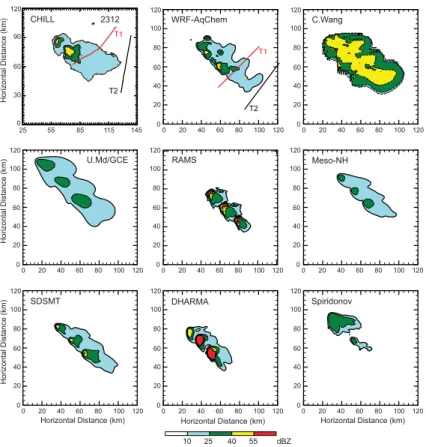
The storm structure can be evaluated by comparing the modeled radar reflectivity to the observed radar reflectivity. Both horizontal and vertical cross-sections of radar reflectivity are examined. At 23:12 UTC 10 July, the CSU CHILL radar reflectivity at z = 10.5 km m.s.l. indicates two convective cores oriented in a northwest-southeast

(20)

ACPD

Full Screen / Esc

EGU

line with an anvil spreading to the east-southeast (Fig. 3). After 1 h of simulation, the results from the models have 2–3 convective cores oriented northwest-southeast. The magnitude of the reflectivity differs among models due to 1) whether graupel charac-teristics (C. Wang, Meso-NH, DHARMA models) or hail characcharac-teristics are modeled, 2) horizontal resolution, and 3) single-moment versus multi-moment (C. Wang, DHARMA,

5

RAMS models) microphysics parameterizations. The width of the anvil varies among models. The observed reflectivity has an anvil width of 32–40 km at 23:12 UTC, while model results range from 12.5 km to 45 km. Seifert and Weisman (2005) noted that double-moment microphysics parameterizations tend to produce broader anvils than single-moment microphysics parameterizations. The results from our study do not

dis-10

tinctly show this correlation. While C. Wang’s model with double-moment microphysics has a widespread anvil, DHARMA and RAMS have anvils similar in width to the mod-els with single-moment microphysics. Other factors contributing to the anvil width are the graupel or hail characteristics used (which influences the particle’s fall speed), the dynamics formulation, and the horizontal resolution.

15

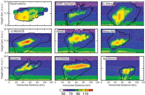
The vertical cross section of observed reflectivity along the storm axis (Fig. 4) shows that the northwest core (left side of figure) is decaying while the southeast core is reaching its mature stage. During the multicell stage of the storm, radar reflectivity plots show 2 to 4 convective cores being active at any given time. All of the models show 3 convective cores, with all cores of approximately the same reflectivity

magni-20

tude except for the Meso-NH model. The Meso-NH model has weaker reflectivity most likely because of the graupel (rather than hail) characteristics used in their microphysics parameterization. While the reflectivity in the observed anvil is weak (5–20 dBZ) and somewhat extensive (>35 km from the southeast core to the anvil edge), the simulated anvils are stronger (5–35 dBZ) and less extensive (15–25 km from the southeast core to

25

the anvil edge). The maximum height of the modeled reflectivity varies among models. The reflectivity simulated by Spiridonov only reaches 11.5 km m.s.l., while the reflec-tivity simulated by the C. Wang and RAMS models reach 16.5 km m.s.l. Observations show the reflectivity top to be 14.5 to 16.5 km m.s.l.

(21)

ACPD

Full Screen / Esc

EGU

In summary, the discrepancies among models for radar reflectivity, which are mainly due to the differences between the treatments of cloud microphysics, highlight the dif-ficulty of modeling the realistic structure of clouds even using cloud resolving models. Nevertheless, the modeled cloud structures are all reasonably simulated. Thus, it is possible to use these models to simulate trace gas transport as part of the

intercom-5

parison.

4.2 Distributions of CO, O₃, and NO_x

Mixing ratios of CO, O3, and NOxare compared to observations using two approaches. First, model results are evaluated with aircraft measurements which were obtained from the University of North Dakota (UND) Citation aircraft as it flew across the anvil.

10

Second, cross-sections of the mixing ratios are compared to a derived cross-section obtained from several transects of the anvil by the aircraft.

The UND Citation aircraft sampled the outflow region of the storm by performing across-anvil transects at different levels in the anvil (transects indicated in Fig. 3). Two transects are used to compare model results with observations. The first transect is

15

10 km downwind of the southeastern-most convective cell at 23:10 UTC (which corre-sponds to t = 1 h in the simulations) at 11.6 km m.s.l. The second transect is ∼50 km downwind of the southeastern-most convective cell at 23:35 UTC (corresponding to t = 1 h 30 min in the simulations) at 11.2 km m.s.l.

Mixing ratios of CO in the anvil are observed to be enhanced compared to the

back-20

ground upper troposphere (Fig. 5) because convective transport moves high mixing ratios from the boundary layer to the upper troposphere. Conversely, O3mixing ratios are lower in the anvil than in the upper troposphere because relatively-low O3 mixing ratios are transported from the boundary layer. The model simulations predict these enhancements and depletions of CO and O3 mixing ratios, which agree with the

ob-25

servations (Fig. 5), especially in the core of the anvil. All models underpredict the O3 mixing ratio on the southwest edge of the anvil, a feature that may be attributed to mix-ing of stratospheric air as is discussed below. Nevertheless, all the models do a good

(22)

ACPD

Full Screen / Esc

EGU

job transporting these passive tracers within the anvil.

Observed NO mixing ratios (Fig. 6) are strongly enhanced within the anvil compared to the background upper troposphere primarily due to lightning production of NO. Mod-eled NOx mixing ratios show the importance of the lightning source. The DHARMA and Spiridonov models do not include production of NO_x from lightning and therefore

5

substantially underpredict the NOx mixing ratios. The other models, which include lightning-produced NOx, generally show NOx mixing ratios elevated compared to the DHARMA and Spiridonov models within the anvil. For the first transect, WRF-AqChem, C. Wang, Meso-NH, and SDSMT NOx mixing ratios are similar to the observations, but for shorter across-anvil distances. Only the Meso-NH model has a similar area

10

under the curve as the observations, indicating the total amount of NO_x placed into the 11.8 km m.s.l. height is realistic (note that mass fluxes of NOx integrated over the across-anvil area and over time are discussed in the next section). For the second transect, all of the models that include NO_x production by lightning agree reasonably well with observations. This is the first time simulated lightning NOx production from a

15

specific model transect has been directly compared with observations from the corre-sponding specific aircraft transect of a storm anvil. To obtain NO_x mixing ratios similar in magnitude to observations is encouraging and indicates that model parameteriza-tions are capturing the key parameters of lightning NOxproduction.

Skamarock et al. (2003) analyzed the UND Citation aircraft data taken across the

20

anvil of the storm. The Citation aircraft mapped out the anvil structure during ∼1 h 30 min time period by traversing the anvil in horizontal passes, approximately perpen-dicular to the long axis of the anvil, at elevations starting at approximately 11.8 km m.s.l. (close to the anvil top) and ending at approximately 6.8 km m.s.l. Skamarock et al. (2003) projected the cloud particle concentration, CO, O3, and NO observations

25

onto a vertical plane using an objective analysis procedure. Model predictions of these variables taken along a similar plane (similar to the T2 cross-section shown for WRF-AqChem in Fig. 3) can then be compared to the analyzed observations.

(23)

ACPD

Full Screen / Esc

EGU

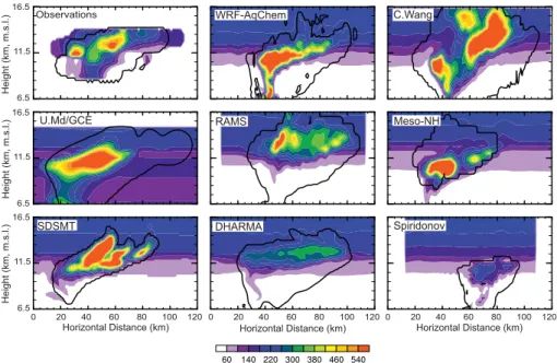
Fig. 7. The analyzed observations are for ice >25 µm diameter (Dice) based on the measurements from the Particle Measuring Systems 2-D probe (Dye et al., 2000). The results from the models tend to match or over-predict the observations. The results from the C. Wang and RAMS models are only for Dice>25 µm giving good agreement with observations. While the DHARMA results are also only for ice with D_ice >25 µm,

5

the results overpredict the ice particle number, suggesting other factors contribute to in-creased predicted ice particle number. Using graupel characteristics instead of hail can also increase ice concentrations in the anvil region because graupel has a smaller fall speed and therefore is carried further into the anvil. The models that predicted only the mass of the cloud particles (WRF-AqChem, UMd/GCE, Meso-NH, SDSMT, Spiridonov)

10

assumed a diameter for the ice hydrometeor category (for example, WRF-AqChem set Dice=45 µm) for the purposes of estimating the number concentration. The calculation of number concentration is very dependent on the assumed ice diameter since the anvil is primarily composed of small ice particles.

Carbon monoxide mixing ratios analyzed from the observations (Fig. 8) reach

15

110 nmol mol−1 or so in the anvil. Simulated CO mixing ratios also reach those val-ues in the anvil. There is a slight underprediction of CO seen in the WRF-AqChem model. In general, the models reasonably simulate CO mixing ratios in the anvil.

Vertical cross-sections of observed O3 (Fig. 9) show O3 being depleted in the anvil to values of about 80–100 nmol mol−1_{, but also show a small region of}

downward-20

intruding, high (>300 nmol mol−1) O3at the top of the anvil on the SSW edge (upper left part of figure). The C. Wang and RAMS models also show some downward intrusion of O₃ on the SSW upper edge of the anvil (note the change in vertical gradient of O₃ at z = 13.5 km m.s.l. on the left side of the anvil) or upward intrusion of low O3 at the top of the convective cores, but none of the other models reproduce the change in the

25

O₃ vertical gradient. Both the C. Wang and RAMS models have tall convective cores at t = 1 h (Fig. 4), thus the vertical extent of the updraft in connection with turbulent mixing at the tropopause may be responsible for the high O3 at the top of the anvil on the SSW edge. In agreement with observations, all the models show mixing ratios of

(24)

ACPD

Full Screen / Esc

EGU

80 nmol mol−1in the anvil.

The analyzed NO mixing ratios from observations have peaks of NO of over 500 pmol mol−1 _{(Fig. 10) within a broad region of NO >200 pmol mol}−1_{. Note that the} observations are of NO while the model results are of NOx. By assuming photochemi-cal equilibrium between NO and NO2, NOxmixing ratios are approximately 30% greater

5

than NO mixing ratios (Skamarock et al., 2003). Thus, modeled NO_xshould be ∼30% greater than the observed NO. Results from models that did not include production of NOx from lightning (DHARMA, Spiridonov) do not predict the NOx>500 pmol mol−1 peaks, but instead show NO_x∼200 pmol mol−1 in the anvil; much less than that ob-served. The models with production of NOx from lightning (WRF-AqChem, C. Wang,

10

UMd/GCE, RAMS, Meso-NH and SDSMT) do predict peaks of NOxon the same order of magnitude as the observations. These models also have a broad region of NO_x mixing ratios between 150 and 250 pmol mol−1_{, similar to those seen in the} observa-tions. To obtain the observed peak values of the NOx, production from lightning must be modeled.

15

4.3 Mass fluxes in the anvil outflow

Utilizing the modeled mixing ratio of (C) in the anvil cross-sections (shown in Figs. 8– 10) and the horizontal velocity (U⊥) perpendicular to the cross-section plane, estimates of mass fluxes can be made. Corresponding mass fluxes of air, CO, and NOx are derived from the aircraft measurements (Skamarock et al., 2003) for comparison to the

20

model results. The calculation of the modeled mass flux density is

flux = P anvil cells ρ U ⊥ C ∆ℓ ∆z P anvil cells ∆ℓ ∆z

where ∆ℓ and ∆z are the horizontal and vertical grid cell spacing within the anvil. The flux density is determined only in the region where cloud particles exist in the anvil.

(25)

ACPD

Full Screen / Esc

EGU

Table 3 lists the anvil area as well as the fluxes of air mass, CO, and NO_x aver-aged over a 1 h time period, which is comparable to the time period of the aircraft measurements. Each model’s average mass flux can be compared to the mass flux derived from observations, which was determined by Skamarock et al. (2003) from the analyzed cross section.

5

While the analyzed anvil area taken from the observations is 315 km2, the modeled anvil area ranges from 109 km2to 590 km2, which are within –65 and 90% of the ana-lyzed observed area. The air mass flux determined from the observations is 5.9 kg m−2 s−1, while that predicted by the models ranges from 6.6 to 9.1 kg m−2 s−1. Note that there is also some uncertainty in the observed anvil area and flux densities (Skamarock

10

et al., 2003) associated with uncertainties in the in situ measurements and in temporal changes in these measured species and in the anvil cross-section area as the mea-surements were taken. All of the models overpredict the air mass flux, suggesting that the modeled wind speeds in the anvil are too strong. The CO flux density calculation from the observational analysis is 1.9×10−5moles m−2s−1, while the modeled CO flux

15

densities range from 1.93 to 2.8×10−5moles m−2s−1. We find that 4 models are within 5% of the analyzed CO flux density and a total of 7 models are within 33%. However, because the air mass flux is over-predicted by these same models, a correction to the air mass flux density would result in CO flux densities being smaller than the analysis of the measurements. The NO_x flux density derived from the observations includes

20

NOxproduced from lightning and has a value of 5.8×10−8moles m−2s−1. The NOxflux densities determined from models without lightning-NOx production (DHARMA, Spiri-donov) are 4.3×10−8 and 2.7×10−8moles m−2s−1, while the models that do include lightning-NO_x production are between 3.9 and 13.0×10−8_{moles m}−2_s−1_{. We find that} the variability among the modeled NOxflux densities is clearly higher than that for the

25

(26)

ACPD

Full Screen / Esc

EGU

4.4 Distributions of CH₂O, H₂O₂, and HNO₃

Soluble and reactive chemical species, such as formaldehyde, hydrogen peroxide and nitric acid, are important to tropospheric ozone chemistry. In simulating CH₂O, H₂O₂, and HNO3, species with different solubility coefficients and different chemical reactiv-ity are represented. Because there were no observations of CH2O, H2O2, and HNO3

5

in the outflow region of the 10 July 1996 STERAO storm, comparisons to measure-ments are not possible. While other field campaigns have measured one or more of these species near convection, none of the campaigns have done a budget (detrained species in the anvil minus entrained species into the convective core) nor have the measurements been near the storm core as these model results are. These

previ-10

ous field campaigns have shown some enhancement of CH2O and H2O2 and strong depletion of gas-phase HNO₃ in convective outflow regions compared to their back-ground upper troposphere mixing ratios. Here, we compare gas-phase mixing ratios for these 3 species to find similarities and differences among model approaches. How the simulated results compare to past field campaigns is discussed at the end of the

15

section.

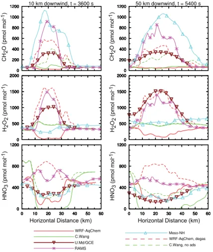
The soluble, reactive species are simulated by 5 models: WRF-AqChem, C. Wang, UMd/GCE, RAMS, and Meso-NH. Model results along the same two aircraft transects are used for the comparison (Fig. 11). In contrast to the CO and O₃ results, the modeled CH2O, H2O2, and HNO3 gas-phase mixing ratios vary significantly among

20

models. For CH2O, the Meso-NH, RAMS, and UMd/GCE simulations have enhanced CH₂O mixing ratios compared to their values in the background upper troposphere. The WRF-AqChem and C. Wang simulations have anvil mixing ratios that are depleted or similar to the background upper troposphere mixing ratios. One explanation for the disagreement among model results is the manner in which soluble species are treated

25

with the ice phase. The Meso-NH, RAMS, and UMd/GCE models do not include sol-uble species in the ice phase while WRF-AqChem and C. Wang models do. Both the WRF-AqChem and C. Wang models use a retention efficiency of 100% when cloud

(27)

ACPD

Full Screen / Esc

EGU

and rain drops freeze. Thus, in these two models the CH₂O in the snow and hail is precipitated with their parent hydrometeor, transferred to the rain via melting, and rained onto the ground (Barth et al., 2001, 2007). The WRF-AqChem, degas curves in Fig. 11 illustrate the effect of not including soluble species in the ice phase. A sec-ond explanation for differences in CH2O mixing ratios is the effect of chemistry. The

5

Meso-NH model does not include gas or aqueous chemistry, while WRF-AqChem, C. Wang and RAMS do include gas-phase and aqueous chemistry, and UMd/GCE in-cludes only gaseous chemistry. Previous studies (Leriche et al., 2007; Barth et al., 2007) showed that both gas-phase and aqueous chemistry (using a chemistry mech-anism without non-methane hydrocarbons) reduce CH₂O mixing ratios in the anvil.

10

Similarly the assumption of Henry’s law equilibrium for gas-aqueous species transfer (UMd/GCE) could reduce gas-phase concentrations. Simulations without the produc-tion of NO from lightning performed by both the WRF-AqChem and C. Wang models show negligible differences from those shown in Fig. 11 for anvil CH2O mixing ratios within 50 km of the storm core.

15

For H2O2, the UMd/GCE and RAMS model results have enhanced mixing ratios in the anvil compared to the background upper troposphere. The C. Wang and Meso-NH model results have similar mixing ratios between the anvil and background upper troposphere, while the WRF-AqChem model results have depleted H2O2mixing ratios compared to the background upper troposphere. The effect of the ice phase

(WRF-20

AqChem, degas curve) would enhance H2O2 mixing ratios in the anvil substantially. Lightning production of NO does not affect the results shown by the WRF-AqChem and C. Wang models. The inclusion of aqueous chemistry does reduce anvil mixing ratios of H2O2 somewhat (Leriche et al., 2007; Barth et al., 2007). Furthermore, the treatment of the gas-aqueous species transfer could affect results, with the

assump-25

tion of Henry’s law likely reducing gas-phase mixing ratios. Modified photolysis rates may increase H2O2mixing ratios. The C. Wang and UMd/GCE models include cloud-modified photolysis reaction rates, while the other models do not. However, Barth et al. (2002) showed a very small effect of cloud-modified photolysis rates on H2O2mixing

(28)

ACPD

Full Screen / Esc

EGU

ratios in marine boundary layer clouds.

For HNO₃, all the models except the RAMS model has anvil mixing ratios that are depleted compared to the background upper troposphere. The C. Wang HNO3 gas-phase mixing ratios go to zero in the anvil, while other models show values between 200 and 300 pmol mol−1_{. The discrepancy is explained by adsorption of gas-phase}

5

HNO3onto ice and snow crystals which is included in the C. Wang model. When this process is not included (C. Wang, no ads curve), the HNO3mixing ratios in the anvil are similar to those predicted by the other models.

For soluble species, such as CH2O, H2O2, and HNO3, many processes affect their fate. Scavenging of these gases by the drops and ice tends to reduce their gas-phase

10

mixing ratios in the anvil. Aqueous chemistry also tends to reduce mixing ratios of CH2O and H2O2. Inclusion of dissolved species in the ice phase substantially reduces the gas-phase mixing ratios of CH2O, H2O2, and HNO3, but this is an uncertain re-sult because of the uncertainties and lack of knowledge concerning the physical and chemical processes occurring when cloud and rain drops freeze. Production of NO

15

by lightning does not affect the gas-phase mixing ratios of these species within 50 km of the storm core. Their mixing ratios may be affected further downwind as chemical aging occurs.

While measurements of formaldehyde, hydrogen peroxide, and nitric acid were not taken in the convective outflow of the 10 July 1996 STERAO storm, some of these

20

species have been measured during other field campaigns near convection. Stick-ler et al. (2006) found enhanced upper troposphere CH2O mixing ratios over Europe on a day influenced by convection compared to a day representative of background conditions. These measurements were taken well downwind of the convection there-fore allowing chemical aging (i.e. production of CH2O) to occur in the convective

out-25

flow plume. H2O2measurements reported for tropical oceanic convection sampled in PEM Tropics A (Cohan et al., 1999) showed that H₂O₂ convective outflow mixing ra-tios were moderately enhanced (330±140 pmol mol−1) compared to the unperturbed upper troposphere (200±110 pmol mol−1). These results support the C. Wang results

(29)

ACPD

Full Screen / Esc

EGU

(Fig. 11), but it must be recognized that the Cohan et al. measurements sampled trop-ical, oceanic convection (characterized by more liquid water and less ice) compared to the midlatitude, continental convection simulated in this study. Measurements of HNO3 (Popp et al., 2004) revealed large depletions of gaseous HNO₃ in cirrus sampled dur-ing the CRYSTAL-FACE experiment in Florida. Their measurements are in agreement

5

with the models showing gas-phase HNO3depleted mixing ratios (Fig. 11).

5 Conclusions

The intercomparison of convective scale cloud chemistry models simulating constituent transport in deep convection is the first of its kind. Simulations were performed based on the same initial conditions and similar model domain configurations. All eight

mod-10

els that participated in the intercomparison have reproduced the observed multicellular convection with radar reflectivity reaching >50 dBZ. Comparisons of carbon monoxide and ozone, which are primarily transported in convection, showed good agreement among models and with observations especially within the anvil. The models that included lightning production of nitric oxide predicted NOxmixing ratios of similar

mag-15

nitude to observed NO mixing ratios indicating that NO production from lightning is a key process to include for understanding the composition of convective outflow re-gions. Furthermore, the relatively good agreement with observations show that current cloud-scale parameterizations of lightning production of NO seem to be capturing the key parameters of this process. This is an important point because the

parameteriza-20

tions used ranged from physically-based NO production utilizing the explicit prediction of charge, to parameterizations based on peak updraft velocities, to those based on observed lightning flash input data.

Calculations of the anvil fluxes of air, CO and NOx are compared between models and analyzed observations. The models consistently overestimate the flux density of

25

air compared to the observed value, but flux densities of CO agree quite well with the observed value. The deviation among the models is 20% and less for the air and CO

(30)

ACPD

Full Screen / Esc

EGU

flux densities. Predicted NO_x flux densities are significantly more variable and tend to be greater than that estimated from observations.

Formaldehyde, hydrogen peroxide, and nitric acid, species that are soluble and chemically reactive, are compared just among the different models because obser-vations of these species were not made in the anvil region of the STERAO storm. For

5

all 3 species, the models produced very different results indicating the need for mea-surements of these species in the anvil region to better understand their convective processing. Potential reasons for the discrepancies among the models include the role of the ice phase, the impact of cloud-modified photolysis rates on these species mixing ratios, and representation of their chemical reactivity.

10

To improve parameterizations of convective transport of constituents in large-scale models, we can use these models to obtain general characteristics (e.g. vertical mass fluxes and wet deposition rates) of chemical constituent transport in a variety of con-vection types. Further research needs to be conducted to understand what processes control the fate of the soluble species formaldehyde, hydrogen peroxide, and nitric acid.

15

As part of this, measurements of these soluble, reactive species must concurrently be taken in both the inflow and outflow regions of a variety of convective storms.

Acknowledgements. The discussions and contributions of initial conditions and analyzed

observations from W. Skamarock are greatly appreciated. More information on the

in-tercomparison can be found at http://box.mmm.ucar.edu/people/barth/files/Chem Convec

20

Intercomparison/tracertransportdeepconvection.html. Wiebke Deierling is thanked for providing the radar-derived maximum updraft speeds and heights. The University of Maryland/Rutgers investigators thank W.-K. Tao for use of the Goddard Cumulus Ensemble Model to drive the cloud chemistry calculations. The National Center for Atmospheric Research is operated by the University Corporation for Atmospheric Research under the sponsorship of the National 25