Errors due to random noise in velocity measurement using incoherent-scatter radar

(1)

HAL Id: hal-00316282

https://hal.archives-ouvertes.fr/hal-00316282

Submitted on 1 Jan 1996

HAL is a multi-disciplinary open access

archive for the deposit and dissemination of sci-entific research documents, whether they are pub-lished or not. The documents may come from teaching and research institutions in France or abroad, or from public or private research centers.

L’archive ouverte pluridisciplinaire HAL, est destinée au dépôt et à la diffusion de documents scientifiques de niveau recherche, publiés ou non, émanant des établissements d’enseignement et de recherche français ou étrangers, des laboratoires publics ou privés.

Errors due to random noise in velocity measurement

using incoherent-scatter radar

P. J. S. Williams, A. Etemadi, I. W. Mccrea, H. Todd

To cite this version:

P. J. S. Williams, A. Etemadi, I. W. Mccrea, H. Todd. Errors due to random noise in velocity measurement using incoherent-scatter radar. Annales Geophysicae, European Geosciences Union, 1996, 14 (12), pp.1480-1486. �hal-00316282�

(2)

Ann. Geophysicae 14, 1480—1486 (1996) ( EGS — Springer-Verlag 1996

Errors due to random noise in velocity measurement

using incoherent-scatter radar

P. J. S. Williams1, A. Etemadi2, I. W. McCrea3, H. Todd4

1 Adran Ffiseg, Prifysgol Cymru Aberystwyth, SY23 3BZ, Wales 2 Blackett Laboratory, Imperial College, London SW1, England

3 Rutherford Appleton Laboratory, Chilton, Didcot OX11 0QX, England 4 University of Fiji, Fiji

Received: 24 January 1996/Revised: 19 August 1996/Accepted: 20 August 1996

Abstract. The random-noise errors involved in measuring the Doppler shift of an ‘incoherent-scatter’ spectrum are predicted theoretically for all values of ¹e/¹i from 1.0 to 3.0. After correction has been made for the effects of convolution during transmission and reception and the additional errors introduced by subtracting the average of the background gates, the rms errors can be expressed by a simple semi-empirical formula. The observed errors are determined from a comparison of simultaneous EISCAT measurements using an identical pulse code on several adjacent frequencies. The plot of observed versus pre-dicted error has a slope of 0.991 and a correlation coeffic-ient of 99.3%. The prediction also agrees well with the mean of the error distribution reported by the standard EISCAT analysis programme.

1 Introduction

The analysis of incoherent-scatter data is usually accom-plished by fitting a theoretical autocorrelation function (ACF) to the observed ACF. The noise errors in the derived ionospheric parameters are then estimated from the variance of the measurement at different lags of the ACF. A fundamental study of this analysis procedure has been made by Lehtinen (1986), who developed a full Bayesian theory of the inversion of incoherent-scatter ACFs, and by Vallinkoski (1988, 1989), who used this theory to estimate the statistical errors in multi-parameter fits. Vallinkoski demonstrated that in this analysis there was a minimum lag resolution below which there were no further improvements in the error level. This approach is the basis of the GUISDAP programmes which have been widely adopted for the optimum analysis of incoherent-scatter data. In a recent paper (Huuskonen and Lehtinen,

Correspondence to: P. J. S. Williams

1996) the authors have studied the accuracy of incoherent-scatter measurements for high signal levels and empha-sised the effect of significant correlation between different lags, especially for long-pulse measurements.

However, to demonstrate the various factors that de-termine the overall error level it is sometimes more straightforward to work in the frequency domain and study the effect of noise errors on the power spectrum of the signal. This approach is followed in the present paper, whose aim is to derive an accurate semi-empirical formula to predict the rms noise error in measuring a component of ion velocity with an incoherent-scattar radar using a simple long-pulse transmission. Such a formula may prove useful in planning experiments with an incoherent-scatter radar.

This approach was pioneered by du Castel and Vasseur (1972), who made a theoretical estimate of the random noise errors present in measurements of ion velocity using an incoherent-scatter radar which transmits

r pulses per second of length q at a wavelength j. As

a simple but effective approximation they assumed that the spectrum of the backscattered signal was a simple trapezoid, and for such a spectrum they calculated that the rms error in a measurement of ion velocity based on echoes averaged over an integrating period t, would be equal to: d»p"j8

A

1# 2 R

BS

B 2qrt, (1)

where R is the signal-to-noise ratio measured over B, the total bandwidth of the scattered signal. This formula was derived on the assumption that the significant parts of the spectrum for determining mean Doppler shift were those with the steepest variation of power with frequency, i.e. the sloping sides of the trapezoid, which du Castel and Vas-seur (1972) assumed would each occupy a bandwidth of

B/4.

An examination of the whole range of theoretical spectra for ionospheric conditions where the ratio ¹e/¹i

(3)

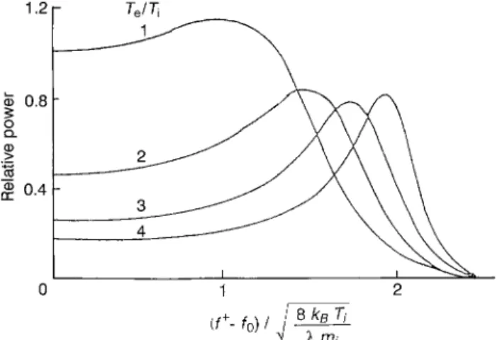
Fig. 1. Incoherent-scatter spectrum for different values of ¹e/¹i (taken from Evans, 1969)

lies between 1 and 3 demonstrates that:

B"4.8

j

S

8kB¹i_mi , (2)

where ¹i is the ion temperature in the plasma, and mi is the ion mass (Fig. 1). Figure 1 also demonstrates that if a simple trapezoid is fitted to the theoretical spectra, then the band-width occupied by each sloping side of the spectrum would range from +B/3.5 for ¹e/¹i"1 to +B/7.5 for ¹e/¹i"3. Uncertainty in this factor is the major limitation in this simple method, but the value of B/4 assumed by du Castel and Vasseur (1972) is a reasonable estimate.

For measurements in the F region, dominated by O` ions with mi"16]1.6710~27 kg:

d»p"1.56Jj

A

1#2

R

BS

(¹i)0.5qrt . (3)

However, this simple formula must be corrected for the extra errors introduced when the spectrum of the back-ground ‘‘noise’’ power is subtracted from the spectrum of the combined signal plus background. If m independent background gates (with average power SNT per unit bandwidth) are averaged and subtracted from the spec-trum of the signal plus background (with average power SPT#SNT per unit bandwidth), then the variance in the signal spectrum equals the sum of the variance in the signal plus background (JMSPT#SNTN2) plus the vari-ance in the average background (JMSNT2/mN).

It follows that the rms error in the signal spectrum is increased by a factor of:

SA

1#1 m

G

SNT SPT#SNT

H

2

B

. (4)

This method also ignores the detailed shape of the spec-trum and as such corresponds to the ‘matched-filter’ method of velocity measurement, so that

d»p+1.56 · Jj

A

1#2

R

BS

(¹i)0.5qrt

SA

1#

1

mM1#RN2

B

.

(5)

The most straightforward way of comparing the theoret-ical prediction of random error in the measurement of a parameter with the error actually observed is to measure the variance in a series of independent measurements of the parameter. For ion velocity this has previously been done in two ways; now described in Sects 1.1 and 1.2.

1.1 Similar measurements at consecutive times

Williams et al. (1984) compared the plasma velocity meas-ured by EISCAT at a given time, »p, with the mean value of the two preceding and the two following measurements, S»pT. These measurements were made during quiet geomagnetic conditions, when it could be safely assumed that the true value of the ion velocity was changing slowly and steadily, so that the mean-square value of (»p!S»pT) was equal tod»2p, the variance is the measured velocity, multiplied by 1.25.

The variance in the measured velocity was, in turn, equal to the sum of the variance due to noise, assumed proportional to (1#2/R)2, and the ‘‘geophysical’’ vari-ance due to any non-linear change of »p with time. The measurements were therefore binned according to the different values of R in the data set, and when the average variance for each bin was plotted against the correspond-ing value of (1#2/R)2 there was a high correlation. The relationship covered a wide range of signal-to-noise ratio, including relatively high values for the monostatic mea-surements made at Tromsø and relatively low values for the bistatic measurements made at Kiruna and Sodankyla¨. Using pulses of length 360ls, at a wavelength of 0.32 m, and a ‘matched-filter’ analysis programme, Will-iams et al. (1984) derived the following empirical formula, amended from the form originally published to replace

Rf, the signal-to-noise ratio over the bandwidth of the

receiver, by R, the signal-to-noise ratio over the band-width of the signal1:

d»p"278

A

1#2

R

B

1

J(rt). (6)

1 Because noise power that lies outside the signal bandwidth but inside the filter bandwidth does not contribute to the measurement error, R should be determined over the bandwidth of the scattered signal, B, not over the equivalent receiver bandwidth, Bf (which in EISCAT is twice the filter bandwidth used in the two channels of the base-band amplifier). This is obvious if a digital filter of width B is applied to the sampled data. Several previous papers on this topic, including Williams et al. (1984), have not emphasised this crucial distinction, but this is the ‘‘frequency-domain’’ equivalent of the minimum lag resolution indicated by Vallinkoski (1988, 1989). The ‘‘signal-to-noise’’ actually quoted in the standard EISCAT analysis programmes is the signal-to-noise ratio over the equivalent receiver bandwidth, Bf, which in the EISCAT common programme CP4 and in the UK special programme POLAR is equivalent to 2]50 kHz"100 kHz. Before applying Eq. 4, the measured signal-to-noise must therefore be corrected by the following relationship:

R"Rf ·BfB

"

Rf · Bf ·4.8j ·

S

_8kB¹imi "_{0.00104 ·}Rf · Bf

J¹i .

(4)

In this 1984 paper the variation with ¹e and ¹i was not considered, nor the additional noise introduced by sub-stracting background gates, so no exact comparison is possible between the theoretical formula Eq. 5 and the empirical formula Eq. 6, though there would be good agreement for ¹i+1000 K. The most important result from this paper was the good linear relationship between

d»p and (1#2/R).

1.2 Simultaneous measurements at different heights along the same magnetic field line

Jones et al. (1986) used an alternative method to esti-mate the random error in any measurement of plasma velocity: they compared simultaneous measurements of the component of ion velocity perpendicular to the mag-netic field line at different heights along the same magmag-netic field line.

The measurements were taken from the EISCAT Com-mon Programme CP2, where the beam of the Tromsø antenna was scanned in turn to four positions. After interpolation in time between consecutive measurements in a given direction, three simultaneous values of the components of ion velocity at a given height were com-bined to give an estimate of the component of plasma velocity perpendicular to the field line at that height. This procedure was repeated for eight independent heights between 210 and 580 km.

Assuming that in the F region each magnetic field line is at a single potential, then after making a small correc-tion for the change in magnetic-field strength with height (»pJ1/JB), it can be assumed that each component of field-perpendicular velocity is actually constant with height. It follows that the scatter of individual values of the corrected field-perpendicular velocities at different heights about the mean value is a measure of the random errors due to noise.

This so-called monostatic method of measuring the full vector of the ion velocity is, of course, subject to systematic errors due to spatial and temporal vari-ations, but in the absence of strong auroral activity these will affect simultaneous measurements at different heights in the same way, so that the method is valid for determining the level of noise errors in the measure-ments.

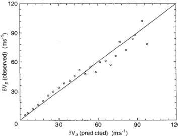
Forty thousand separate measurements of this kind were used in a full statistical analysis. The results were binned according to the value of R, and when the average rms deviation for a given value of R was plotted against the corresponding value of (1#2/ R), Jones et al. (1986) were able to confirm a linear relationship with great accuracy (Fig. 2).

As in the case considered by Williams et al. (1984), pulses of legth 360ls were used at a wavelength of 0.32 m, with a ‘‘matched-filter’’ analysis, and the following empiri-cal formula was derived:

d»p"270

A

1#2

R

B

1

J(rt). (7)

Fig. 2. Relationship between the signal-to-noise ratio over the signal bandwidth, R, of observations at different heights along the Tromsø magnetic field line and the rms random error in the corresponding components of plasma velocity perpendicular to the field line west-ward (o) and southwest-ward (K) (M is a numerical factor involved in the matrix conversion from the actual measurements to the perpendicu-lar components of velocity); based on Jones et al. (1986)

This result was also very close to the value predicted by Eq. 5 forj"0.32 m, ¹i"1000 K, m"5 and R ranging from 0 to 1. However, this early work suffered limitations in both the theoretical formula and in the empirical measurements of random noise errors.

The theoretical formula was based on the simple trap-ezoid spectrum proposed by du Castel and Vasseur (1972), and depended on the proportion of the total bandwidth which was occupied by the sloping sides of the spectrum. In reality this factor depends on the ratio ¹e/¹i, and a full theory should be based on the actual ion-acoustic spectra observed by incoherent-scatter radar, and this implies a ‘‘full-fit’’ analysis of the measured spectrum.

Moreover, the two methods of measuring the random noise error suffered the limitation that the independent measurements of velocity were made at different times or for different volumes of plasma. These limitations would be avoided if independent measurements of the same volume of plasma were made simultaneously — for example, by duplicating the measurements at different, closely spaced frequencies. Such measurements were made in the early runs of the UK special programme POLAR, and also in the early runs of the common programme CP4.

The present paper therefore develops a complete the-ory of the noise errors, and compares the predictions of this theory with the scatter actually observed between simultaneous measurements of ion velocity made at six different frequencies during a run of CP4.

2 Full theory of noise errors in the measurement of plasma velocity

The full theory of noise errors in the measurement of plasma velocity must be based on the actual spectra

(5)

observed by incoherent-scatter radar. Figure 1 shows the range of spectra predicted for values of ¹e/¹i ranging from 1.0 to 4.0. It is obvious on inspection that whereas the trapezoid approximation is reasonable for ¹e/¹i"1.0, it is increasingly inappropriate as this ratio increases. The accuracy of velocity measurement depends on the ‘‘sharp-ness’’ of the gradient of spectral power versus frequency, so as ¹e/¹i increases we would expect the actual random errors to fall below the value predicted by du Castel and Vasseur (1972). To derive a simple semi-empirical formula for this, the following procedure was followed, applying the basic method proposed by du Castel and Vasseur to the actual ion-acoustic spectra.

Let P( f )"signal power/unit bandwidth at frequency

f, SPT"average signal power over total bandwidth B (where B"(4.8/j) J8kB¹i/mi), PT"total signal power

df , (9)

and the measured component of velocity, »p, is given by the expression: »p"j2D"! j 2 [P( f`)!P( f ~)]df 2 [(LP/Lf )f_`]df . (10) In any power measurement P@ for a bandwidth d f, averaged over a time qrt (where r pulses of length q are transmitted per second for an integration time of

t seconds), the rms uncertainty in the measurement is

given by: dP@ P@" 1 J(qrtdf ), (11) (dP@)2" P@2 (qrtdf ), (d[(P( f `)#SNT)df ])2"(P( f`)#SNT)2df 2 (qrtdf ) . (12)2 Variance in the measurement of P( f`)df is then given by:

p`2"(P( f`)#SNT)2df 2

(qrtdf ) . (13)

Variance in »p derived from these two bandwidths: p2"j2 16 2 (qrtdf ) (P( f`)#SNT)2df 2 [(LP/Lf )2f_`]df 2 . (14) Therefore: 1 p2" 8(qrt) j2 (LP/Lf )2f_`df (P( f`)#SNT)2. (15) In combining the results from all pairs of bandwidths across the whole spectrum, the estimate of »p from each pair must be weighted by the appropriate value of 1/p2, andR2, the variance in the final value of »p, is equal to 1/R(1/p2). S»pT" 2(qrt) j B@2 : 0 [P( f`)!P( f ~)] (LP/Lf )f_` (P( f`)#SNT)2 Lf 8(qrt) j2 B@2 : 0 (LP/Lf )2f_` (P( f`)#SNT)2Lf " j 4 B@2 : 0 [P( f`)!P( f ~)] (LP/Lf )f_` (P( f`)#SNT)2 Lf B@2 : 0 (LP/Lf )2f_` (P( f`)#SNT)2Lf , (16) and R2" j2 (8qrt) 1 B@2_: 0 (LP/Lf )2f_` (P( f`)#SNT)2Lf . (17)

The right-hand-side expression in Eq. 17 consists of two functions. The first, a function ofj, q, r and t, depends on the wavelength used by the radar and the experiment design. The second, a function of P( f ) andSNT, depends on the signal-to-background ratio of the measurements and on the shape of the spectrum — itself a function of electron and ion temperature.

2 In practice, of course, we actually measure [P( f `)#SNT]df and subtract an estimate ofSNT based on the average noise power in

m independent background gates:

C

P( f`)#SNT! +

i/150mNi/m

D

df .

In the ideal case we can assume m to be very large, so that the additional variance added by the subtraction of background noise power is very small. In reality m is often as small as 5 and the correction indicated in Eq. 4 must be applied. For simplicity this factors is omitted in the following development of the theory but added to the final formula.

(6)

The theoretical variation of P( f ) with frequency is known for all reasonable values of ¹e and ¹i (Fig. 1), so for a given value of R (the signal-to-noise ratio over the bandwidth B"(4.8/j)J8kB¹i/mi) Eq. 17 can be integ-rated to give the rms noise error in the velocity measure-ment. In order to express this integration in a simple and memorable form, the results were equated with a modified version of the formula derived by du Castel and Vasseur (1972):

d»p"Jj

C

1#2

R

D

(¹i)0.25(qrt)0.5 F

A

¹e_¹i

B

. (18) When this calculation was carried out for all values of ¹e/¹i ranging from 1.0 to 3.0, the following simple formula gave results which agreed with the full integration to better than 2% in every case:

F

A

¹e

¹i

B

"1.17

A

1!0.16 ·¹e

¹i

B

. (19)

If we now introduce the term representing the extra noise errors introduced by the subtraction of the background noise power the equation is as follows:

d»p"1.17 Jj

C

1#2 R

D

(¹i)0.25(qrt)0.5 ]

A

1!0.16¹e ¹i

B SA

1# 1 mM1#RN2

B

. (20)

There is one final correction that must be applied, following the procedure just outlined with one extra step. In a real incoherent-scatter experiment, the spectrum ac-tually measured is the spectrum of the ion-acoustic waves in the scattering volume convolved first with the spectrum of the transmitted pulse and then with the spectrum ap-propriate to the ‘‘gating’’ of the ACF in the correlator (Rishbeth and Williams, 1985). In other words, the inte-gral indicated in Eq. 17 should be applied to the final spectra recorded by the receiver rather than the theoret-ical ion-acoustic spectra shown in Fig. 1.

The effect of each convolution is to broaden the signal bandwidth and smooth the sharp peaks in the spectrum. As these sharp peaks make the biggest contri-bution to the velocity measurement, the overall effect of convolution is to increase the rms error in the measure-ment of ion velocity. After calculating the effect of these two convolutions, the spectrum of the final output can be determined for any values of ¹e and ¹i, and by repeating the integration given in Eq. 17 the rms noise error in a velocity derived from the convolved spectrum can be calculated3.

In the case of the experiments POLAR and CP4, the original pulse length q equals 500 ls, and for the data analysed for the present paper the sampled echoes were sorted into gates each 500ls long. The effect of the double

3 Frequency convolution is the one process which is more straight-forward to study in the time domain where it corresponds to a simple multiplication of the ACF.

convolution for ¹i"1000 K was to increase the predicted rms error by 14%. d»p"1.32 Jj

C

1#2 R

D

(¹i)0.25(qrt)0.5 ]

A

1!0.16¹e ¹i

BSA

1# 1 mM1#RN2

B

. (21)

Obviously the effect of convolution increases as the pulse length decreases. After repeating the procedure for differ-ent values ofq in the range 250—1000 ls, and assuming in each case that each ‘‘gate’’ in the final output is equal to the original pulse length, it is possible to quote an empiri-cal formula for this effect which is correct to within a few percent:

d»p"1.17 Jj

C

1#2

R

D

(¹i)0.25(qrt)0.5

A

1!0.16¹e_¹i

B

p p snr sharpness of peaks ]

A

1#7.10~3 j qJ¹i

BSA

1# 1 mM1#RN2

B

. (22) p p

convolution additional error effect for pulse due to background lengthq gates

3 Estimates of errors in velocity measurement using data from the CP4 experiment

The ideal way to determine the variance in measuring ion velocity is to make the measurements simultaneously from the same volume of plasma. This was done, for example, in the POLAR experiment (van Eyken et al., 1984), where in each duty cycle pulses of length 500ls were transmitted at n different frequencies (where n was usually 4, 5 or 6). The same basic experiment was later adopted as an EISCAT Common Programme, CP4, and this programme has run regularly since 1988.

In the early versions of POLAR and CP4, a very simple correlator programme was used to determine the ACFs, first gating the sampled echoes and then determining the correlation coefficients separately for the data in each gate. This procedure introduces a second convolution in the recorded spectrum and, as already indicated, increases the random error in the measurement by a few percent. However, using such a simple programme the EISCAT correlator was able to process the different channels sep-arately so that the data taken simultaneously at different frequencies could be independently analysed.

Roberts (1970) first pointed out that a better procedure would be to determine all the cross-products of a correla-tion funccorrela-tion before ‘‘gating’’ the received signals, and this philosophy was the basis of the UNIPROG and GEN programmes devised by Turunen (1985). Eventually CP4 adopted one of these programmes. Unfortunately, with

(7)

these programmes the limitations of the EISCAT correla-tor made it impossible to process the different channels separately, and so similar data at different frequencies were added together in the correlator. As a result, only data taken during early runs of CP4 are suitable for the analysis of the random variations in the velocity measure-ments between the different channels. However, these data have proved entirely adequate to test the theoretical pre-diction summarised in Eq. 21.

When the echoes received at the different frequencies are analysed separately they give independent estimates »p as well as independent estimates of electron and ion temperature, all made with approximately the same R. For such measurements made simultaneously at n differ-ent frequencies, the mean velocity is given by:

S»pT"+ni/1»p,i

n , (23)

and this can be used to make an estimate of the rms error observed in the individual measurements during a given integration period:

d»2p"(+ni/1[»p,i!S»pT]2)

(n!1) . (24)

The aim of the exercise is therefore to compare the meas-ured value ofd»2p with the corresponding value predicted by Eq. 22, using mean values of ¹e, ¹i and R averaged over the n channels.

In making this comparison, it must be remembered that whereas each single set of measurements provides an unbiased estimate ofd»2p so that the mean value of a large set of estimates will give the true value of this parameter, the individual estimates ofd»2p will follow a s2 distribu-tion on n!1 degrees of freedom.

The predicted values ofd»2p for each set of measure-ments are therefore used to define a series of narrow ‘‘bins’’ covering the whole range of values obtained from Eq. 22. Each measured estimate ofd»2p is then put into the appropriate bin, and when all the data have been analysed a mean value ofd»2p can be determined for each bin.

In practice, to provide a rugged comparison protected from a small number of maverick points, it is better to determine the median value ofd»2p in each bin and apply a correction to give an unbiased estimate of the mean value, assuming as2 distribution (for n"5 the correction factor is 1.19 and for n"6 it equals 1.14).

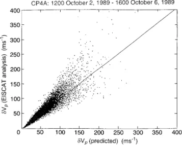
Data from 11775 separate observations during a run of CP4-A were used in the analysis. For this experiment j"0.32 m, q"500 ls, r"40 s~1, t"130 s and n"6. Figure 3 summarises the result of this analysis by plotting the measured rms value of d»p, determined in the way described, versus the predicted rms value ofd»p, distrib-uted into 25 ‘‘bins’’ covering the whole range from 0 to 100 m s~1. The agreeement between the predicted and observed values is almost perfect, giving an overall slope of 0.991 and a correlation coefficient of 99.3%.

A similar comparison was made for a limited quantity of analysed data from POLAR. The parameters of the experiment were very similar, although in this case

r"46 s~1 and f"5. Once again there was a very high

Fig. 3. Relationship between the predicted and observed values of the rms error in measuring plasma velocity (data analysed by the ‘‘full-fit’’ method)

Table 1

¹e/¹i 1 1.5 2 2.5

d»p (matched-filter)

d»p (full-fit) 1.23 1.35 1.52 1.72

correlation (99.9%) but the slope equalled 1.53. The dis-crepancy was resolved when it was discovered that these POLAR data had been analysed using a ‘‘matched-filter’’ analysis programme rather than a ‘‘full-fit’’ programme. A matched filter effectively applies poor frequency resolu-tion to the spectral analysis and consequently fails to use the full information contained in the sharpest features of the recorded spectrum. It follows that the random errors for a matched-filter analysis are considerably larger than for a full-fit analysis, especially for large values of ¹e/¹i. Table 1 indicates the increased error in velocity measure-ments for different values of ¹e/¹i.

4 Comparison with error estimates from the EISCAT analysis programme

The analysis programme used in EISCAT fits theoretical spectra to the observed ACF and derives an estimate of the random error from the variance of the deviation be-tween the observed lags in the ACF and the lags predicted. In some earlier analysis programmes these errors were underestimated because the signal spectrum was oversam-pled and the values of the ACF at adjacent lags were not independent (Breen et al., 1996; Huuskonen and Lehtinen, 1996).

To test the EISCAT analysis programme used for CP4, the rms error quoted in the output from the analysis programme was compared with the rms error predicted by Eq. 22, using the measured values of ¹e and ¹i. The results are plotted in Fig. 4, which demonstrates two factors. First, the mean values of the errors quoted by the analysis programme agree very well with the error

(8)

Fig. 4. Relationship between the individual errors quoted by the EISCAT analysis programme and the values derived by the theoret-ical formula

predicted by Eq. 22, which is a strong vindication of the theory applied both in the analysis programme and in the error estimate. The second point that emerges from the comparison is that the error estimates derived by the analysis programme show a large scatter, and individual values may be seriously over- or underestimated. In this context the theoretical estimate of noise error given in Eq. 22 is not only useful in predicting the accuracy of any planned long-pulse experiment, but it is also a reliable estimate of the random noise error incurred in a single measurement of ion velocity.

5 Conclusion

There is remarkably good agreement between the level of random noise errors in measurements of ion velocity predicted for the actual theoretical spectrum of the re-ceived echoes, the level derived by the present EISCAT analysis programme from the variance of the signal ACF at different lags, and the level derived from the observed scatter between velocities measured simultaneously but independently at different frequencies. This agreement leads to two very satisfactory conclusions:

i) The theory outlined is essentially correct and complete, and includes all the different factors (such as back-ground subtraction, convolution on transmission etc.) that affect the final error level.

ii) It follows that to a first approximation, the observed scatter of measurements of ion velocity at closely spaced frequencies can be attributed to fundamental system noise. It is reassuring that there appears to be no other major factor contributing to this scatter, and that the measurements of ion velocity are as accurate as possible given the physical constraints of the peak transmitted power, the antenna gain and the system noise temperature.

A careful scrutiny of Fig. 3 does suggest that the slope of the observed values ofd»p versus the predicted values is

slightly greater than 1 (&1.06) for d»p(40 ms~1, but falls for greater values. The same pattern is seen in the comparison between the observed values of d»p and the mean of the values derived by the EISCAT analysis pro-gramme. As the smallest values ofd»p correspond to the highest values of R it would be anticipated that any extra source of error would have little effect on the smaller observed values ofd»p but might increase the larger ob-served values, but this is opposite to the effect obob-served. At present this effect is unexplained. It is, however, a small effect, and while this qualifies the remarkably good agree-ment reported for the data set as a whole, it remains true that the semi-empirical formula quoted in Eq. 22 is good to a few percent and as such will prove useful in helping to plan incoherent-scatter experiments, indicating the way that different factors influence the final accuracy of the velocity measurements. The analysis also indicates the extend to which a ‘‘matched-filter’’ analysis of incoherent-scatter data leads to considerably larger random errors than a ‘‘full-fit’’ analysis, especially for high values of the ratio ¹e/¹i.

Acknowledgements. The authors would like to thank the Director

and staff of EISCAT for the CP4 data used in this paper. EISCAT is a scientific association supported by the research councils of Fin-land, France, Germany, Japan, Norway, Sweden and the UK. The authors would also like to thank the referees for their careful scru-tiny of the paper and their valuable suggestions.

Topical Editor D. Alcayde´ thanks C. Lathuittere and A. Huus-konen for their help in evaluating this paper.

References

Breen, A. R., P. J. S. Williams, A. Etemadi, and V. N. Davda, Uncertainties in measurements of electron temperature and the estimation of F-region electron heat conduction from EISCAT data, J. Atmos. ¹err. Phys., 58, 145—159, 1996.

du Castel, F., and G. Vasseur, Evaluation des performances d’un sondeur ionospherique a` diffusion incoherente, Ann.

¹elecom-mun., 27, 239—247, 1972.

Evans, J. V., Theory and practice of ionosphere study by Thomson scatter radar, Proc. IEEE., 57, 496—530, 1969.

Huuskonen, A., and M. S. Lehtinen, The accuracy of incoherent scatter measurements: error estimates valid for high signal levels,

J. Atmos. ¹err. Phys., 58, 453—463, 1996.

Jones, G. O. L., K. J. Winser, and P. J. S. Williams, Measurements of plasma velocity at different heights along a magnetic field line, J.

Atmos. ¹err. Phys., 48, 887—892, 1986.

Lehtinen, M. S., Statistical Theory of Incoherent Scatter Radar Measurements, EISCA¹ ¹echnical Note 86/45, 1—97, 1986. Rishbeth, H., and P. J. S. Williams, The EISCAT ionospheric radar:

the system and its early results, Q.J.R. Astron. Soc., 26, 478—512, 1985.

Roberts, J. B. G., Spectrum analysis of ionospheric radar returns, Electron. Lett., 6, 196—197, 1970.

Turunen, T., GEN-SYSTEM — a new experimental philosophy for EISCAT radars, J. Atmos. ¹err. Phys., 48, 777—785, 1986. Vallinkoski, M., Statistics of incoherent scatter multiparameter fits,

J. Atmos. ¹err. Phys., 50, 839—851, 1988.

Vallinkoski, M., Error analysis of incoherent scatter radar measure-ments, EISCA¹ ¹echnical Note 89/49, 1—110, 1989.

van Eyken, A. P., H. Rishbeth, D. M. Willis, and S. W. H. Cowley, Initial EISCAT observations of plasma convection at invariant latitudes 70°—77°, J. Atmos. ¹err. Phys., 46, 635, 1984. Williams, P. J. S., G. O. L. Jones, and A. R. Jain, Methods of

measuring plasma velocity with EISCAT, J. Atmos. ¹err. Phys., 46, 521—530, 1984.