HAL Id: cea-02965063
https://hal-cea.archives-ouvertes.fr/cea-02965063
Submitted on 13 Oct 2020
HAL is a multi-disciplinary open access
archive for the deposit and dissemination of
sci-entific research documents, whether they are
pub-lished or not. The documents may come from
teaching and research institutions in France or
abroad, or from public or private research centers.
L’archive ouverte pluridisciplinaire HAL, est
destinée au dépôt et à la diffusion de documents
scientifiques de niveau recherche, publiés ou non,
émanant des établissements d’enseignement et de
recherche français ou étrangers, des laboratoires
publics ou privés.
Photometric redshifts for the Pan-STARRS1 survey
P. Tarrío, S. Zarattini
To cite this version:
P. Tarrío, S. Zarattini. Photometric redshifts for the Pan-STARRS1 survey. Astronomy and
Astro-physics - A&A, EDP Sciences, 2020, 642, pp.A102. �10.1051/0004-6361/202038415�. �cea-02965063�
https://doi.org/10.1051/0004-6361/202038415 c P. Tarrío et al. 2020
Astronomy
&
Astrophysics
Photometric redshifts for the Pan-STARRS1 survey
?
P. Tarrío
1,2and S. Zarattini
11 AIM, CEA, CNRS, Université Paris-Saclay, Université Paris Diderot, Sorbonne Paris Cité, 91191 Gif-sur-Yvette, France 2 Observatorio Astronómico Nacional (OAN-IGN), C/ Alfonso XII 3, 28014 Madrid, Spain
e-mail: p.tarrio@oan.es
Received 13 May 2020/ Accepted 28 July 2020
ABSTRACT
We present a robust approach to estimating the redshift of galaxies using Pan-STARRS1 photometric data. Our approach is an appli-cation of the algorithm proposed for the SDSS Data Release 12. It uses a training set of 2 313 724 galaxies for which the spectroscopic redshift is obtained from SDSS, and magnitudes and colours are obtained from the Pan-STARRS1 Data Release 2 survey. The photo-metric redshift of a galaxy is then estimated by means of a local linear regression in a 5D magnitude and colour space. Our approach achieves an average bias of∆znorm = −1.92 × 10⁻⁴, a standard deviation of σ(∆znorm)= 0.0299, and an outlier rate of Po = 4.30%
when cross-validating the training set. Even though the relation between each of the Pan-STARRS1 colours and the spectroscopic redshifts is noisier than for SDSS colours, the results obtained by our approach are very close to those yielded by SDSS data. The proposed approach has the additional advantage of allowing the estimation of photometric redshifts on a larger portion of the sky (∼3/4 vs ∼1/3). The training set and the code implementing this approach are publicly available at the project website.
Key words. galaxies: distances and redshifts – galaxies: general – methods: data analysis – techniques: photometric
1. Introduction
In the last two decades, there has been a rise in the develop-ment of large photometric surveys, like the Sloan Digital Sky Survey (SDSS,York et al. 2000), the Panoramic Survey Tele-scope & Rapid Response System (Pan-STARRS,Chambers et al. 2016), and the Dark Energy Survey (DES,Dark Energy Survey Collaboration 2016). Robust methods to estimate the redshift of galaxies from photometric data are essential to maximising the scientific exploitation of these surveys.
Two main approaches are generally used for the computation of photometric redshifts: methods based on physical models and data-driven methods. In the model-based approach, the estima-tion of the redshift is obtained by modelling the physical pro-cesses that drive the light emission of the object. The simplest and most commonly used method belonging to this category is spectral energy distribution (SED) fitting. It is based on the def-inition of an SED model, either from theory or from observa-tions, and the fitting of this model to a series of observations in different bands. The definition of an appropriate model is cru-cial to the performance of the method, therefore it requires us to take many different aspects into account (stellar population models, nebular emissions, and dust attenuation, among others). Once the model is defined, observations over the entire wave-length range are required to obtain an accurate fitting. Examples of these methods are the HYPERZ code (Bolzonella et al. 2000), the BPZ code (Benítez 2000), the LePhare code (Ilbert et al. 2006), and the EAZY code (Brammer et al. 2008).Saglia et al. (2012) also apply an SED technique to compute the photometric redshifts of galaxies using Pan-STARRS broadband photometry.
? The code and the training set are available at the project website:
https://www.galaxyclusterdb.eu/m2c/relatedprojects/ photozPS1.
In large-area photometric surveys like SDSS, Pan-STARRS, and DES, the number of photometric bands available is relatively small (5 for each of the cited surveys) and they only cover the optical part of the spectrum. Thus, if no ancillary data are avail-able, the SED fitting technique is not very robust in the deter-mination of photometric redshifts. The same issue affects the data-driven methods used in the cited surveys, but its effect can be mitigated when a large and complete training set is available (Salvato et al. 2019). On the other hand, these surveys offer a large number of extragalactic sources, and are well suited to the use of data-driven methods. These methods usually employ a supervised machine learning algorithm to estimate the unknown redshift of a galaxy from broadband photometry. Supervised algorithms require a (large) set of reliable spectroscopic red-shifts that are used to learn how redred-shifts correlate with colours. Some examples of these techniques are ANNz (Collister & Lahav 2004), ANNz2 (Sadeh et al. 2016), TPZ (Carrasco Kind & Brunner 2013), GPz (Almosallam et al. 2016), METAPhoR (Cavuoti et al. 2017), or the nearest-neighbor color-matching photometric redshift estimator ofGraham et al.(2018).
Another example of a machine learning approach to the com-putation of photometric redshifts is presented in Beck et al. (2016); a large sample of galaxies (about 2 million) with both photometric and spectroscopic information is used as a train-ing set to estimate the redshift of all the galaxies in SDSS Data Release 12 (DR12,Alam et al. 2015) using a local linear regression. A similar method was also presented inCsabai et al. (2007) and in earlier SDSS releases. Nowadays, these photomet-ric redshifts from SDSS are widely used in a variety of scientific publications. Examples include the validation of galaxy clus-ters (Streblyanska et al. 2018), the clustering of galaxies (Ross et al. 2010), the study of faint dwarfs in nearby groups (Speller & Taylor 2014), the study of luminosity functions in galaxy
Open Access article,published by EDP Sciences, under the terms of the Creative Commons Attribution License (https://creativecommons.org/licenses/by/4.0),
clusters (Goto et al. 2002), binary quasar selection at high red-shift (Hennawi et al. 2010), supernovae type Ia studies (Rodney & Tonry 2010), neutrino counterpart detection (Reusch et al. 2020), or gamma ray burst validation (Ahumada et al. 2020). The robust-ness of the SDSS redshift estimation algorithm is well established. The goal of this paper is to apply theBeck et al.(2016) algo-rithm to compute photometric redshifts using the Pan-STARRS1 (PS1) photometric data, which cover an area that is twice as large as the SDSS footprint and with magnitude limits about two mag-nitudes fainter than the SDSS ones. The SDSS and PS1 surveys have four photometric bands in common, plus a different fifth band that is on the bluer side of the spectrum for SDSS and on the redder side for PS1. To apply theBeck et al.(2016) algorithm to PS1, we thus needed to select the appropriate PS1 photometric data that allow us to compute the redshift, to construct a proper training set, and to reassess the performance of the linear regres-sion algorithm when using this information. The training set and the code implementing the PS1 photometric redshift approach presented in this paper has been made available for the commu-nity at the project website.
The approach proposed in this paper was initially designed with the purpose of confirming cluster candidates of the Com-bined Planck-RASS (ComPRASS) catalogue (Tarrío et al. 2019). This all-sky catalogue of galaxy clusters and cluster can-didates was validated by careful cross-identification with pre-viously known clusters, especially in the SDSS and the South Pole Telescope (SPT) footprints. Still, many candidates remain unconfirmed outside these areas. Having information on the pho-tometric redshifts in the PS1 area will enable us to confirm Com-PRASS candidates in this region. Furthermore, the greater depth of PS1 compared to SDSS allows us to better detect the over-densities associated with the clusters, and therefore to obtain a more robust estimation of their richness. The photometric red-shifts of PS1 will also facilitate the extension of other scientific studies performed with SDSS photometric data to the area of the sky covered by PS1. Some examples are studies related to the formation and evolution of galaxies, or to the properties of dark energy (Salvato et al. 2019).
The paper is organised as follows: Sect.2 summarises the linear regression method and how it is applied to PS1 data. Section3describes the procedures that we put in place to prepare the training set using PS1 photometry and SDSS spectroscopy. Section 4 evaluates the performance of the proposed redshift estimation approach. Section 5presents a comparison with the results obtained using different photometric data from PS1 and SDSS. Section 6 gives some practical notes on the use of the method and the associated dataset. Finally, Sect.7concludes the paper with a summary of the main results.
2. Redshift estimation approach
In this Section, we describe our approach to estimate the redshift of galaxies from PS1 photometric data. The proposed approach is an application of the linear regression method used in the SDSS DR12 (Beck et al. 2016) to the PS1 dataset, and thus, it can be used to calculate photometric redshifts for all galaxies in the PS1 footprint (∼3/4 of the sky). Similarly toBeck et al.(2016), our approach is data-driven and uses a training set T composed of galaxies with known spectroscopic redshifts and a set of magni-tudes and colours, which are obtained in our case from the PS1 survey. The redshift of a galaxy is estimated by means of a local linear regression in a D-dimensional magnitude and colour space. The rest of this Section summarises the linear regression algorithm fromBeck et al.(2016) (Sect.2.1) and describes, in
detail, the magnitude-colour space that has been selected for our approach (Sects.2.2and2.3). We also explain how we deal with the potential problem of missing information (Sect.2.4).
This approach has been designed to work on both Data Release 1 (DR1) and Data Release 2 (DR2), although in this paper we present the results corresponding to DR2. The perfor-mance for DR1 data was also tested, finding no significant dif-ferences.
2.1. Linear regression algorithm
The local linear model ofBeck et al.(2016) establishes that the redshift of a galaxy can be written as a linear combination of D galaxy properties (magnitudes and colours), hereafter features, x1, ..., xD, as follows:
z= xTθ, (1)
where x = [1, x1, ..., xD]T is the feature vector of the galaxy.
The column vector θ contains the D+1 coefficients of the D-dimensional linear regression, with its first element rep-resenting a constant offset. The coefficient vector θ can be estimated by constructing an over-determined system of k equa-tions using k galaxies of the training set T : zspec = Xθ, with
zspec= [z(1), ..., z(k)]T being the spectroscopic redshifts of the k
chosen galaxies, and X= [x(1), ..., x(k)]Tthe corresponding k
fea-ture vectors. The least-squares solution of this system is then: ˆ
θ = (XTX)−1
XTzspec. (2)
The error of the photometric redshift can be estimated from the difference between the spectroscopic redshifts of the k galax-ies and the corresponding photometric redshifts provided by the regression: δzphot = s P k(zspec− Xˆθ)2 k . (3)
To apply this method, it is necessary to define how to chose the k training galaxies used to estimate θ, and to define the D features that characterise each galaxy.
In our case, the k galaxies are chosen to be the nearest neigh-bours of the target galaxy in terms of Euclidean distance in the D-dimensional space. In particular, we chose k= 100, as inBeck et al.(2016). Additionally, in the case that some of these k neigh-bours have outlying redshifts (|z( j)spec−x( j)Tθ| > 3δˆ zphot), we discard
them and repeat the computation of ˆθ (Eq. (2)) using the remain-ing l < k neighbours. We note that, in some cases, a galaxy can fall outside the D-dimensional bounding box of its nearest neigh-bours. In these cases, Eq. (1) constitutes an extrapolation, so the results may be less reliable. The impact of the extrapolation on the estimated photometric redshift is evaluated in Sect.4.2. Our code provides a flag to indicate these cases.
2.2. Choice of input features
The key point to successfully employ the linear regression algo-rithm described in Sect.2.1(see alsoBeck et al. 2016) with PS1 photometric data is to appropriately select the D features to be used. The SDSS and PS1 surveys have both imaged the sky using five broadband filters. Four of these filters (g, r, i, and z) are similar in both surveys, although with some minor differences (Tonry et al. 2012). The fifth filter, however, is completely dif-ferent: SDSS uses the u filter, which covers the bluest part of
the measured spectrum (at bluer waveleghts than the g filter), whereas PS1 uses the y filter, which spans the reddest part of the spectrum (at redder wavelengths than the z filter). The method defined inBeck et al. (2016) uses the SDSS r magnitude, and the u − g, g − r, r − i, and i − z colours to define the 5D space in which the linear regression takes place to estimate the red-shift. Since the u-band is not available in PS1, a natural choice inspired byBeck et al.(2016) is to use the PS1 r magnitude, and the four colours that can be constructed with consecutive mag-nitudes, which are g − r, r − i, i − z, and z − y. These are the five features that we decided to use in our method. However, it is worth noting that other combinations of the five bands are also possible without a significant difference in the results, given that all the photometric information is included.
The PS1 database provides several ways of measuring mag-nitudes and fluxes of objects in its five photometric bands. We used stack photometry, since it provides the best signal to noise, according to Magnier et al. (2019). Then, different photomet-ric measurements are available: (i) PSF magnitudes are obtained from fitting a predefined PSF form to the detection. These mag-nitudes are especially relevant for point sources (e.g. stars). (ii) Kron magnitudes are inferred from the growth curve, after deter-mining the Kron radius of the object. These magnitudes are espe-cially relevant for non-point sources. (iii) Aperture magnitudes measure the total count rate for a point source based on integra-tion over an aperture plus an extrapolaintegra-tion involving the PSF. According to the PS1 database documentation, this photometry should not be used for extended sources, so we did not use it in our method. (iv) Fixed-aperture measurements refer to the flux measured within several predefined aperture radii (1.03, 1.76, 3.00, 4.63, and 7.43 arcsec).
Kron magnitudes are the most appropriate for extended objects like galaxies, so we chose to use the r-band Kron magni-tude for defining our r feature. Regarding the four colour features (g − r, r − i, i − z, z − y), we considered two different approaches: they can be calculated either from (a) fixed-aperture fluxes, or (b) from Kron magnitudes.
The first approach (aperture colours) computes the four colours within a fixed aperture. To obtain the aperture magni-tudes within the most appropriate aperture, we selected for each galaxy the g, r, i, z, and y fixed-aperture fluxes corresponding to the closest aperture to the r-band Kron radius of the galaxy (rkro-nrad). Then, the five selected aperture fluxes were converted into aperture magnitudes.
The full PS1 dataset files available for direct download do not provide the above-mentioned fixed-aperture fluxes, which need to be queried to the database. Instead, they provide Kron magni-tudes. As an alternative approach, we evaluated the use of these magnitudes to compute the four colours required by our method. We note that the colours constructed from the Kron magnitudes are not physically motivated, since the five different magnitudes are not measured within the same aperture. However, we will show that they provide very similar results to the ones obtained when using the fixed-aperture colours defined above, so for con-venience, we added this alternative to our code. Unless other-wise stated, the results presented in this paper were obtained with the aperture colours calculated from the fixed-aperture fluxes. We include a comparison between the different approaches in Sect.5. 2.3. Feature computation
Before calculating the five features, we need to apply a dered-dening correction to the downloaded or calculated magnitudes. Reddening is produced by the scattering of the light by dust in
the interstellar medium, and it depends on the position of the object in the sky. Therefore, it has to be corrected in order to obtain magnitudes that are more correlated with redshift.
We obtained this correction in the following way: firstly, we computed the colour excess E(B − V) for each galaxy using the Schlegel et al.(1998) maps; then, we obtained the extinction Aλ
for the g, r, i, and z bands by multiplying the colour excess by the values presented in Table 22 ofStoughton et al. (2002) for the g, r, i, and z SDSS filters, respectively, which are very similar to the ones used in PS1. For the y band, which is not present in SDSS, we calculated the extinction using the parametrisation of Fitzpatrick(1999) taking the effective λ of the y band (λeff =
9620 Å) presented in Table 4 ofTonry et al.(2012).
We then applied the dereddening correction (g= gdownloaded−
Ag, and equivalently for the other bands), and we computed the
five features (g − r, r − i, i − z, z − y, and r).
Each dimension was then standardised, by removing the mean and dividing by the standard deviation of the training set T , whose construction is described in Sect. 3. In this way, all the features span similar ranges, and, thus, contribute to a simi-lar extent to the linear regression. This feature scaling is a com-mon practice in algorithms that use Euclidean distance, like ours, since otherwise the feature with a larger scale (the magnitude in our case) would dominate the computation of the distance.
We note that the zero-point correction that is usually taken into account in public software for the computation of photo-metric redshifts does not need to be included in our method. The reason is that our method is not sensitive to the addition of con-stant terms to the features, since it uses standardised features. 2.4. Missing features
The PS1 dataset contains galaxies for which one or more magni-tudes may not be available, resulting in missing features. Missing features can occur due to occasional photometric measurement errors produced by artifacts or other problems in the image, or because the galaxy is too faint to be detected in a given band (usu-ally in the more extreme bands, g or y). In any case, galaxies with missing features can still be reasonably well represented by their remaining available features. The redshift estimation approach described above can still be applied to estimate the photomet-ric redshift of these galaxies in several ways. In particular, we decided to calculate the redshift of such galaxies by using only the available features, that is to say, we construct the feature vec-tor x with D0 < D features, both for the target galaxy and the
training galaxies, and then use Eqs. (1) and (2) as before. In this way, we use the subset of the training set T that has all the five features available (T5) to calculate the redshift of a galaxy that
has the five features. Likewise, when a galaxy is missing one fea-ture, we also use T5as training set, but we do not consider the
missing feature in any of the training galaxies. Another possible approach to follow in the case of a missing feature in the target galaxy could be to use the subset of T that has the other 4 features available as training set (T4, with T5 ⊂ T4 ⊂ T ). In this paper,
we report the results corresponding to the first approach, but we note that the second option produces similar results and is also available in the code.
It is worth mentioning that, for simplicity, the standardisa-tion of the features is done in any case with the mean and the standard deviation of the subset T5. We verified that other
rea-sonable choices (e.g. using, for each feature, the mean and the standard deviation of all the galaxies containing that feature) do not yield any significant difference in the results. In Sect.4.4, we evaluate the performance of our redshift estimation approach in the case of missing features.
Table 1. Parameters downloaded from PS1 and SDSS databases.
Parameter Database Table Description
ObjID SDSS Beck et al.(2016) Object ID in SDSS
RA SDSS Photoprimary RA in SDSS
Dec SDSS Photoprimary Dec in SDSS
ObjID PS1 StackObjectThin Object ID of closest object in PS1
Distance PS1 – Distance between SDSS and PS1 positions
RA PS1 StackObjectThin RA in PS1
Dec PS1 StackObjectThin Dec in PS1
{g, r, i, z, y}KronMag PS1 StackObjectThin Kron magnitudes
{g, r, i, z, y}KronMagErr PS1 StackObjectThin Kron magnitudes errors
primaryDetection PS1 StackObjectThin Primary stack detection flag
rKronRad PS1 StackObjectAttributes Kron radius in r band
{g, r, i, z, y}c6flxR{3,4,5,6,7} PS1 StackApFlxExGalCon6 Fluxes within 5 different apertures {g, r, i, z, y}c6flxErrR{3,4,5,6,7} PS1 StackApFlxExGalCon6 Errors in aperture fluxes
3. Construction of the training set
T
The training set ofBeck et al.(2016) included more than two million galaxies with spectroscopic redshifts. In this work, our goal was to use the same training set, but with features obtained from PS1 magnitudes instead of SDSS. To construct it, we made use of the CasJobs tool in SDSS, which allowed us to query both the SDSS and the PS1 databases. In the catalogue ofBeck et al.(2016), each galaxy is identified via its ObjID (a unique number assigned to each object in the SDSS database). Thus, our first step was to obtain the coordinates for each object using an appropriate query to the SDSS database. Then, we performed a query in the PS1 database (Flewelling et al. 2019) to look for the PS1 object nearest to each SDSS object. This was done using the fGetNearestObjEq function, and limiting the search to a radius of 3000. This conservative choice allowed us to define, a
posteriori, the matching distance up to which we can consider the match reliable. Objects with greater matching distances are not kept in the training set. We show later that this maximum distance was fixed to 100.
Our query produces the following output parameters: the identifier (ObjID) and coordinates (RA, Dec) of the object in both the SDSS and PS1 databases, the distance between the two positions, the g, r, i, z, and y Kron magnitudes and their asso-ciated errors in the PS1 database (using stack photometry), the PS1 primarydetection flag, the Kron radius measured in the PS1 rband, and the g, r, i, z, and y PS1 fluxes measured within the five predefined aperture radii (1.03, 1.76, 3.00, 4.63, and 7.43 arcsec) and their associated errors. Table1lists these parameters and the tables where they are available.
The training set T is constructed from this catalogue, after cleaning it for unwanted objects, calculating the five features defined in Sect.2, and taking the spectroscopic redshift from the catalogue ofBeck et al.(2016). In the following sub-sections, we describe these steps in detail.
3.1. Cleaning
The catalogue resulting from the query to the PS1 database con-tains some duplicate entries, i.e. objects with the same ObjID and the same or different properties. We cleaned this catalogue from these objects by keeping only one object for each ObjID.
In particular, we selected the ones for which primarydetection was equal to 1, which indicates that the entry is the primary stack detection. If there was more than one object satisfying this condi-tion, we selected the one with more magnitudes available. Exact duplicates were also removed.
We additionally removed from the downloaded catalogue two classes of objects. The first class corresponds to objects for which PS1 and SDSS photometry are very different. PS1 and SDSS have four photometric bands in common (g, r, i, and z), so we expect to have a small difference between the magni-tudes in those four bands measured by PS1 and SDSS. How-ever, we noticed that our catalogue included some objects for which the difference between these magnitudes was very high (even more than ten magnitudes in some cases). As a precaution, we decided to exclude them from our training set. In particular, we excluded objects for which the difference between any SDSS magnitude and the corresponding PS1 magnitude is greater than 4.
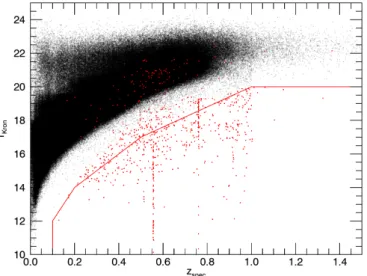
The second class of excluded objects corresponds to those that appear to be too bright for their assigned spectroscopic red-shift. We noticed the presence of very bright objects at high redshift in our catalogue that are not physically possible (e.g. r = 12.1 at z = 0.82). After a visual inspection in SDSS, we found that these objects were indeed bad samples due to two main reasons: (a) low-redshift star-forming galaxies with wrong (high) SDSS spectroscopic redshift; and (b) wrong magnitude measurements (for example, in galaxies affected by the light of close-by saturated stars, or by external regions of foreground extended galaxies). We decided to remove these objects by set-ting, for each magnitude, the limits in the magnitude-redshift relations given in Table 2. Figure 1shows the magnitude lim-its for the r-band, together with the galaxies that were removed after applying the different magnitude limits.
Figure2shows the distribution of distances between the PS1 and SDSS objects in the cleaned catalogue. The scale is loga-rithmic to highlight that there is a small tail of objects far away from the SDSS position, as allowed from our large search radius (3000). Since our goal is to keep only the objects for which the match is secure, we removed all the objects whose distances to the SDSS positions were larger than 100from our sample. These were 2368 objects out of 2 316 092 (corresponding to ∼0.10%), resulting in a training set T with 2 313 724 objects. This conser-vative approach allows us to safely use the SDSS spectroscopic redshift with the PS1 magnitudes.
Table 2. Magnitude limits for different redshift ranges.
Magnitude limit Redshift range g = 11.00 + 20.00 zspec 0.1 < zspec< 0.2 g = 12.33 + 13.33 zspec 0.2 < zspec< 0.5 g = 17.75 + 2.50 zspec 0.5 < zspec< 0.9 g = 20.00 zspec> 0.9 r= 10.00 + 20.00 zspec 0.1 < zspec< 0.2 r= 12.00 + 10.00 zspec 0.2 < zspec< 0.5 r= 14.00 + 6.00 zspec 0.5 < zspec< 1.0 r= 20.00 zspec> 1.0 i= 10.00 + 20.00 zspec 0.1 < zspec< 0.2 i= 12.00 + 10.00 zspec 0.2 < zspec< 0.4 i= 14.00 + 5.00 zspec 0.4 < zspec< 1.0 i= 19.00 zspec> 1.0 z= 10.75 + 12.50 zspec 0.1 < zspec< 0.3 z= 12.25 + 7.50 zspec 0.3 < zspec< 0.5 z= 14.00 + 4.00 zspec 0.5 < zspec< 1.0 z= 18.00 zspec> 1.0 y = 9.25 + 17.50 zspec 0.1 < zspec< 0.3 y = 12.25 + 7.50 zspec 0.3 < zspec< 0.5 y = 14.00 + 4.00 zspec 0.5 < zspec< 1.0 y = 18.00 zspec> 1.0
Notes. Objects with magnitudes below these limits are not included in the training set.
Fig. 1.Scatter plot of r Kron magnitude as a function of the spectro-scopic redshift for the galaxies in the training set (black dots). Red dots represent the galaxies that are removed for not satisfying the magnitude limits defined in Table2. The red line represents the magnitude limits for the r-band.
3.2. Final training set
The final training set T contains 2 313 724 galaxies. For each galaxy, the training set provides the spectroscopic redshift zspec
obtained from the catalogue ofBeck et al.(2016), and the five features (g − r, r − i, i − z, z − y, and r) obtained as explained in Sect.2.3. The features that could not be calculated due to a missing magnitude were set to a default value (−999).
The redshift distribution of the galaxies in T is shown in Fig.3, where T has been divided into two subsets: the galaxies that have the 5 features available (T5, in blue), and the galaxies
that have one or more features missing (in red). For comparison,
Fig. 2.Distribution of distances between the PS1 objects and the SDSS objects. In the final training sample T we only used objects with dis-tances smaller than 100
.
Fig. 3.Distribution of spectroscopic redshifts in our training set. In blue, we show the galaxies that have the five features available (T5). In red,
the remaining galaxies. The dashed black line shows the redshift distri-bution of the original SDSS training set.
Figure3also shows the spectroscopic redshift distribution of the original SDSS training set, which contained 2 379 096 galaxies. The PS1 training set that we present in this section is smaller than the original SDSS one, as expected when making a match between different catalogues. This difference can be due to errors in the astrometry or photometry of the two surveys, as well as to intrinsic limits of our match methodology. However, we stress that we tried to use a conservative approach in which the num-ber of galaxies is smaller, but the robustness of the match is favoured. This result was reached while loosing less than 3% of the original galaxies.
Even though PS1 is deeper than SDSS, the chosen training set is sufficient for our goals. Adding fainter or higher-redshift galaxies to the training set will not significantly improve the per-formance of our approach, since the main limitation comes from the available photometric bands. We have tested that the addition of high-redshift spectroscopic information from the Extended Baryon Oscillation Spectroscopic Survey (eBOSS) sample at z > 0.5 (∼200 000 galaxies) does not improve the estimation of the photometric redshift.
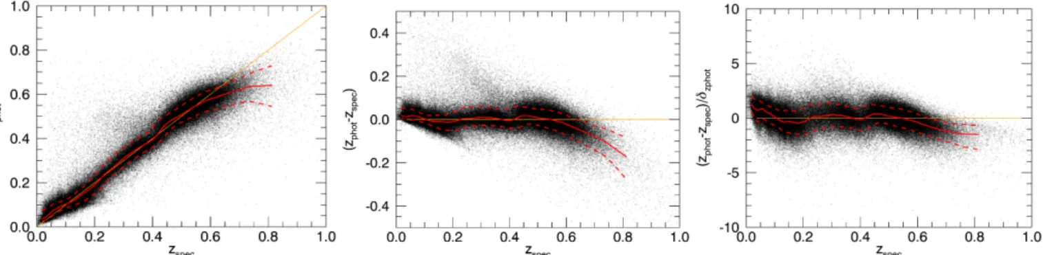
Fig. 4.Photometric redshift zphot(left), redshift error zphot− zspec(middle), and error divided by the estimation of the error provided by the method
(zphot− zspec)/δzphot(right) as a function of the spectroscopic redshift zspec. These results were obtained with a 100-fold cross-validation strategy on
the set of galaxies with the five magnitudes available (T5). The black dots represent the individual galaxies. Only 10% of the galaxies are shown,
for better visualisation. The red solid and dotted lines represent the median and the 68% confidence regions, respectively, computed for groups of 10 000 galaxies with consecutive zspec. The orange line shows zphot= zspec.
4. Performance evaluation 4.1. Overall redshift precision
To evaluate the performance of the proposed approach, we per-formed a k-fold cross-validation. We randomly divided the train-ing set T into k disjoint subsets of equal sizes. Then, we took one of the subsets as a test set, and the remaining k − 1 subsets as training set for estimating the photometric redshift of the galax-ies in the test set. The experiment is repeated k times, with each of the k subsets used exactly once as the test set. We chose to use k= 100, in such a way that the validation is performed each time on 1% of the galaxies, using the remaining 99% for training. The reasons for this choice, different from the commonly used value of k = 10, are as follows. First, with a larger value of k, the training sets used during the validation are closer to the com-plete training set T that will be used in practice for calculating redshifts of galaxies. This reduces the bias of the performance evaluation strategy. Second, given the large size of the training set, the variance of this strategy is still very low.
Figure4shows the photometric redshift zphot, the actual error
zphot− zspec, and the error divided by the estimation of the error
provided by the method (zphot − zspec)/δzphot as a function of
the spectroscopic redshift for the galaxies with the five mag-nitudes available (T5). The photometric redshift follows quite
well the spectroscopic redshift, especially in the intermediate redshift range (0.1 < zspec < 0.6), where the average bias,
∆z = |zphot− zspec|, is below 0.02 or 0.5δzphot.
For high-redshift galaxies (zspec > 0.6), the method tends
to underestimate the redshift, and also presents a higher scat-ter. This behaviour was also observed in Beck et al. (2016). The increased scatter is due to the low number of high-redshift galaxies in the training set. The negative bias is an Eddington bias produced by the limited depth of the PS1 survey: close to the detection limit, over-luminous galaxies are preferentially detected, yielding a bias towards lower redshifts. In this redshift range, 54% of the galaxies are within ±δzphotand 85% are within
±2δzphot. The percentage of galaxies in this range whose redshift
is estimated via extrapolation is 0.13%, seven times higher than the value in the intermediate redshift range (0.018%). For low-redshift galaxies (zspec< 0.1), the method tends to overestimate
the redshift, as inBeck et al.(2016). In this redshift range 65% of the galaxies are within ±δzphotand 94% are within ±2δzphot. The
percentage of galaxies in this range whose redshift is estimated
via extrapolation is 0.065%, higher than in the intermediate red-shift range, but lower than in the high redred-shift range.
In order to quantitatively compare the average performance of the proposed method to the one obtained inBeck et al.(2016), we used the same definition of the normalised redshift estima-tion error, that is∆znorm =
zphot−zspec
1+zspec . After iteratively removing
the outliers, defined as |∆znorm| > 3σ(∆znorm), the average bias
of our approach is∆znorm = −1.92 × 10⁻⁴, the standard
devia-tion is σ(∆znorm)= 0.0299, and the outlier rate is Po = 4.30%,
when calculated on the ensemble of results from the 100-fold cross-validation. The differences between the 100 individual experiments were negligible, with a standard deviation of 5% on σ(∆znorm), 4% on the outlier rate, and with average biases
always compatible with 0 (below 8 × 10⁻⁴). For reference, the results reported byBeck et al.(2016) were∆znorm= 5.84 × 10⁻⁵,
σ(∆znorm) = 0.0205, and Po = 4.11%, which are of the same
order, but slightly better than ours. We note, however, that they were calculated using a different training set, so they are not directly comparable. A direct comparison is presented in Sect.5.2.
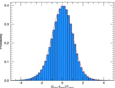
Figure 5 shows the normalised histogram of (zphot −
zspec)/δzphottogether with a standard normal distribution. The two
distributions are well in agreement, apart from a small bias (as inBeck et al. 2016, cf. their Fig. 4). This indicates that the esti-mated errors δzphot represent the accuracy of the redshift
estima-tion quite well.
4.2. Impact of the photometric errors
The errors in the measurements of the photometric magnitudes have an impact in the final accuracy of the estimated redshift. To evaluate this effect, we classified the galaxies into five different classes according to their photometric errors. Class 1 includes galaxies with low photometric errors, and Classes 2–5 include galaxies with progressively higher errors. The error limits for the different classes were manually chosen and are given in Table3. We also define an additional Class E, which includes the galaxies whose redshift is estimated via an extrapolation of Eq. (1). This occurs when the galaxy features lie outside the bounding box of its nearest neighbours, as mentioned in Sect.2.1.
The photometric error corresponding to the r-band Kron magnitude (∆r) is directly obtained from the query to the PS1 database (rKronMagErr in Table1). The photometric errors in
Fig. 5.Normalised histogram of zphot− zspec/δzphot. For reference, the red
line shows a standard Gaussian distribution.
Table 3. Photometric error limits for the defined classes.
Class ∆rmax ∆(g − r)max ∆(r − i)max ∆(i − z)max ∆(z − y)max
1 0.05 0.10 0.05 0.05 0.10
2 0.10 0.20 0.10 0.10 0.20
3 0.15 0.30 0.15 0.15 0.30
4 0.25 0.50 0.25 0.25 0.50
Notes. A galaxy belongs to a given class if its five photometric errors are below the specified values for that class and it is the lowest possible class. Class 5 contains galaxies for which one or more of the photomet-ric errors are above the limits corresponding to Class 4.
the four aperture colours are obtained from the errors in the corresponding aperture fluxes. If fg is the aperture flux in the g band and ∆ fg the corresponding error, which are obtained
from the query (rgc6flxR and rgc6flxErrR in Table1), the error in the g-band aperture magnitude is calculated as ∆g = 2.5 log(e) ×∆ fg/ fg, and analogously for the other aperture mag-nitudes. The error in the aperture colours is thus calculated as ∆(g − r) = p(∆g)2+ (∆r)2, and similarly for the other colours.
Table4summarises the performance of the redshift estima-tion for the different photometric classes. The bias is very close to 0 for all the classes, being positive for Class 1 and increas-ingly negative for Classes 2–5. This results in a slightly negative bias for the whole sample (∆znorm = −2.01 × 10⁻⁴) since, even
though the number of Class 1 galaxies dominates, the negative bias of the other classes is higher in absolute value. The standard deviation of the normalised redshift estimation error σ(∆znorm)
increases for higher photometric errors, as expected, and the same occurs with the outlier rate. For the galaxies in Class E, the bias and σ(∆znorm) is higher than for the other classes.
The defined photometric classes can be used to filter out, if needed, the galaxies for which the redshift estimation is less precise.
4.3. Impact of the position in the colour-magnitude space The position of the galaxy in the D-dimensional feature space also has an effect on the redshift estimation error. Galaxies situ-ated in dense regions are expected to have smaller errors, since
Table 4. Average normalised redshift estimation bias∆znorm, standard
deviation σ(∆znorm) and outlier rate Po for the defined photometric
classes.
Class ∆znorm σ(∆znorm) Po N
1 9.06 × 10⁻⁵ 0.0266 2.89 1 263 179 2 −7.59 × 10⁻⁴ 0.0331 3.82 464 717 3 −6.96 × 10⁻⁴ 0.0347 4.75 187 214 4 −1.68 × 10⁻³ 0.0400 7.46 127 412 5 −2.20 × 10⁻³ 0.0460 8.39 118 162 E 5.41 × 10⁻⁴ 0.1228 4.32 810 All −1.92 × 10⁻⁴ 0.0299 4.30 2 161 494
Notes. These quantities were calculated after iteratively removing the outliers, defined as |∆znorm| > 3σ(∆znorm). The number of galaxies N
(from the 100 different Ttest sets) belonging to each class is also
indi-cated.
their neighbours are very close to them in the D-dimensional colour-magnitude space, and likely have similar redshifts. On the contrary, galaxies situated in sparse regions have larger errors in the redshift estimation, since their neighbours are further away in the colour-magnitude space, and probably have a bigger dis-persion in their redshifts.
To characterise this effect, we computed several error maps that provide the redshift estimation errors as a function of the position in the D-dimensional colour-magnitude space. These error maps can be used to filter out, if required, the regions in the colour-magnitude space that have larger errors.
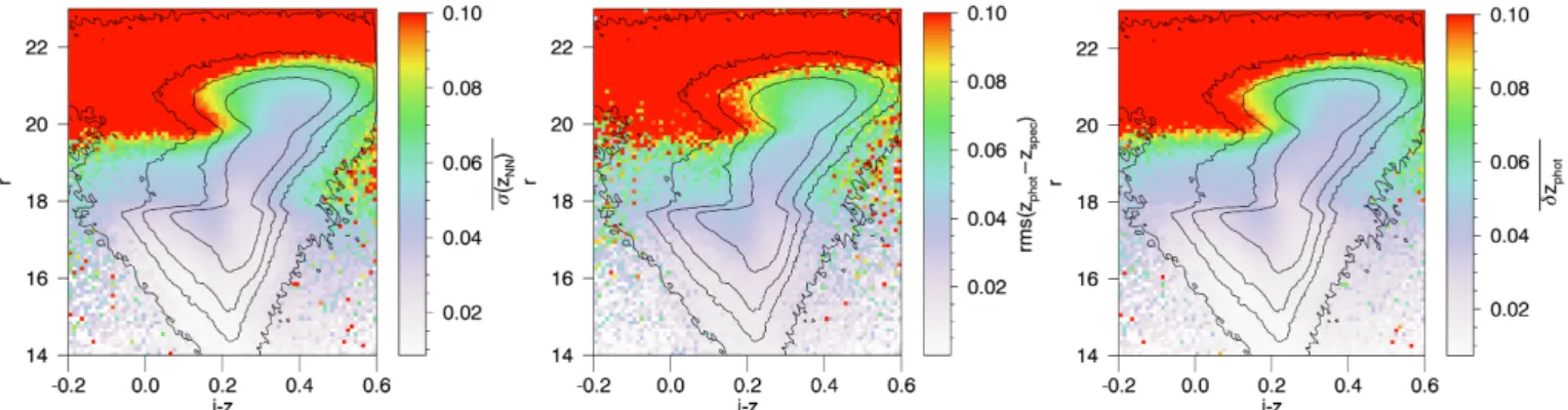
Figure6illustrates this effect in the g−r and r−i colour plane. The colour maps in this figure show three measurements of the redshift estimation error as a function of g − r and r − i: the aver-age standard deviation of the redshifts of the nearest neighbours σ(zNN), the root mean square (rms) of the actual error zphot−zspec,
and the average estimated errors δzphot. The different error
mea-surements show a similar behaviour. The estimated error δzphot is
closely related to the actual error, which further supports that it is a good estimator of the error, as previously shown in Fig.5. As expected, both errors are clearly correlated with the deviation of the redshifts of the nearest neighbours. In the regions where the dispersion is higher, the redshift estimation has a bigger error. The contour lines in Fig.6represent the galaxy count distribu-tion of the training set T5. By comparing these contours with the
background error maps, we see that there is a clear correlation between the photometric redshift errors and the galaxy count dis-tribution: denser regions yield smaller errors and sparser regions yield bigger errors.
Figure7shows the same three measurements of the redshift estimation error shown in Fig.6as a function of r and i − z. The behaviour is similar to that observed in Fig.6, with an estimated error δzphot closely following the deviation of the redshifts of the
nearest neighbours σ(zNN) and the actual error zphot− zspec. The
contour lines in this figure show the galaxy count distribution as a function of r and i − z. By comparing these contours with the error maps, we again see a correlation between the two, although less clear than in Fig.6. This is due to an additional effect that is analysed in the next part: fainter galaxies tend to have larger errors than brighter galaxies.
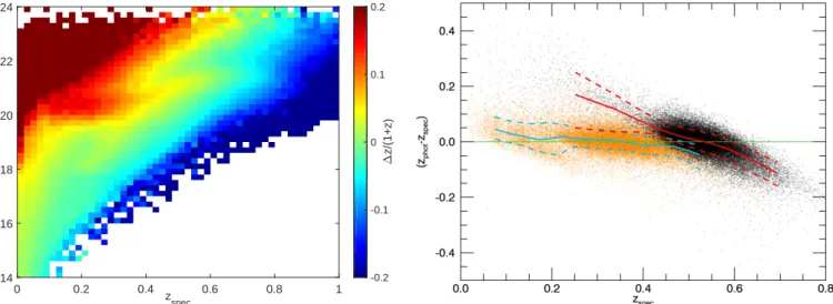
In fact, one of the input features of the proposed method depends directly on the r-band magnitude of the galaxies, and thus, on their apparent brightness. This feature has a strong impact on the estimation of the photometric redshift, as shown in Fig. 8. The left panel of Fig.8shows the average normalised
Fig. 6.Photometric redshift results as a function of the r − i and g − r colours. These results were obtained with a 100-fold cross-validation strategy on the set of galaxies with the five magnitudes available (T5). Left panel: average standard deviation of the redshifts of the nearest neighbours
σ(zNN), middle panel: rms of the actual error zphot− zspec, and right panel: average estimated errors δzphot. For easier comparison, the scale in the
three panels was set between 0 and 0.1, with red indicating errors that are bigger than or equal to 0.1. For reference, the black lines represent the contours of the galaxy count distribution of the training set T5, with the four displayed contours corresponding to 1000, 300, 100, and 10 galaxies
per colour bin.
Fig. 7.Photometric redshift results as a function of the r magnitude and the i−z colour. These results were obtained with a 100-fold cross-validation strategy on the galaxy set with the five magnitudes available (T5). Left panel: average standard deviation of the redshifts of the nearest neighbours
σ(zNN), middle panel: rms of the actual error zphot− zspec, and right panel: average estimated errors δzphot. The colour scale and the black contours
are set as in Fig.6.
error∆znorm= (zphot− zspec)/(1+ zspec) as a function of the
mag-nitude r and the spectroscopic redshift zspec. While for brighter
galaxies (r < 20) the average normalised error is below 0.1, for fainter galaxies (r > 20) the error increases significantly, espe-cially for galaxies at z < 0.4 or z > 0.8. The right panel of Fig.8shows the redshift error zphot−zspecfor bright (18 < r < 20)
and faint (20 < r < 21) galaxies. While the redshift of brighter galaxies is well estimated, with a small bias both at low and high redshift, the error for fainter galaxies is higher, especially when the true redshift is far from 0.5−0.6.
4.4. Impact of missing features
The proposed approach is also able to work when one or several features are missing. When this occurs, the performance of the method degrades, with an increased scatter in the photometric versus spectroscopic redshift relation. Missing features usually appear in very faint galaxies, but can also occur in brighter galax-ies due to photometric measurement errors. In our training set T with 2 313 724 galaxies, the r Kron magnitude is missing from 48 416 galaxies (2.1%), and the g − r, r − i, i − z and z − y aperture colours are missing from 144 352 (6.2%), 51 150 (2.2%), 52 357 (2.3%), and 57 350 (2.5%) galaxies, respectively. Most of these galaxies are faint. For example, approximately 91% of the galax-ies without the g − r aperture colour have an r Kron magnitude r> 20, while only 9% are brighter than r = 20.
To evaluate the effect of a missing feature independently of the position of the galaxy in the magnitude-colour space, we artificially removed one of the features from our training set T5, and repeated the experiment described in Sect. 4.1, using
the four remaining features for both the test and training sub-sets. The results are similar to those presented in Fig. 4, but with a higher scatter. Table 5 summarises the results obtained when the different features are removed. When the r Kron mag-nitude is removed, the standard deviation of the normalised bias is σ(∆znorm)= 0.0364, 22% higher than when using the five
fea-tures (σ(∆znorm) = 0.0299). The effect is smaller when one of
the aperture colours is removed, with an increase of 13%, 11%, 4%, and 1% in σ(∆znorm) for g − r, r − i, i − z, and z − y,
respec-tively. This indicates that, among the five features, the r Kron magnitude has the strongest effect in the determination of the photometric redshifts, while the aperture colours play a weaker role. On the other hand, the average bias remains small, and the outlier rate is not affected much by the removal of any of the colour features, but increases when the r magnitude is removed.
5. Comparison with other photometric features The photometric redshift estimation method described in Sect.2 is a general technique that can be applied to different sets of fea-tures. In the previous section, we presented the results obtained when using the five PS1 features described in Sect.2.2, meaning
0 0.2 0.4 0.6 0.8 1 z spec 14 16 18 20 22 24 r -0.2 -0.1 0 0.1 0.2 z/(1+z)
Fig. 8.Left panel: average normalised error∆znorm= (zphot− zspec)/(1+ zspec) as a function of the magnitude r and the spectroscopic redshift zspec.
Right panel: redshift error zphot− zspecas a function of the spectroscopic redshift zspecfor galaxies with 18 < r < 20 (orange dots) and 20 < r < 21
(black dots). Each dot represents an individual galaxy (only 10% of the galaxies are shown, for better visualisation). The thick solid and dotted lines represent the median and the 68% confidence regions, respectively, computed in small zspecintervals for the galaxies with 18 < r < 20 (blue
lines) and 20 < r < 21 (red lines). The green line shows zphot = zspec. The results in both panels were obtained with a 100-fold cross-validation
strategy on T5.
Table 5. Average normalised redshift estimation bias∆znorm, standard
deviation σ(∆znorm) and outlier rate Po for the experiments in which
one of the features is removed.
Removed feature ∆znorm σ(∆znorm) Po
r 1.03 × 10⁻³ 0.0364 5.62
g − r −2.97 × 10⁻⁴ 0.0340 4.01
r − i −1.12 × 10⁻³ 0.0330 4.39
i − z −1.85 × 10⁻⁴ 0.0310 4.11
z −y −2.44 × 10⁻⁴ 0.0302 4.18
Notes. These quantities were calculated after iteratively removing the outliers, defined as |∆znorm|> 3σ(∆znorm).
the PS1 r-band Kron magnitude and the g − r, r − i, i − z, and z − y aperture colours. In this section, we analyse the effects of using different sets of features. In particular, we consider two differ-ent cases: (1) PS1 Kron colours, and (2) SDSS features, as in Beck et al.(2016). In the first case, we assess whether the Kron colours, which are not physically motivated (see Sect. 2.2) but directly available for download for the complete PS1 survey, can be used if more convenient. Considering the SDSS features will allow us to compare the performance of the method using PS1 information with respect to the original method ofBeck et al. (2016).
In order to make a fair comparison, we restricted our training set to the galaxies in T that have the r-band Kron magnitude, the four aperture colours, and the four Kron colours available in the PS1 dataset. Moreover, we also discard the galaxies that do not satisfy the colour cut and photometric error criteria defined in Eq. (7) ofBeck et al.(2016), based on SDSS information. The resulting training set, TBeck
9 , contains 1 776 508 galaxies. As in
the previous experiments described in Sect. 4, we performed a 100-fold cross-validation to evaluate the performance, but using TBeck
9 instead of T5. We computed the photometric redshift of
the galaxies in the 100 test sets using: (1) the r-band Kron mag-nitude and the four aperture colours from PS1; (2) the r-band
Table 6. Average normalised redshift estimation bias∆znorm, standard
deviation σ(∆znorm), and outlier rate Poobtained when using different
sets of features in the training set TBeck 9 .
Features ∆znorm σ(∆znorm) Po
PS1 aperture colours −3.97 × 10⁻⁵ 0.0279 3.15
PS1 Kron colours 1.24 × 10⁻⁴ 0.0283 3.10
SDSS −2.02 × 10⁻⁴ 0.0197 3.82
Notes. These quantities were calculated after iteratively removing the outliers, defined as |∆znorm|> 3σ(∆znorm).
Kron magnitude and the four Kron colours from PS1; and (3) the five SDSS features defined inBeck et al.(2016) as features.
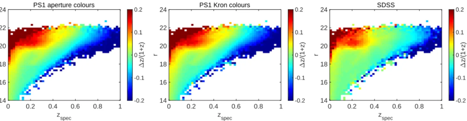
Table6reports the average bias, standard deviation, and out-lier rate obtained in the three cases. Figure9shows the average normalised bias in the three cases as a function of the r-band Kron magnitude and the spectroscopic redshift zspec. The results
obtained with PS1 aperture colours are not exactly the same as in the experiment presented in Sect.4(see Table4and Fig.8) because the training set (TBeck
9 instead of T5) now contains fewer
galaxies. The galaxies that were removed with respect to T5are
those for which a PS1 Kron magnitude is missing or that do not satisfy the SDSS criteria defined in Beck et al. (2016). These are probably galaxies with poorer photometry, which explains the slight improvement in the performance (lower standard devi-ation and outlier rate) with respect to the results presented in Sect.4.
5.1. Aperture colours versus Kron colours
As shown in Table 6 and Fig. 9, the results obtained when using Kron colours are very similar to the ones obtained when using aperture colours. We also saw a nearly identical perfor-mance to the one shown in Figs.4and5: the photometric red-shift calculated from Kron colours follows the spectroscopic redshift quite well, especially in the intermediate redshift range
PS1 aperture colours 0 0.2 0.4 0.6 0.8 1 zspec 14 16 18 20 22 24 r -0.2 -0.1 0 0.1 0.2 z/(1+z) PS1 Kron colours 0 0.2 0.4 0.6 0.8 1 zspec 14 16 18 20 22 24 r -0.2 -0.1 0 0.1 0.2 z/(1+z) SDSS 0 0.2 0.4 0.6 0.8 1 zspec 14 16 18 20 22 24 r -0.2 -0.1 0 0.1 0.2 z/(1+z)
Fig. 9.Average normalised error∆znorm = (zphot− zspec)/(1+ zspec) as a function of the magnitude r and the spectroscopic redshift zspec, for three
different sets of features: left panel: PS1 features with aperture colours; middle panel: PS1 features with Kron colours; and right panel: SDSS features. In the three cases, the results were obtained with a 100-fold cross-validation strategy on TBeck
9 .
Fig. 10.Correlation between the r − i colour and the spectroscopic redshift zspecfor SDSS (left panel) and PS1 (right panel) datasets. In the PS1
case, the aperture colour is represented. Each point represents a galaxy of the training set TBeck 9 .
(0.1 < zspec < 0.6), and the method tends to underestimate the
redshift for high-redshift galaxies (zspec > 0.6) and to
overesti-mate it for low-redshift galaxies (zspec< 0.1).
Since the difference between using PS1 aperture colours or PS1 Kron colours is negligible, we have included the possibil-ity of selecting which features to use in the code available at the project website. The user may choose the one that is more con-venient, without significant impact on the results.
5.2. PS1 features versus SDSS features
Figure9and Table6show that using SDSS information instead of PS1 information results in a slightly better performance. The standard deviation of the normalised redshift error is lower with SDSS features. Moreover, although the global average bias is smaller for PS1 (with aperture colours), Fig. 9 shows that SDSS features result in a lower bias both at high and low redshift. This effect is especially noticeable for fainter galax-ies. In the following, we analyse the possible causes of this behaviour.
Firstly, PS1 and SDSS features are defined differently. One of the SDSS features is the u − g colour, which is not available in PS1; whereas the z − y colour is available in PS1 but not in SDSS. Including a bluer information in SDSS allows a better estimation of the redshift of lower redshift galaxies. To check if
this is enough to explain the observed behaviour, we repeated the calculation of the photometric redshift removing the u − g colour from SDSS features and removing the z − y colour from PS1 fea-tures. The results with SDSS features degrade, but still show a slightly better performance than with PS1 features, so this fea-ture difference does not entirely explain the better behaviour of SDSS features.
Secondly, the magnitudes g, r, i, and z have different values in SDSS and PS1. It turns out that SDSS magnitudes show a better correlation with the spectroscopic redshift, which explains their power to better estimate the photometric redshift. Figure10 shows a comparison of the correlation between the r − i colour and the spectroscopic redshift for SDSS and PS1 (considering the r − i aperture colour). For a given redshift, PS1 values show a larger dispersion than SDSS. The same occurs for the g − r and i − zaperture colours, for the Kron colours, and for the r Kron magnitude. The reason for this larger scatter could be that PS1 aperture colours are not measured exactly at the Kron radius, but at the closest one from the five available apertures, resulting in colours that do not correspond to the same percentage of flux for all the galaxies. Conversely, SDSS colours are computed from ModelMag magnitudes, so they correspond to the total flux of the galaxy. On the other hand, PS1 Kron colours are not physically motivated, since they are calculated as the difference between two magnitudes that may be measured in different radii.
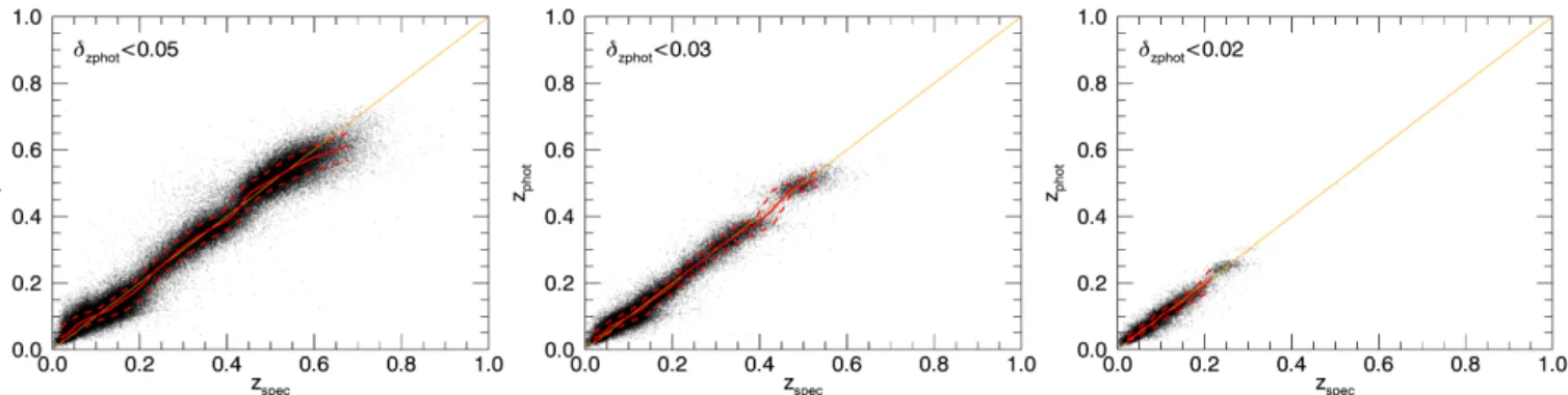
Fig. 11.Photometric redshift as a function of spectroscopic redshift for three different sets. The red solid and dashed lines represent the median
and the 68% confidence regions, respectively, computed at small zspecintervals. The orange line shows zphot = zspec. On panel a, we included the
galaxies with a reported redshift error of δzphot < 0.05. On panel b, we included the galaxies with a reported redshift error of δzphot < 0.03. On panel
c, we included the galaxies with a reported redshift error of δzphot< 0.02. Only 10% of the galaxies are shown, for better visualisation.
Fig. 12.Photometric redshift as a function of spectroscopic redshift, for three different sets. The red solid and dashed lines represent the median and the 68% confidence regions, respectively, computed in small zspecintervals. The orange line shows zphot= zspec. On panel a, we included the
galaxies in photometric error Class 1 and with a reported redshift error of δzphot < 0.05. On panel b, we included the galaxies in photometric error
Class 1 and with a reported redshift error of δzphot < 0.03. On panel c, we included the galaxies in photometric error Class 1 and with a reported
redshift error of δzphot< 0.02. Only 10% of the galaxies are shown, for better visualisation.
6. Practical guidelines for using the method
The training set T and the code implementing our approach are available for download at the project website. This allows the estimation of the photometric redshift of any galaxy in the PS1 survey. The code includes several configuration options that are described in detail in the webpage. The two main options are the choice between aperture or Kron magnitudes, and the choice of the subset of T to be used for training.
Depending on the required accuracy and on the specific use of the photometric redshifts provided by our approach, one may want to use all the possible photometric redshifts regardless of their error, or prefer to use a lower amount of more accurate pho-tometric redshifts. In this section, we present different options to select the best redshifts.
There are three main parameters that can be used for this selection: the estimated error δzphot, the photometric error class,
and the extrapolation flag. Figure11shows the effect of using different cuts in the photometric redshift errors. As expected, introducing a cut in δzphot reduces the errors (see for
compari-son Fig.4, where no cuts were used). However, if the cut is too severe, the resulting sample may be limited in terms of redshift and colour space coverage. Therefore, we suggest testing di ffer-ent values to find the most appropriate one for a particular goal. Figure12shows the effect of adding a cut using the photomet-ric error class. By comparing Figs.11and12, we can see that the photometric error class selection mainly reduces the scatter at high redshifts, where the photometric errors are larger.
Given the low number of galaxies in our dataset for which an extrapolation was performed, filtering them out does not bring a noticeable effect overall. However, this parameter is a good indicator of the accuracy of the results, as shown in Table4, so it can be used to filter out some of the calculated redshifts when there is a need for high accuracy.
Finally, the error maps presented in Sect. 4.3can be used to filter out some of the galaxies located in the regions of the magnitude-colour space that are more prone to errors.
Since we provide the training set and the redshift estimation code separately, the user may modify the training set by adding additional galaxies according to his/her needs. Additionally, our training set can be used as well with different data-driven red-shift estimation algorithms (neural networks, decision trees, etc). A comparison of the performance using different algorithms is beyond the scope of this paper, but we checked that the proposed approach provides very similar results to the ones obtained with PhotoRaptor (Cavuoti et al. 2016) and a 100-trees random for-est from scikit-learn (Pedregosa et al. 2011). It is worth noting, however, that our approach has the advantages of providing an estimation of the photometric redshift error and being less com-putationally complex.
7. Summary
We present a data-driven approach to compute photometric red-shifts for galaxies using the PS1 survey. In this work, we used data from the PS1 DR2, but we tested the results also for the
DR1, finding no significant difference. Our approach is an appli-cation of the method proposed by Beck et al. (2016) for the SDSS DR12, based on a local linear regression in a 5D magni-tude and colour space. To apply theBeck et al.(2016) algorithm to PS1, we selected appropriate magnitudes and colours (r, g − r, r − i, i − z, and z − y) to define the 5D space, and we constructed a proper and clean training set composed of 2 313 724 galaxies, of which the spectroscopic redshift is available from SDSS and the magnitudes and colours were obtained from the PS1 DR2 survey. A version of the code and training set is available for download at the project website.
We assessed the performance of this approach by means of a cross-validation on the training set, meaning we used part of the galaxies of our training set as test galaxies to estimate their photometric redshifts, and we then compared them to their true (spectroscopic) redshifts. We estimate that the average bias of our approach is ∆znorm = −1.92 × 10⁻⁴, its standard deviation,
σ(∆znorm)= 0.0299, and the outlier rate Po= 4.30%.
We also evaluated the impact of the photometric uncertain-ties on our redshift determination. This was done by dividing the entire sample in five photometric classes of growing photo-metric errors. As expected, the uncertainties on the photophoto-metric redshifts are smaller where the photometric errors are smaller. There is also a fraction of galaxies for which the method extrap-olates the photometric redshift, since their features lie outside the bounding box of their nearest neighbours. In these cases, the errors on photometric redshifts are larger and these galaxies are flagged appropriately.
Moreover, we analysed the impact of the galaxy density (in the feature space) on the redshift determination. In fact, there are regions in the 5D space that are more populated than others. As expected, we find that galaxies located in crowded regions have a better redshift estimation than galaxies found in sparse regions. Since galaxies in PS1 may have incomplete photometry, our approach is prepared to deal with the case of missing features. We evaluated the effect that a missing feature may produce on the results using an ablation test (artificially removing existing features). As expected, the scatter increases in these cases. This effect is especially important when the r Kron magnitude is miss-ing, whereas a missing colour has a smaller impact.
Furthermore, we tested the use of PS1 Kron colours instead of aperture colours, finding no significant difference in the results. Although Kron colours have no physical meaning, they are easier to obtain, and it is worth stressing that they can be safely used for computing photometric redshifts with our approach.
Finally, we compared our results with those presented in Beck et al.(2016) for the SDSS DR12. We find that SDSS data perform slightly better than PS1 features, especially for faint galaxies (r > 20). We suggest that these differences could be caused by two main factors: different available filters, with SDSS offering a bluer band, and a stronger correlation between the SDSS magnitudes and the spectroscopic redshift. However, it is worth noting that the overall performance of our approach is fully in agreement (within the uncertainties) with the SDSS results.
Acknowledgements. The research leading to these results has received
fund-ing from the European Research Council under the European Union’s
Sev-enth Framework Programme (FP7/2007–2013)/ERC grant agreement n◦340519.
The authors would like to thank Monique Arnaud for helpful discussions and
suggestions. This research has made use of the STARRS1 Survey. The Pan-STARRS1 Surveys (PS1) and the PS1 public science archive have been made possible through contributions by the Institute for Astronomy, the University of Hawaii, the Pan-STARRS Project Office, the Max-Planck Society and its partic-ipating institutes, the Max Planck Institute for Astronomy, Heidelberg and the Max Planck Institute for Extraterrestrial Physics, Garching, The Johns Hopkins University, Durham University, the University of Edinburgh, the Queen’s University Belfast, the Harvard-Smithsonian Center for Astrophysics, the Las Cumbres Observatory Global Telescope Network Incorporated, the National Central University of Taiwan, the Space Telescope Science Institute, the National Aeronautics and Space Administration under Grant No. NNX08AR22G issued through the Planetary Science Division of the NASA Science Mission Direc-torate, the National Science Foundation Grant No. AST-1238877, the Univer-sity of Maryland, Eotvos Lorand UniverUniver-sity (ELTE), the Los Alamos National Laboratory, and the Gordon and Betty Moore Foundation. This research has also made use of the SDSS-III Survey (DR12). Funding for SDSS-III has been provided by the Alfred P. Sloan Foundation, the Participating Institutions, the
National Science Foundation, and the US Department of Energy Office of
Sci-ence. The SDSS-III web site ishttp://www.sdss3.org/. Some of the data
presented in this paper were obtained from the Mikulski Archive for Space Telescopes (MAST). STScI is operated by the Association of Universities for Research in Astronomy, Inc., under NASA contract NAS5-26555. Support for MAST for non-HST data is provided by the NASA Office of Space Sci-ence via grant NNX13AC07G and by other grants and contracts. The authors acknowledge the use of the Catalog Archive Server Jobs System (CasJobs)
ser-vice athttp://casjobs.sdss.org/CasJobs, developed by the JHU/SDSS
team.
References
Ahumada, T., Anand, S., Andreoni, I., et al. 2020,GRB Coordinates Netw.,
27737, 1
Alam, S., Albareti, F. D., Allende Prieto, C., et al. 2015,ApJS, 219, 12
Almosallam, I. A., Jarvis, M. J., & Roberts, S. J. 2016,MNRAS, 462, 726
Beck, R., Dobos, L., Budavári, T., Szalay, A. S., & Csabai, I. 2016,MNRAS, 460, 1371
Benítez, N. 2000,ApJ, 536, 571
Bolzonella, M., Miralles, J. M., & Pelló, R. 2000,A&A, 363, 476
Brammer, G. B., van Dokkum, P. G., & Coppi, P. 2008,ApJ, 686, 1503
Carrasco Kind, M., & Brunner, R. J. 2013,MNRAS, 432, 1483
Cavuoti, S., Brescia, M., De Stefano, V., & Longo, G. 2016, ArXiv e-prints
[arXiv:1602.05408]
Cavuoti, S., Amaro, V., Brescia, M., et al. 2017,MNRAS, 465, 1959
Chambers, K. C., Magnier, E. A., Metcalfe, N., et al. 2016, ArXiv e-prints
[arXiv:1612.05560]
Collister, A. A., & Lahav, O. 2004,PASP, 116, 345
Csabai, I., Dobos, L., Trencséni, M., et al. 2007,Astron. Nachr., 328, 852
Dark Energy Survey Collaboration (Abbott, T. et al.) 2016,MNRAS, 460, 1270
Fitzpatrick, E. L. 1999,PASP, 111, 63
Flewelling, H. A., Magnier, E. A., Chambers, K. C., et al. 2019, ArXiv e-prints
[arXiv:1612.05243]
Goto, T., Okamura, S., McKay, T. A., et al. 2002,PASJ, 54, 515
Graham, M. L., Connolly, A. J., Ivezi´c, Ž., et al. 2018,AJ, 155, 1
Hennawi, J. F., Myers, A. D., Shen, Y., et al. 2010,ApJ, 719, 1672
Ilbert, O., Arnouts, S., McCracken, H. J., et al. 2006,A&A, 457, 841
Magnier, E. A., Chambers, K. C., Flewelling, H. A., et al. 2019, ArXiv e-prints
[arXiv:1612.05240]
Pedregosa, F., Varoquaux, G., Gramfort, A., et al. 2011,J. Mach. Learn. Res., 12, 2825
Reusch, S., Stein, R., & Franckowiak, A. 2020,GRB Coordinates Netw., 28005, 1
Rodney, S. A., & Tonry, J. L. 2010,ApJ, 723, 47
Ross, A. J., Percival, W. J., & Brunner, R. J. 2010,MNRAS, 407, 420
Sadeh, I., Abdalla, F. B., & Lahav, O. 2016,PASP, 128, 104502
Saglia, R. P., Tonry, J. L., Bender, R., et al. 2012,ApJ, 746, 128
Salvato, M., Ilbert, O., & Hoyle, B. 2019,Nat. Astron., 3, 212
Schlegel, D. J., Finkbeiner, D. P., & Davis, M. 1998,ApJ, 500, 525
Speller, R., & Taylor, J. E. 2014,ApJ, 788, 188
Stoughton, C., Lupton, R. H., Bernardi, M., et al. 2002,AJ, 123, 485
Streblyanska, A., Barrena, R., Rubiño-Martín, J. A., et al. 2018,A&A, 617, A71
Tarrío, P., Melin, J. B., & Arnaud, M. 2019,A&A, 626, A7
Tonry, J. L., Stubbs, C. W., Lykke, K. R., et al. 2012,ApJ, 750, 99