An Ising model for earthquake dynamics

HAL Id: hal-00302814

https://hal.archives-ouvertes.fr/hal-00302814

Submitted on 19 Jan 2007

HAL is a multi-disciplinary open access

archive for the deposit and dissemination of

sci-entific research documents, whether they are

pub-lished or not. The documents may come from

teaching and research institutions in France or

abroad, or from public or private research centers.

L’archive ouverte pluridisciplinaire HAL, est

destinée au dépôt et à la diffusion de documents

scientifiques de niveau recherche, publiés ou non,

émanant des établissements d’enseignement et de

recherche français ou étrangers, des laboratoires

publics ou privés.

A. Jiménez, K. F. Tiampo, A. M. Posadas

To cite this version:

A. Jiménez, K. F. Tiampo, A. M. Posadas. An Ising model for earthquake dynamics. Nonlinear

Processes in Geophysics, European Geosciences Union (EGU), 2007, 14 (1), pp.5-15. �hal-00302814�

© Author(s) 2007. This work is licensed

under a Creative Commons License.

in Geophysics

An Ising model for earthquake dynamics

1_{Department of Earth Sciences Biological and Geological Sciences, University of Western Ontario, London, Canada} 2_{Department of Applied Physics, University of Almer´ıa, Spain}

Received: 2 November 2006 – Revised: 19 December 2006 – Accepted: 22 December 2006 – Published: 19 January 2007

Abstract. This paper focuses on extracting the information contained in seismic space-time patterns and their dynamics. The Greek catalog recorded from 1901 to 1999 is analyzed. An Ising Cellular Automata representation technique is de-veloped to reconstruct the history of these patterns. We find that there is strong correlation in the region, and that small earthquakes are very important to the stress transfers. Fi-nally, it is demonstrated that this approach is useful for seis-mic hazard assessment and intermediate-range earthquake forecasting.

1 Introduction

Earthquake faults occur in topologically complex, multi-scale networks or systems that are driven to failure by ex-ternal forces arising from plate tectonic motions. The ba-sic problem is that the details of the true space-time, force-displacement dynamics are unobservable, in general. How-ever, the space-time patterns associated with the time, lo-cation, and magnitude of the sudden events (earthquakes) are observable, leading to a focus on understanding their observable, multi-scale, apparent dynamics (Rundle et al., 2003). Regional seismicity has many characteristics of a crit-ical system (Hirata, 1989; Hirata and Imoto, 1991; Smalley et al., 1987; Omori, 1895; Bufe and Varnes, 1993; Sammis and Smith, 1999; Bowman and King, 2001). The observed scaling laws associated with earthquakes, and its large-scale correlations, have led a variety of researchers to the conclu-sion that these events can be regarded as a type of general-ized phase transition, similar to the nucleation and critical phenomena that are observed in thermal and magnetic sys-tems (Rundle et al., 2003). As a result, many investigators have explored the possibility of using formalisms from sta-Correspondence to: A. Jim´enez

(ajimene@uwo.ca)

tistical physics to model the spatial, temporal and magnitude distributions (All`egre et al., 1982; All`egre and Le Mouel, 1994; Rundle, 1993; Sornette and Sornette, 1989; Sornette and Sammis, 1995; Tiampo et al., 2002b,a). This statistical physics approach differs from the earlier approaches by its emphasis on the treatment of earthquake faults and fault sys-tems as high-dimensional dynamical syssys-tems characterized by a wide range of scales in both space and time.

Phase transitions are observed in surprisingly simple sys-tems, e.g. on a lattice of interacting spins. The Ising model was proposed by Wilhelm Lenz (1888–1957) in 1920 for studying some ferromagnetic properties. It was solved ex-actly for the one-dimensional case by his student Ernest Ising in 1925. Lars Onsager solved the Ising model in 1944 for two dimensions in the absence of an external magnetic field and showed that there was a phase transition in two dimen-sions. The two-dimensional Ising model is the simplest non-trivial model of a phase transition (Gould and Tobochnik, 2004). The model imitates situations where individual ele-ments (atoms, animals, proteins, biological cells, social be-havior, etc.) modify their behavior so that they mimic their neighbors’ behavior. It has been used for modeling phase transitions in binary alloys (Kroll and Gompper, 1987) and spin glasses (Boettcher and Hartmann, 2005). In biology, it can model neural networks (Schaap, 2005), bird flocks (Colella et al., 2001) or heart cell beats (Wong, 2005). In ad-dition, it has been applied to sociology or seismology (Tou-ssaint and Pride, 2004). More than 12 000 papers have been published between 1969 and 1997 that use the Ising model to model complex behaviors resulting from simple neighbor-hood interactions.

Jim´enez et al. (2005); Jim´enez and Posadas (2006) de-veloped a method based on Cellular Automata, where the activity in the cell is explicitly given by the activity in the same cell and in its neighbors in the past. The state of the neighborhood is given by the added surrounding activity, so that activity triggers activity. However, no quiescence was

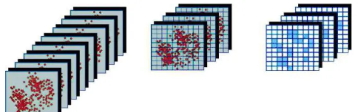
Fig. 1. Coarse-graining of the data set.

introduced, so that an inactive cell has no interaction with its neighbors. In the present paper we will introduce an Ising model scheme, so that this “inactivity” is taking into account.

2 The model 2.1 The Ising model

In the Ising model, the spin at every site is either up (+1) or down (−1). Unless otherwise stated, the interaction is between nearest neighbors only and is given by −J if the spin are parallel and +J if the spins are anti-parallel. The total energy can be expressed in the form:

E = −JX i,j SiSj−B X i Si (1)

where Si=±1, J is known as the exchange constant and B is the external (magnetic) field. In a Cellular Automata rep-resentation, the energy is calculated for each site, j being the nearest neighbors, and added. The spin-flip probability is given by the Boltzmann probability function.

P (E) = 1 Zexp(−

E

kT) (2)

where P (E) is the probability of finding the system in the state of energy E, T is the temperature, k is the Boltzmann constant and Z is the partition function. The algorithm for simulating it is that of Metropolis: at a the first step, a grid with n cells with initial state (+1) or (−1) is created. Then, a loop starts: i) a cell is randomly chosen; ii) the spin-flip p probability is the minimum between 1 and exp(−1E_kT ), where 1E is given by Eq. (1), and represents the energy change if

a cell exchanges its state (if the exchange is favored or not); iii) a random number is calculated, between 0 and 1 and, if it is lower than p, the state of the cell is changed; iv) another cell is randomly chosen, and the procedure goes on. The basic unit of time is the Monte Carlo step, which equals n2 trials of spin-flip, so that all the cells have the opportunity of changing in average.

The order parameter for a magnetic system is the mag-netization. In this model, it is calculated as the difference between spins with state up and spins with state down. The parameter which controls the state of the system is the tem-perature. At equilibrium, for low temperatures the system is

ordered, and all the spins are up or down. When the temper-ature is high, the system is disordered, and the magnetization is null. There is a critical temperature, when the magneti-zation is null, but the system is ordered in clusters, and rep-resents the transition from an ordered phase to a disordered one.

This type of model, as are those derived from the Burridge and Knopoff (1967) model, is a direct one, where the initial conditions are given, as well as the transition rules (which depends on the control parameter), and it is iterated several times for analyzing its behavior. The parameters of inter-est (magnetization, for example) are calculated as averages (macroscopic magnitudes), and the particular state of the cell in each time is not important, but the properties of the whole system are of interest. They have been used to successfully describe the macroscopic behavior of the seismicity, such as the Gutenberg-Richter law, the temporal and spatial cluster-ing of the hypocenters (Carlson and Langer, 1989b,a; Chris-tensen and Olami, 1992; Nakanishi, 1990, 1991; Olami et al., 1992; Otsuka, 1972; Bak and Tang, 1989; Bak et al., 1988; Barriere and Turcotte, 1991; Rundle, 1988; Rundle et al., 2002; Anghel et al., 2000; Klein et al., 1997, 2000). Here, we are interested in the inverse problem. Given a particular pattern series, we wish to calculate its transition rules. Note that the Metropolis algorithm has a random component and, for the same initial configuration, the successive steps in two different realizations will be different as well, but the station-ary state for the macroscopic magnitudes will be the same. The particular history is not important. In the present work, however, we are precisely interested in the particular history of the patterns.

2.2 Method

The pattern series can be modeled in terms of a Cellular Au-tomaton where the transition rules are calculated by means of the maximization of the mutual information (Jim´enez et al., 2005; Jim´enez and Posadas, 2006), and the particular pat-terns’ history is successfully emulated. In that case, the avail-able states were 0 or 1 only, and the transition rules (the state of the cell given a particular neighborhood’s state) were given by the number of neighboring active cells (Hirata and Imoto, 1997). Here, we transform this scheme for using the Ising model: first of all, the available states are (+1) for an active cell and (−1) for an inactive one (quiescent). Then, we can define the state of the neighborhood by means of the energy levels calculated with Eq. (1).

We now consider whether a Cellular Automaton which reproduces the seismic activity in a region following an Ising interaction scheme can be constructed. After a coarse-graining of the events, both spatially and temporally, a state (active or quiescent for seismic activity) is assigned to each cell at each time step (Fig. 1). The activation criteria are based on the time series given by the expression:

ǫq(N (τ )) = N (τ )_X

n=1

εnq (3)

where εnis the released energy of the nt hevent, and N (τ ) is the number of earthquakes in a given interval of time τ , and where the energy is calculated from the relationship between magnitude and energy (Gutenberg and Richter, 1956). When

q=1, ǫq represents the accumulated energy; with q=1/2, is the quantity known as Benioff strain (Sammis and Smith, 1999); for q=1/3, it is an approximation of the fault slip dimension (Mai and Beroza, 2000; Carpinteri and Pugno, 2005); and for q=0 it is simply the number of the events. With q<1 in Eq. (3) the effect is that of smoothing the en-ergy, acting as a low pass filter (Jim´enez et al., 2006).

Thus, the activation criteria follows the scheme: if the cu-mulative ǫq from Eq. (3) in a cell at each interval of time is greater or equal than an established threshold (equivalent to a certain magnitude, m, related to the q root of the energy re-lease), the cell is considered active (+1) and, otherwise, qui-escent (−1). Since this energy threshold is arbitrary, differ-ent energies (magnitudes) are analyzed. However, for q=0 we can not distinguish between different magnitudes. In this case, a cell is considered active if ǫqis greater or equal than the mean value divided by the standard deviation at that inter-val of time (α1criterion). This choice gives us an estimation

of the behavior of the fluctuations of the considered quan-tity. Furthermore, we can also use the values for comparing the activity with the mean divided by the standard deviation of the entire interval of time (α2criterion), for a mean field

approximation.

A serial of lattice configurations (patterns) is obtained. As-suming that each cell interacts only with its nearest neigh-bors, we can calculate the transition rules directly from these patterns (Jim´enez et al., 2005), by means of a histogram of occurrences. However, the predictive capacity of the model depends on the number of cells, N, and time interval, t, cho-sen. By maximizing the mutual information, µI, between the past and future states we can find the model which contains a higher correlation between them (Cover and Thomas, 1991). The expression for µIin this particular model is as follows:

µI = 1 X i=0 1 X j =0 En X k=E0 p(i; j, k) lg₂ p(i; j, k) p(i)p(j, k) (4)

with p(i; j, k) being the joint probability of past and future states, and p(i)p(j, k) a distribution of independent states,

(i) stands for the central cell at time t+τ , and (j, k) is for

the central and its k “neighborhood’s state” at time t, with Ei (i∈[0, n], i∈N ) representing the possible states. The calcu-lated µI value represents the expected value of the “informa-tion gain” by using a model with interacting cells instead of another model where the consecutive states are independent (Daley and Vere-Jones, 2004). To find the maximum, a grid

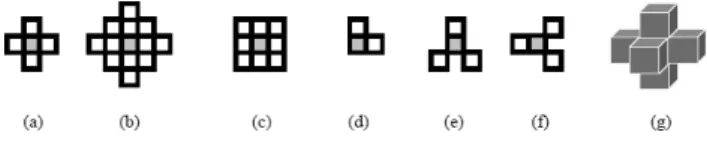
Fig. 2. Some neighborhoods.

search in time steps and number of cells is made and, finally, we derive our Cellular Automaton.

Once we have the Cellular Automaton, we can test how well it reproduces the data. First, the transition rules are applied to each real pattern, and an activation probability is obtained for each cell. Then, the cells are declared active or inactive using these probabilities (Posadas et al., 2000). Once the real and simulated patterns for each time are ob-tained, the correlation function (Vicsek, 1992) and the Ham-ming distance (Ryan and Frater, 2002) are used to compare them. The latter is simply the number of cells that failed in the prediction, representing the simulation error. If the Cel-lular Automaton rules are applied to the latest pattern, we ob-tain what we call a Probabilistic Activation Map, where the probability of surpassing certain cumulative ǫq (equivalent to certain magnitude), or being more active than the average (q=0) in the next interval of time is shown (Jim´enez et al., 2005; Jim´enez and Posadas, 2006).

In an Ising model, as explained, the flip transitions are given by the energy state of the cells, so that a cell in a state has a certain probability of changing it depending on the energy of the interactions with its neighborhood and the external field. In our method, these probabilities have to be calculated, since we assume that we have no a priori hypoth-esis about the nature of the interactions between neighboring sites, nor between the sites and an external field. Therefore, we classify the neighborhoods configuration in terms of its “energetic” state, so that each cell has an associated energy given by Eq. (1), with Si the central cell’s state and Sj is the neighboring cells’ states, without an external field (which would represent the driving forces, but cannot be calculated) and with the term J set to 1, without loss of generality. So then, the ’energetic state’ of a cell respect to its neighbor-hood is given by:

E = −X

j

SiSj (5)

Since we use a Moore’s neighborhood (c in Fig. 2), more symmetric than the von Neumann’s one (a in Fig. 2), the “en-ergy” can take only discrete values in the interval E∈[−8, 8]. No Ising behavior is imposed on the transition probabilities, but they are extracted from the data itself by calculating the distribution of the neighborhood’s states and its influence in the activity or inactivity of the cell in the future.

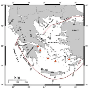
Fig. 3. Scheme of the tectonic setting.

3 Data

In recent years, studies provided evidence that the tectonic framework of Greece and its surroundings resembles to a large extent a converging plate boundary. The principal agents in the geodynamic evolution of the area are the col-lision and subduction in the southern part of the Aegean in a principal SWNE direction, the eastward motion of the Adri-atic microplate in the NW, the westward motion of the Turk-ish microplate, expressed through the activity of the north Anatolian fault in the ENE, and the Kefalonia transform fault, which seems to exercise a major control over the distri-bution of stresses throughout the whole area of Greece and its surroundings (Polimenakos, 1995). These features are shown in Fig. 3.

Burton et al. (2004a,b) carefully created a homogeneous earthquake catalog for Greece (Fig. 4), because of the high seismicity in that region. The catalog contains 5198 earth-quakes during 1900–1999, which are within the area 33◦_– 43◦_{N, 18}◦_–30.99◦_{E, focal depths 1 to 215 km and} magni-tude range 4.0≤Mw≤7.7. These authors used the catalogs and bulletins of the International Seismological Center (ISC), and the researched catalogs of Papazachos and Comninakis (1971), Makropoulos and Burton (1985), Makropoulos et al. (1989), Papazachos et al. (1994) and Papazachos and Papaza-chou (1997). The catalog is complete above magnitude 5.0. All data have been used in the calculations, without removing foreshocks or aftershocks.

Fig. 4. Seismicity in Greece in the the twentieth century.

4 Results and discussion

The results of the optimization for our data set are summa-rized in Tables 1–2. First of all, if we compare these results to the obtained by Jim´enez and Posadas (2006), we can see that the mutual information is always higher with the Ising model. The mutual information increases with decreasing q also. The difference is higher (more information can be ex-tracted) for high magnitude cutoffs in the case of q6=0, and is therefore more interesting for seismic hazard purposes. It is also interesting to note the increase in the “magnetization”, approaching the 50% of active cells (so approaching the null magnetization) with a higher mutual information.

Now, we analyze the behavior of the transition probabili-ties obtained, to find out if they follow an Ising scheme or not. With regard to the energy threshold criterion (q=1), we have the following results. For energy thresholds cor-responding to magnitudes (m) of 4 and 5: An inactive cell with “energy” higher than or equal to 0 (E in Eq. 5) tends to change its state with a probability of 55% in average. When the neighorhood’s state is E<0, and hence the surrounding activity state is the same of the central cell’s activity, its state is reinforced at the next interval of time with high probabil-ity (60–100%). If the cell is active, for E≥0, there are some changes to inactivity, but it mostly tends to the activity. How-ever, with E<0, the trend is to continue the activity.

By using a magnitude threshold of 6, the trend is to in-activity, both for active and inactive cells. However, we can see that the configurations with E<0 for an inactive cell have higher probabilities of going on inactive (80–100%, and not 50–60% as for E≥0), and, for an active cell, for E≤−4 the cell continue clearly active (85% in average). With magni-tude threshold of 7, there is no configurations for inactive cells and E≥0, neither active cells with E≤3, so that these energies are not easily reached by the cells. An inactive cell, with E<0 tends to inactivity with 95–100% probability. An active cell with E>4 tends to change its activity.

Fig. 5. Example of correlation functions for real and simulated pat-terns for q=1, and m=4. The radius (r) refers to the cell’s distances.

In general, an Ising behavior is found, in particular for “en-ergies” lower than 0, when the surrounding activity state is the same of the central cell’s activity, which is a consequence of the clustering found in seismic activity (Aki, 1956; Pe˜na et al., 1993).

We now analyze the correlation functions for the simulated and real patterns (Fig. 5). In the example we can see they are very similar. It is interesting to point out that there is cor-relation up to r=10 (being r the distance in cells) in all the cases with m=4−6, which is nearly the length of the lattices. The number of active cells, or “magnetization”, is close to 50%, so that we have wide domains of active or quiescent cells with correlations comparable to the system length. In percolation theory, this is related to a state near the critical point. In this case, the correlation function is a power law. We found the relationship between the correlation and r fol-lows a straight line in the bi-logarithmic scale, with a corre-lation coefficient of around 0.75 in these cases, up to r=10. However, for m=7 the correlation falls off earlier, around

r=5. This, and the fact that high magnitudes are difficult to

reach, are related to the “magnetization” values found. The transition probabilities for equally energetic states (in the sense of the neighborhood configuration), but different initial state of the central cell, are not the same. In gen-eral, lower “energies” are needed to change the state of an initially active cell, so that the exchange with the external field, B, behaves in an opposite way than the exchange with the neighboring activity. So, B must be lower than 0. In-tuitively, without surrounding exchange, if a cell is inactive a higher external field should increase its probability of be-coming active (E≥0), and an active cell should continue its activity with an increase of the external field. This external field could be a result of either boundary conditions or inter-actions with the ductile part corresponding to each cell.

The fact that for configurations with E<0 (the surround-ing activity state is the same of the central cell’s activity), its state is always reinforced (both active and inactive), is a clear

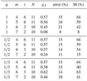
Table 1. Results of the maximization of the Ising model with an energy threshold criterion for Greece (M is the averaged “magneti-zation”, or number of active cells).

q m t N µI error (%) M (%) 1 4 6 11 0.57 15 64 1 5 6 11 0.56 16 59 1 6 3 10 0.45 21 42 1 7 2 10 0.08 8 8 1/2 4 6 11 0.57 15 64 1/2 5 6 11 0.57 15 59 1/2 6 3 10 0.57 14 54 1/2 7 2 10 0.24 11 15 1/3 4 6 11 0.57 15 64 1/3 5 6 11 0.58 15 60 1/3 6 3 10 0.62 14 63 1/3 7 2 10 0.46 18 41

Table 2. Results of the maximization of the Ising model with a num-ber of events criterion (q=0) for Greece (m is the average magni-tude threshold between time intervals and M is the averaged “mag-netization”, or number of active cells). First row: α1criterion;

sec-ond row: α2 criterion; third, by using all the realizations of the

fluctuations up to a determined interval of time also with α2

crite-rion.

m t N µI error (%) M (%)

6.8 3 11 0.50 15 30 6.8 4 10 0.56 18 36 5.9 50 10 0.91 3 45

feature of Ising-like behavior. Taking into account this, an active region loads its neighborhood when it releases energy, a feature contained in the Cellular Automata used to simu-late the seismicity in the literature (Olami et al., 1992; Bar-riere and Turcotte, 1991; Burridge and Knopoff, 1967). That leads to the activation of neighboring areas, if they were close to the rupture point. However, the results obtained here also point out that an active region becomes quiescent because of the neighboring quiescence. This is in accordance with Grif-fith’s principle, in which cells are broken when the release in elastic energy exceeds the surface energy cost (Toussaint and Pride, 2004); if a cell releases energy and the surround-ing areas are not near the rupture point, they will absorb this energy in an elastic way, without becoming active, so that when the initially active cell releases all the exceeding en-ergy, it becomes inactive as well. When E≥0 the transition to changing the state is less clear, mainly because of the non-uniformity in the stress field, that is, B is different for each cell, as exposed before.

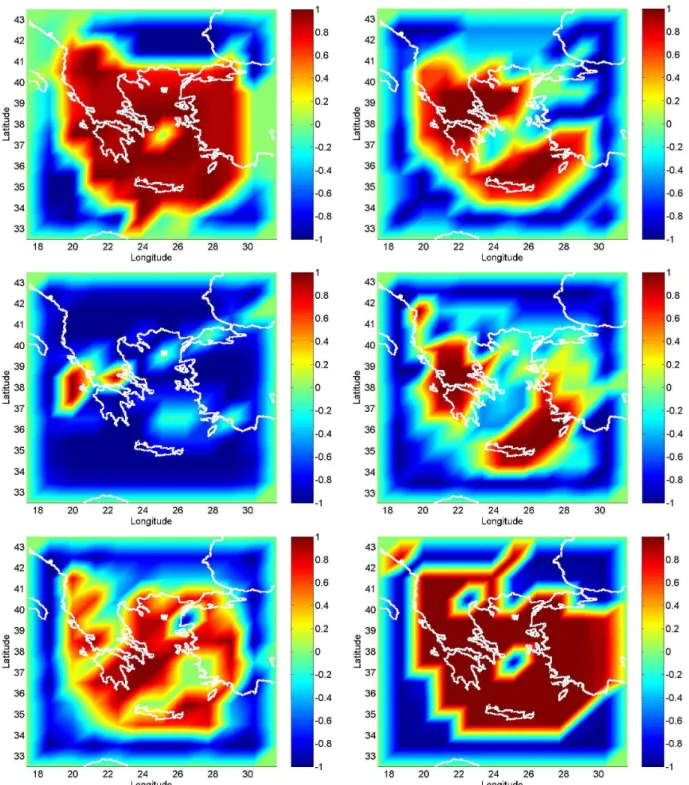
Fig. 6. Probabilistic Activation Maps for the next intervals of time for Greece (a: with q=1/3, the maps for m=4 (16 years), m=5 (16 years), and m=6 (33 years) are very similar, so we show the last one; b: q=1/3, m=7 for 49 years; c: q=1/2, m=7 for 49 years; d: with q=0, first row in Table 2 for 33 years; e: q=0, second row in Table 2 for 25 years; and f: q=0, third row in Table 2 for 2 years).

The results for q=1/2 are as follows. With Benioff strain threshold equivalent to m=4−5, the results are the same as above. For m=6 is also very similar to the former case. How-ever, more configurations are found. Anyways, for E<0 the trend is to continue the previous state, active or inactive. And

for E≥0 there are more probabilities of exchanging the state. For m=7 we found more configurations as well. An inac-tive cell will continue its state, in general, but an acinac-tive cell with E≥0 will change its state. As can be seen, the behav-ior is very similar. It is also very similar for q=1/3, the

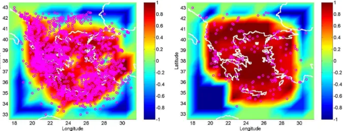
Fig. 7. Probabilistic Activation Maps for the next intervals of time for Greece with q=1/3 using data up to the beginning of the last interval of time found by the method (from left to right, m=5, by using 5 intervals, and m=6 with 2 intervals only). The circles represent the seismic events with magnitude greater than the corresponding threshold found in the data set in the next interval (the sixth for m=5 and the third for

m=6).

difference being in the higher number of active cells with in-creasing magnitude cut off (take into account that a lower q implies a higher weight in smaller earthquakes). The result is an increase in the mutual information between past and fu-ture states, and a proximity to the “null magnetization”. In that case, the system behaves in the closest way to the Ising model, which is a model for phase transitions (long-range correlations, clustering and null magnetization).

For q=0, we have different behaviors, depending on the statistical formulation. If we remove the mean and divide by the standard deviation of the current interval of time (first row in Table 2), the rules are similar to that detailed above. In general, an inactive cell tends to be inactive (80% in av-erage). An active cell tends to be active (90–100%) when

E<0, but there are some configurations for E≥0 when the

probabilities are higher to changing its state. However, if we use the mean and the standard deviation of the whole cata-log (in a mean field approximation), the states tend to be the same, independent of the interaction’s “energy”. No high E is found, neither active or inactive cells. This is more preva-lent when all the realizations are included in the calculations. In this case, the state of the cell is almost completely inde-pendent on the surroundings, and the continuity in the state has 95–100% probability. Although it is more accurate to use the number of the events, we can not recover their ener-getic weight; we only can mark the regions of highest future activity, and estimate the average threshold for the activity between the different intervals of time.

The corresponding Probabilistic Activation Maps for the next intervals of time with q=1/3 and q=0 are shown in Fig. 6. The Probabilistic Activation Maps show the proba-bility of becoming active in the next interval of time for each Stochastic Cellular Automaton calculated. Since the model

takes into account activity (+1) and quiescence (−1), a prob-ability p of becoming active corresponds to 1−p probprob-ability of quiescence, and the scale has been modified from [0,1] to [−1,1] to highlight the Ising behavior. The maps are slightly smoothed in the corners of the cells, because the size of the cells that maximize the mutual information is too big, so that the display is more understandable. We choose q=1/3 for the energy thresholds because it has a higher amount of infor-mation, in particular for higher magnitudes and also because the maps obtained for q=1 are very similar to those found in Jim´enez and Posadas (2006), and the maps with q=1/2 have quite similar features to the shown here, except for m=7.

As in previous works for the Iberian Peninsula (Jim´enez et al., 2005), and for Greece (Jim´enez and Posadas, 2006), the lower number of cells usually maximize the mutual in-formation, by providing the higher dependence between the states, and reflects the large scale of earthquake occurrence. The same discussion as the one in Jim´enez and Posadas (2006) holds for the spatial results found. Wells and Copper-smith (1994) provide widely accepted relationships between magnitude and fault rupture length. Burton (1996) used such relationships to illustrate what might be seen as reasonable spatial constraint on an earthquake prediction, the point be-ing that larger earthquakes are not best thought of as point sources (epicenters) but as fault lengths needing large vol-ume (cell size) to store sufficient strain energy. Activity at high magnitude levels might need the resources of several cells if cells are small. He modeled a region schematically as a grid and, superimposed onto this area were the specimen subsurface rupture lengths. For example, a magnitude 7.5 Ms earthquake might be left floating within an 13 750 km2area unless other constrains are applied. We found that for mag-nitude thresholds of 4 to 5 the optimum cell was of around

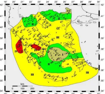
Fig. 8. Map with the seismic hazard zones of Greece (Geophys. Lab. A.U.TH. and ITSAK, 2002). The p.g.a. values for each zone are: I) 0.08–0.13, II) 0.13–0.22, III) 0.22–0.30, IV) 0.30–0.45.

13 300 km2, and 16 000 km2for magnitude 6 and 7. Our re-sults are slightly higher than those proposed by Burton, but in the same order (note that no constrains are imposed to the cells). There is a qualitative change in the patterns for m≥6: the optimum area increases, and the active cells are not so clustered. This roughly corresponds to the threshold of clear spatial resolution, when the subsurface rupture length be-comes about 25 km, and the event cannot be regarded as a point source (Burton, 1996).

A test have been made by using data only from 1901 to 1984, and magnitude threshold of 5 (where the catalog is complete) to calculate the Probabilistic Activation Map. The same test has been made for magnitude threshold of 6, but with data from 1901 to 1967. In Fig. 7 the correspondent maps and the seismicity from the last interval up to 1999 are shown. The events recorded after the data used for the model are found in the higher probability regions in most of the cases. Note that no events after 1984 (m=5) and 1967 (m=6) were used to calculate neither the transition probabil-ities, neither the maps. The only information used was the result found by means of the Kullback-Leibler distance of period of time and cell size needed. A larger catalog has to be used. In both cases, the mutual information found was lower than the obtained by using the whole catalog. It is also remarkable that the transition probabilities follow the same Ising scheme explained before. Unfortunately, we cannot test higher magnitude thresholds because of the time peri-ods needed (50 years), obtained by maximizing the mutual information.

The seismic hazard in Greece was analyzed by Burton et al. (2003) and Burton et al. (2004a,b), who provided maps

for the strong ground acceleration occurrence in that region, as well as maximum magnitudes expected. It has to be noted that our results deal with probabilities of surpassing certain energy releases in the areas by means of a two dimensional spatio-temporal model, and do not include attenuation laws. Taking this into account, our results are very similar to that obtained by these authors. In particular, the maps of max-imum magnitude expected for a period of 50 years in Bur-ton et al. (2004a,b) is nearly the same as ours (in particular,

q=1/3). With regard to the maximum p.g.a. (peak ground

acceleration) expected the major difference is that they de-rive low values for the southeast along the Hellenic Arc in Crete, where, as they point out, although large magnitudes are expected, focal depths are also quite large. Therefore, their maps do not reflect a high value for the p.g.a. How-ever, Papaioannou and Papazachos (2000) give the maximum probabilities for the occurrence of strong-motion (I ≥V I I ) for the period 1996–2010 to these regions. Their map shows the same places as ours for m=6 as most probable of strong motion events, with a time-dependent estimation. As be-fore, they provide intensity values, so that both results are not completely comparable. At this respect, the present re-sults are more accurate to the previous one with no Ising-like model (Jim´enez and Posadas, 2006). For a clearer exposi-tion, in Fig. 8 we show the seismic hazard map provided by Geophys. Lab. A.U.TH. and ITSAK (2002), similar to the described above.

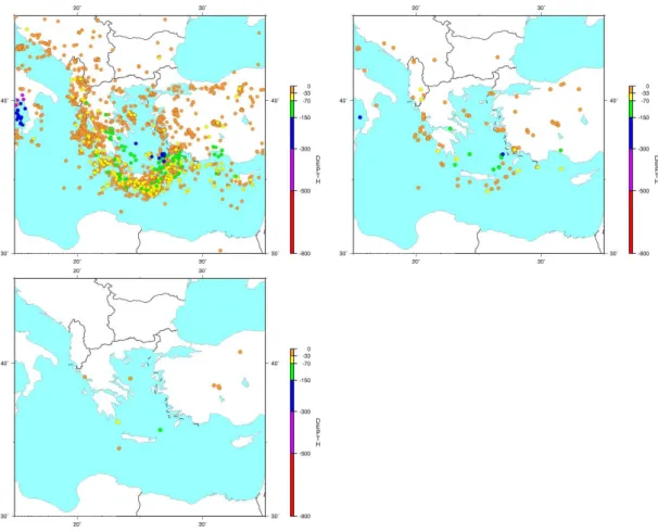
The real seismicity after the data set used is shown in Fig. 9 (NEIC, National Earthquake Information Center). The Prob-abilistic Activation Maps for energies corresponding to m=4 and m=5 are close to the real seismicity after the data in that area, and they correspond to a background seismicity in the whole area. With regard to the other maps the narrow span of time (only 7 years after the data), we cannot extract any definite conclusion. It will be interesting to see how the seis-micity behaves the next years to answer this question. The main difference between this model and that used in Jim´enez and Posadas (2006) in the forecast corresponds to the mag-nitude threshold of 7. No earthquake is supposed to occur in the next 50 years following Jim´enez and Posadas (2006) but, as can be seen in this work, the Southern Aegean Sea, Dodecanese Islands and Crete, in one hand, and Ionian Is-lands, central Greece and North Anatolian Fault, in the other. In fact, the higher probabilities for earthquakes of magnitude equal to or greater than 7 are found in the principal faults of the region, as explained in Sect. 3. So the places where these extreme events are foreseen are coherent with the tectonical setting.

The important point of this method is the proposal of a par-ticular time (50 years since the last data used) to be checked. The time-dependence it’s important to obtain the transition probabilities. If we average the energy, we should know the temporal and spatial scales for the averaging. If we use the same as the found by the model, the patterns change, so it would not be time-independent. In a time-independent

Fig. 9. Actual seismicity after 2000 (from left to right, and top to bottom, m=4, m=5, and m=6. No m>7 earthquakes have occurred).

estimation, the energy (or magnitude) used for the calcula-tions is usually the highest found in each seismogenetic zone, that may change in time, depending on the time span of the catalog. So, if we compare the patterns with the highest mag-nitudes, or add up the energy, it is time-dependent. For ex-ample, in the catalog, there are some earthquake whose mag-nitude are grater than 7 in the Anatolian region, and it would be included in a time-independent estimation. However, the Probabilistic Activation Maps found do not mark this place as likable to surpass this magnitude. Note that since the time span is long and the spatial resolution is low, it can’t be viewed as a prediction, but as a large-scale forecasting, or, as we propose, a Probabilistic Activation Map, but not in a static sense. It is also to be noted that there are no attenua-tion laws, no site responses applied, so the meaning of these Probabilistic Activation Map are the probabilities of surpass-ing certain energies (magnitudes) in the different places of the studied area.

5 Conclusions

The Ising model tested, although it is a very simplified one for describing the seismicity, points out some interesting

be-haviors: first, the Benioff strain contains more information about the sequence of patterns, and it is more predictable, than direct energy measures. In the same way, criterion based upon the size of the events (q=1/3) contains more informa-tion between consecutive patterns than the previous criteria, in agreement with the Hurst’s exponent; second, that the cells tend to adopt the surrounding activation or quiescence (in the sense explained above) as Ising models do; third, that the cells are disposed in wide domains, while the percentage of active and quiescent cells is nearly 50% up to m=6 (which will indicate a “null magnetization”), that could indicate a critical state. But the patterns are the result of the accumu-lation of the energy over intervals of time that span from 15 to 50 years, so we can not conclude that it remains always in a critical state; it means that the higher information is found when this state is reached, and correlations are higher.

The Probabilistic Activation Maps provided are coherent with the previous works made for that area, and with its tec-tonic setting. It also provides different timing for different energy releases, and it can be viewed as a more dynamical seismic hazard information.

The advantages of using this instead of the proposed in Jim´enez and Posadas (2006) are the following: the informa-tion content is higher, in particular for higher energies, so we

“know” better the transitions from one pattern to another; the intervals of time found are lower (for example, for m=5 we go from a 25-year to a 15-year map in the present model), which is more interesting for seismic hazard purposes, and can be better tested; finally, the model (Ising) is related to a broad kind of systems in physics, in particular, statistical mechanic, so that we can use its tools to analyze it.

In conclusion, the Ising-like CA proposed for Greece and surrounding areas reproduces the principal features of the seismicity in the zone, delineates the strong correlation be-tween large areas in the crust, and provides reliable Proba-bilistic Activation Maps, in the sense explained.

Acknowledgements. This work was partially supported by the

MCYT project CGL2005-05500-C02-02/BTE, the MCYT project CGL2005-04541-C03-03/BTE, and the Research Group “Geof´ısica Aplicada” RNM194 (Universidad de Almer´ıa, Espa˜na) belonging to the Junta de Andaluc´ıa. The work of KFT was funded by an NSERC Discovery Grant. The work of AJ was funded by a “Fundaci´on Ram´on Areces” Grant.

Edited by: G. Zoeller Reviewed by: one referee

References

Aki, K.: Correlogram analyses of seismograms by means of a sim-ple automatic computer, J. Phys. Earth, 4, 71–79, 1956. All`egre, C. J. and Le Mouel, J. L.: Introduction of Scaling

Tech-nique in Brittle Failure of Rocks, Phys. Earth Planet Inter., 87, 85–93, 1994.

All`egre, C. J., Le Mouel, J. L., and Provost, A.: Scaling Rules in Rock Fracture and Possible Implications for Earthquake Predic-tions, Nature, 297, 47–49, 1982.

Anghel, M., Klein, W., Rundle, J. B., and Martins, J. S. S.: Scal-ing in a cellular automaton model of earthquake faults, ArXiv Condensed Matter e-prints, 2000.

Bak, P. and Tang, C.: Earthquakes as a Self-Organized Critical Phe-nomenon, J. Goephys. Res., 94, 15 635–15 637, 1989.

Bak, P., Tang, C., and Wiesenfeld, K.: Are Earthquakes, Frac-tals, and 1/f Noise Self-Organized Critical Phenomena, Cooper-ative Dynamics in Complex Systems, edited by: Takayama, H., Springer-Verlag, Tokyo, 1988.

Barriere, B. and Turcotte, D. L.: A scale-invariant cellular automa-ton model for distributed seismicity, Geophys. Res. Lett., 18, 2011–2014, 1991.

Boettcher, S. and Hartmann, A. K.: Reduction of Two-Dimensional Dilute Ising Spin Glasses, Phys. Rev. B, 72, 014 429, http://arxiv. org/abs/cond-mat/0503486, 2005.

Bowman, D. D. and King, G. C. P.: Accelerating seismicity and stress accumulation before large earthquakes, Geophys. Res. Lett., 28, 4039–4042, 2001.

Bufe, C. G. and Varnes, D. J.: Predictive Modeling of the Seismic Cycle of the Greater San Francisco Bay Regiony, J. Geophys. Res., 98, 9871–9883, 1993.

Burridge, R. and Knopoff, L.: Model and theoretical seismicity, Bull. Seism. Soc. Am., 57, 341–371, 1967.

Burton, P. W.: Dicing with earthquakes, Geophys. Res. Lett., 23, 1379–1382, 1996.

Burton, P. W., Xu, Y., Tselentis, G., Sokos, E., and Aspinall, W.: Strong ground acceleration seismic hazard in Greece and neigh-boring regions, Soil Dyn. Earthqu. Eng., 23, 159–181, 2003. Burton, P. W., Xu, Y., Qin, C., Tselentis, G., and Sokos, E.: A

catalogue of seismicity in Greece and the adjacent areas for the twentieth century, Tectonophysics, 390, 117–127, 2004a. Burton, P. W., Qin, C., Tselentis, G., and Sokos, E.: Extreme

earth-quake and earthearth-quake perceptibility study in Greece and its sur-rounding area, Nat. Hazards, 32, 277–312, 2004b.

Carlson, J. M. and Langer, J. S.: A mechanical model of an earth-quake fault, Phys. Rev. A, 40, 6470–6484, 1989a.

Carlson, J. M. and Langer, J. S.: Properties of earthquake generated by fault dynamics, Phys. Rev. Lett., 62, 2632–2635, 1989b. Carpinteri, A. and Pugno, N.: Are scaling laws on strength of solids

related to mechanics or to geometry?, Nature Materials, 4, 421– 423, 2005.

Christensen, K. and Olami, Z.: Variation of the Gutemberg-Richter b values and nontrivial temporal correlations in a spring-block model of earthquakes, J. Geophys. Res., 97, 8729–8735, 1992. Colella, V. S., Klopfer, E., and Resnick, M.: Adventures in

Mod-eling: Exploring Complex Dynamic Systems with Starlogo, Teachers College Press, 2001.

Cover, T. and Thomas, J.: Elements of information theory, Wiley and Sons, 1991.

Daley, D. J. and Vere-Jones, D.: Scoring probability forecasts for point processes: the entropy score and information gain, J. Appl. Probab., 41A, 297–312, 2004.

Geophys. Lab. A.U.TH. and ITSAK: Collection and Procession of Seismological data and computation of seismic hazard map of Greece according to the current Greek Seismic Code and Eu-rocode, Tech. rep., Geophysical Laboratory of Aristotle Univer-sity of Thessaloniki and Institute of Engineering Seismology and Earthquake Engineering (ITSAK), 2002.

Gould, H. and Tobochnik, J.: Thermal and Statistical Physics, avail-able at http://stp.clarku.edu/notes/, 2004.

Gutenberg, B. and Richter, C.: Earthquake magnitude, intensity, energy, and acceleration, Bull. Seism. Soc. Am., 46, 105–145, 1956.

Hirata, T.: A correlation between the b value and the fractal dimen-sion of earthquakes, J. Geophys. Res., 94, 7507–7514, 1989. Hirata, T. and Imoto, M.: Multifractal analysis of spatial

distribu-tion of microearthquakes in the Kanto region, Geophys. J. Int., 107, 155–162, 1991.

Hirata, T. and Imoto, M.: A probabilistic cellular automaton ap-proach for a spatiotemporal seismic activity pattern, Zisin, 2(49), 441–449, 1997.

Jim´enez, A. and Posadas, A. M.: A Moore’s cellular automaton model to get probabilistic seismic hazard maps for different mag-nitude releases: A case study for Greece, Tectonophysics, 423, 35–42, 2006.

Jim´enez, A., Posadas, A. M., and Marfil, J. M.: A Probabilistic Seis-mic Hazard Model based on Cellular Automata and Information Theory, Nonlin. Processes Geophys., 12, 381–396, 2005, http://www.nonlin-processes-geophys.net/12/381/2005/. Jim´enez, A., Tiampo, K. F., Levin, S., and Posadas, A. M.: Testing

the persistence in earthquake catalogs: The Iberian Peninsula, Europhys. Lett., 73 (2), 171–177, 2006.

Klein, W., Rundle, J. B., and Ferguson, C. D.: Scaling and Nu-cleation in Models of Earthquake Faults, Phys. Rev. Lett., 78, 3793–3796, 1997.

Klein, W., Gould, H., Tobochnik, J., Alexander, F. J., Anghel, M., and Johnson, G.: Clusters and Fluctuations at Mean-Field Criti-cal Points and Spinodals, Phys. Rev. Lett., 85, 1270–1273, 2000. Kroll, D. M. and Gompper, G.: Wetting in fcc Ising

antiferromag-nets and binary alloys, Phys. Rev. B, 36, 7078–7090, 1987. Mai, P. M. and Beroza, G. C.: Source Scaling Properties from

Finite-Fault-Rupture Models, Bull. Seism. Soc. Am., 90, 604– 615, 2000.

Makropoulos, K. C. and Burton, P. W.: A catalogue of seismicity in Greece and adjacent areas, Geophys. J. R. Astron. Soc., 65, 741–762, 1985.

Makropoulos, K. C., Drakopoulos, J. K., and Latousakis, J. B.: A revised and extended earthquake catalogue for Greece since 1900, Geophys. J. Int. Res. Note, 98, 391–394, 1989.

Nakanishi, H.: Cellular-automaton model of earthquakes with de-terministic dynamics, Phys. Rev. A, 41, 7068–7089, 1990. Nakanishi, H.: Statistical properties of the cellular-automaton

model for earthquakes, Phys. Rev. A, 43, 6613–6621, 1991. Olami, Z., Feder, H. J. S., and Christensen, K.: Self-organized

criti-cality in a continuous, nonconservative cellular automaton mod-eling earthquakes, Phys. Rev. Lett., 68, 1244–1247, 1992. Omori, F.: On the aftershocks of earthquakes, J. Coll. Sci., 7, 111–

200, 1895.

Otsuka, M.: A simulation of earthquake occurrence, Phys. Earth Planet. Inter., 6, 311–315, 1972.

Papaioannou, C. A. and Papazachos, B. C.: Time-independent and time-dependent seismic hazard in Greece based on seismogenic sources, Bull. Seismol. Soc. Am., 90, 22–33, 2000.

Papazachos, B. C. and Comninakis, P. E.: Geophysical and tectonic features of the Aegean arc, J. Geophys. Res., 76, 8517–8533, 1971.

Papazachos, B. C. and Papazachou, C.: The Earthquakes of Greece, Editions Ziti, Thessaloniki, 1997.

Papazachos, B. C., Karakaisis, G. F., and Hatzidimitriou, P. M.: Fur-ther information on the transform fault of the Ionian sea, XXIV Gen. Ass., Europ. Seism. Com., Athens, 19–24 September, 1, 377–384, 1994.

Pe˜na, J., Vidal, F., Posadas, A. M., Morales, J., Alguacil, G., De Miguel, F., Ib´a˜nez, J., Romacho, M., and L´opez-Linares, A.: Space clustering properties of the Betic-Alboran earthquakes in the period 1962–1989, Tectonophysics, 221, 125–134, 1993. Polimenakos, L. C.: Shallow seismicity in the area of Greece: its

character as seen by means of a stochastic model, Nonlin. Pro-cesses Geophys., 2, 136–146, 1995,

http://www.nonlin-processes-geophys.net/2/136/1995/.

Posadas, A. M., Hirata, T., Vidal, F., and Correig, A.: Spatiotem-poral seismicity patterns using mutual information application to southern Iberian peninsula (Spain) earthquakes, Phys. Earth Planet. Inter., 122, 269–276, 2000.

Rundle, J. B.: A physical model for earthquakes, 2. Application to Southern California, J. Geophys. Res., 93, 6255–6274, 1988. Rundle, J. B.: Magnitude-frequency relations for earthquakes using

a statistical mechanical approach, J. Geophys. Res., 98, 21 943– 21 949, 1993.

Rundle, J. B., Turcotte, D. L., Shcherbakov, R., Klein, W., and Sam-mis, C.: Statistical physics approach to understanding the multi-scale dynamics of earthquake fault systems, Rev. Geophys., 41, 1019–1049, 2003.

Rundle, P. B., Rundle, J. B., Klein, W., Martins, J. S. S., Tiampo, K. F., Donnellan, A., and Kellogg, L. H.: GEM plate boundary simulations for the plate boundary observatory: Understanding the physics of earthquakes on complex fault systems, Pure. Appl. Geophys., 159, 2357–2381, 2002.

Ryan, M. J. and Frater, M. R.: Communications and information systems, Argos Press, 2002.

Sammis, C. G. and Smith, S. W.: Seismic Cycles and the Evolu-tion of Stress CorrelaEvolu-tion in Cellular Automaton Models of Finite Fault Networks, Pure Appl. Geophys., 155, 307–334, 1999. Schaap, H. G.: Ising models and neural networks, Ph.D. thesis,

Uni-versity of Groningen, 2005.

Smalley, R. F., Chatelain, J. L., Turcotte, D. L., and Prevot, R.: A fractal approach to the clustering of earthquakes: applications to the seismicity of the New Hebrides, Bull. Seism. Soc. Amer., 77, 1368–1381, 1987.

Sornette, A. and Sornette, D.: Self-organized criticality and earth-quakes, Europhys. Lett., 9, 197–202, 1989.

Sornette, D. and Sammis, C. G.: Complex Critical Exponent from Renormalization Group Theory of Earthquakes: Implications for Earthquake Predictions, J. Phys. I France, 5, 607–619, 1995. Tiampo, K. F., Rundle, J. B., McGinnis, S., Gross, S. J., and Klein,

W.: Mean-field threshold systems and phase dynamics: an appli-cation to earthquake fault systems, Europhys. Lett., 60, 481–488, 2002a.

Tiampo, K. F., Rundle, J. B., McGinnis, S. A., and Klein, W.: Pat-tern Dynamics and Forecast Methods in Seismically Active Re-gions, Pure Appl. Geophys., 159, 2429–2467, 2002b.

Toussaint, R. and Pride, S. R.: Interacting damage models mapped onto Ising and percolation models, ArXiv Condensed Matter e-prints, 2004.

Vicsek, T.: Fractal growth phenomena, World Scientific, 1992. Wells, D. L. and Coppersmith, K. J.: New empirical relationships

among magnitude, rupture length, rupture width, rupture area, and surface displacement, Bull. Seism. Soc. Am., 84, 974–1002, 1994.

Wong, S. K.: A cursory study of the thermodynamic and mechan-ical properties of Monte-Carlo simulations of the Ising model, Ph.D. thesis, University of Notre Dame, Indiana, 2005.