Modeling the effects of water content on TiO2 nanoparticles transport in porous media

HAL Id: hal-03049671

https://hal.archives-ouvertes.fr/hal-03049671

HAL is a multi-disciplinary open access archive for the deposit and dissemination of sci-entific research documents, whether they are pub-lished or not. The documents may come from teaching and research institutions in France or abroad, or from public or private research centers.

L’archive ouverte pluridisciplinaire HAL, est destinée au dépôt et à la diffusion de documents scientifiques de niveau recherche, publiés ou non, émanant des établissements d’enseignement et de recherche français ou étrangers, des laboratoires publics ou privés.

Modeling the effects of water content on TiO2

nanoparticles transport in porous media

Ivan Toloni, Francois Lehmann, Philippe Ackerer

To cite this version:

Ivan Toloni, Francois Lehmann, Philippe Ackerer. Modeling the effects of water content on TiO2 nanoparticles transport in porous media. Journal of Contaminant Hydrology, Elsevier, 2016, 191, pp.76-87. �10.1016/j.jconhyd.2016.05.006�. �hal-03049671�

Modeling the Effects of Water Content on TiO2 Nanoparticles Transport in

Porous Media.

Ivan Toloni*, François Lehmann, Philippe Ackerer LHyGeS, Université de Strasbourg/EOST – CNRS

1 rue Blessig, 67084 STRASBOURG Cedex FRANCE

Submitted to Journal of Contaminant Hydrology

First submission: March 21, 2016.

Second submission: May 17, 2016.

Abstract

The transport of manufactured titanium dioxide (TiO2, rutile) nanoparticles (NP) in porous media

was investigated by metric scale column experiments under different water saturation and ionic strength (IS) conditions.

The NP breakthrough curves showed that TiO2 NP retention on the interface between air and

water (AWI) and the interface between the solid and the fluid (SWI) is insignificant for an IS equal to or smaller than 3 mM KCl. For larger IS, the retention is depending on the water content and the fluid velocity. The experiments, conducted with an IS of 5 mM KCl, showed a significantly higher retention of NP than that observed under saturated conditions and very similar experimental conditions.

Water flow was simulated using the standard Richards equation. The hydrodynamic model parameters for unsaturated flow were estimated through independent drainage experiments. A new mathematical model was developed to describe TiO2 NP transport and retention on SWI and AWI. The model accounts for the variation of water content and water velocity as a function of depth and takes into account the presence of the AWI and its role as a NP collector. Comparisons with experimental data showed that the suggested modeled processes can be used to quantify the NPs retentions at the AWI and SWI. The suggested model can be used for both saturated and unsaturated conditions and for a rather large range of velocities.

Keywords: titanium dioxide; column experiments; retention model; unsaturated porous medium;

1. Introduction

Currently, manufactured nanoparticles (NPs) are present in a variety of materials and products according to their properties. TiO2 NPs that are present, for example, in clothing, sunscreens and

paintings, are the second most produced NPs worldwide (Adam et al., 2015). As for other NPs, their potential impact on the environment is still quite unknown. Therefore, to assess the NP life cycle, it is important to study NP mobility through ecosystems.

Although numerous research studies were conducted on the retention of TiO2 NP in saturated

porous media (e.g., Solovitch et al., 2010, Liang et al., 2013b, Toloni et al., 2014), only a few studies have been published on the retention of TiO2 NP in unsaturated porous media (Chen et

al., 2008, Chen et al., 2010, Fang et al., 2013). Transport experiments under unsaturated conditions present greater experimental difficulties, particularly related to the control of the water content profile. The role of the interface between air and water (AWI) in NP retention is not yet completely understood. According to Fang et al. (2013), the presence of the AWI does not enhance the retention of TiO2 NP, whereas it increases the retention of TiO2 NP for Chen et

al. (2008). Therefore, a doubt still persists on whether the saturation level affects the NP retention. According to studies on the transport of other types of NP and colloids, the saturation level affects the NP retention and the AWI can be a collector for charged particles, depending on the chemical parameters (Corapcioglu and Choi, 1996, De Novio et al., 2004, Bradford and Torkzaban, 2008, Kumahor et al., 2015, Knappenberger et al., 2015).

To the authors’ knowledge, TiO2 NP retention in unsaturated porous media has never been

attachment-detachment model, eventually adding a retardation term (Liang et al., 2013b; Kumahor et al., 2015). Contrary to colloids (Lenhart and Saiers, 2002, Anders and Chrysikopoulos, 2009, Zhang et al., 2012, Syngouna and Chrysikopoulos, 2015), the saturation level and the presence of the interface between air and water has never directly been taken into account for NP transport modeling in unsaturated porous media. The studies on colloid transport assume the retention as proportional to the AWI surface, which is very difficult to measure and generally is estimated from the volumetric air volume of the porous medium.

The objective of this study is to better understand the role of the water content and AWI on NP retention and to propose a new model that is able to address saturated and unsaturated conditions. Sand column experiments were conducted with TiO2 NPs with different chemical compositions

of the injected fluid and under varying water content profiles. The hydrodynamical conditions were simulated by Richards’ equation to estimate the water velocity and water content inside the column. The transport model, which takes into account the presence of the AWI and its role as a NP collector, was developed based on previous results obtained by Toloni et al. (2014) under saturated conditions.

2. Experimental Methods 2.1 TiO2 Nanoparticles

A 50 mg L-1 aqueous suspension of TiO2 NPs was prepared by diluting a commercial rutile

dispersion (NanoAmor 7012WJWR, 15 wt%, 5-30 nm) with deionized (DI) water and setting the ionic strength (IS) and pH values with KCl and KOH. The TiO2 NP suspension had an isoelectric

point at a pH of approximately 6 and a Z-average NP size between 70 and 100 nm. Since a pH of 10 resulted in a stable NP dispersion and minimized NP interactions with the sand surface, this

pH was chosen to minimize NP deposition. More details are provided in Toloni et al. (2014) and Toloni (2015), which used the same NP suspension.

2.2 Sand

The porous medium was composed of 96.7% quartz sand (K30, Kaltenhouse, France), with an average size of d50 = 490 m, a coefficient of uniformity of Cu = 1.6, a bulk density of b=1.75

g/cm3 and trace amounts of orthoclase and variscite. The medium was cleaned before packing through acidic and basic washings to remove metal oxides, impurities and colloidal particles, as described in Toloni et al. (2014).

2.3 Column Experiments

Two different setups were used to perform the experiments, as in Toloni (2015). The drainage setup (column of length 28cm and of diameter 28cm with in situ sensors) was used to estimate hydrodynamic parameters, while the NP transport experiments were performed on a similar type of column of smaller dimension (length 15.2 cm, diameter 3.75cm). To avoid perturbations due to the interactions between the NPs and the metal components of the TDR probes, the experimental setup for the NPs transport experiments did not include in situ sensors.

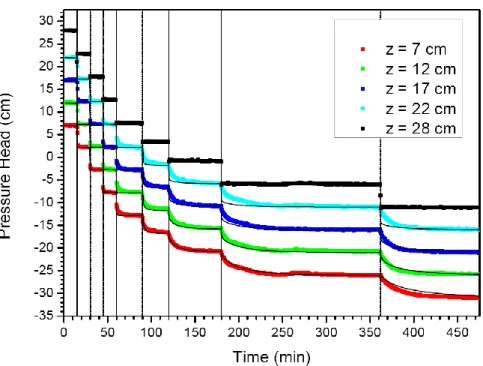
A Plexiglas column was employed for the drainage experiments. The bottom of the column was linked by a plastic tube to a vertically mobile water reservoir, allowing for control and prescribing the water pressure head at the column bottom. Sensors were placed inside the column to monitor the water content, pressure head and temperature. The necessity of accommodating the sensors justifies the relatively large column diameter. The water content was measured by TDR probes (ML2x, Delta-T Devices Ltd, Cambridge, UK). Two probes were installed 7 cm and 17 cm below the sand surface. The pressure head was measured by five tensiometers (35 X,

Keller AG, Winterthur, Switzerland), installed 7 cm, 12 cm, 17 cm, 22 cm, and 28 cm below the sand surface. The column was wet-packed as uniformly as possible with cleaned sand. Careful and uniform sand packing is important for the water content sensors and tensiometers to work properly because a good contact with sand grains is required. In the packed sand column, the water level is controlled by the position of the water reservoir. During column filling, the reservoir connected to the column bottom is located at the level of the sand surface to ensure saturation. Once the column is filled, the reservoir is lowered, inducing drainage and decreasing water content. The reservoir was moved down step by step from 28 cm over the column bottom to 10 cm below the column bottom, corresponding to a prescribed pressure of -10 cm (Figure 1). The reservoir was moved after the hydrodynamical equilibrium was reached, i.e., no flow at the column bottom. The lower the reservoir position was, the more time was required to achieve stable values for the water content and pressure head: a complete step by step drainage required 6 hours.

A Plexiglas flow cell from Soil Measurement Systems, Tucson USA was adopted for the NP transport experiments. The flow cell consisted of a tube that holds the porous medium and two removable end-plate assemblies, one mounted on each end of the tube. The flow cell was equipped with two types of end-plates: regular end-plates and perforated end-plates, which were intended to expose the sand surface to the atmospheric pressure. Ultraviolet absorption values were measured automatically every 5 s throughout the experiments for both the inlet and outlet flows by means of on-line sensors. The transport experiments consisted of injections of the TiO2 NP solution at the top of a column under unsaturated steady state flow conditions and under four

IS treatments (0-2-3-5 mM KCl). Each experiment was performed according to the following protocol:

1. The column was carefully wet-packed with cleaned sand, obtaining a saturated porous medium. A 2-cm layer of glass beads held the porous media in place at the bottom of the column. This arrangement was necessary because it was not possible to find a filter or a membrane that did not retain the TiO2 NP. It has been previously verified that glass beads

do not retain NP under the adopted experimental conditions.

2. The porous medium was equilibrated at the desired IS and pH, with 20 pore volumes (PV) of electrolyte solution (Toloni, 2015).

3. A water flow of 0.0012 cm s-1 was then applied at the top of the column through a peristaltic pump, and the sand surface was exposed to atmospheric pressure. The pump’s tubes were replaced before each experiment to ensure stable flow rates. A prescribed pressure head of -14 cm at the column bottom was applied to enhance column drainage. A vacuum chamber was not used because its use would imply the use of a membrane. This operation brings the column from an initial hydrostatic profile to a new unsaturated profile. The cumulative water mass of the drainage was measured online.

4. Once a steady state flow condition was reached (i.e., the flow rate at the outflow becomes equal to the injected water flow rate), 2.5 PV of the 50 mg/L TiO2 NP suspension were

injected in the column. The NP concentration was monitored by flow through cells. 5. To obtain a complete breakthrough curve (BTC), the electrolyte solution was injected for

approximately two more PV.

3. Modelling of flow and NP transport 3.1 The water flow model

The movement of water in an unsaturated porous medium is described by the general equation of flow (Pinder and Celia, 2006):

s Sat r Sat r D h h S K K (h) 1 t t x x h K K (h) 1 x q    __   _         _{ } _   _  _     (1)

where Ss [L-1] is the specific storage, h [L] is the pressure head, t [T] is the time,  [-] is the volumetric water content, x [L] is the depth, Ksat [LT-1] is the saturated hydraulic conductivity, Kr is the relative hydraulic conductivity and q_D [LT-1] is the Darcy velocity. Here, the equation is

presented in its one-dimensional form. The solid matrix is assumed to be incompressible, and the air phase is assumed to be highly mobile and instantaneously in equilibrium with the atmosphere.

The relations Kr(h) and h) are required to solve the general equation of flow. The Mualem-van Genuchten Model is adopted:

 

 

where r [-] is the residual volumetric water content, s [-] is the saturated volumetric water

content, n [-] is the pore size distribution index,  [L-1] is related to the inverse of the characteristic pore radius, l [-] is the pore connectivity parameter and Se [-] is the effective saturation.

An estimation of the Mualem-van Genuchten hydrodynamic parameters is necessary to solve the general equation of flow and model the water content and velocity distributions over the columns. The relationship between the pressure head (h) and water content (), expressed by the hydrodynamic parameters, was investigated by independent drainage experiments. The Mualem-van Genuchten model parameters (, r, s, n, l, Ksat) were estimated from the water content data

and pressure head data of the step by step drainage experiment. The inverse problem was solved through the Levenberg-Marquardt optimization algorithm. The inverse problem was solved through the Levenberg-Marquardt optimization algorithm. The gradient of the objective function with respect to each parameter was calculated analytically as in Hayek et al. (2008) and Beydoun et al. (2006). In Figure 1, the solution for the pressure head data is shown. A zero flow boundary condition was applied at the top of the column, while the pressure head measured at the tensiometer installed 28 cm below the sand surface was taken as the lower boundary conditions. The hydrostatic profile was taken as an initial condition. To reduce the dimensionality of the problem and considering that the van Genuchten parameters are often correlated, the value of the pore connectivity parameter l was set to 0.5 and the residual water content r was set to zero. The

chosen l value is often adopted in the literature (Abbaspour et al., 2001; Wollschlaeger et al., 2009). The residual water content is a parameter that is very difficult to measure directly because measurements at very low saturation values are time consuming to ensure equilibrium. In the literature, values between zero and 0.05 can be found. For simplicity and because the NP

transport experiments were performed under similar wet conditions, r was fixed to zero. In the

evaluation, different sets of initial parameter values were tested to identify potential local minima. The solution of the inverse problem was the same for all of the initial parameters sets. The parameters were weakly correlated. The optimized values for s, , n and Ksat were 0.38 ±

0.0003, 0.037 ± 0.00006 cm-1, 12.24 ± 0.05 and 0.23 ± 0.0003 cm/s, respectively. Moreover, the longitudinal dispersivity (L = 0.20 ± 0.01 cm) was estimated through tracer experiments

conducted with 3 pore volumes (PV) of KCl.

3.2 Modeling of TiO2 Nanoparticle Transport in unsaturated conditions

The transport and retention of TiO2 NP through the unsaturated porous media was initially

simulated using the convection-dispersion equation model coupled with a kinetic retention term:

D q c θc s c ρ θD t t x x x   _  _    _          (4) a s θk Ψc t     (5) max s Ψ 1 s   (6)

where  [-] is the volumetric water content, c [M L-3] is the NP aqueous phase concentration,  [M L-3] is the bulk density of the porous media, s [M M-1] is the NP solid phase concentration, t is the time [T], x [L] is the distance from the column inlet, D [L2 T-1] is the hydrodynamic dispersion coefficient, qD [L T-1] is the Darcy velocity, ka [T-1] is the attachment coefficient,  [-] is a retention function and smax [M M-1] is the maximal solid phase concentration. Adopting this model, NPs were supposed to interact with a limited amount of attachment sites (smax) in porous

(Bradford, 2006). Therefore, as the number of occupied sites increases throughout the experiment, the probability of an NP encountering a free site decreases (Ryan and Elimelech, 1996). The NP BTCs were modeled with Equations 4, 5 and 6, optimizing smax and ka. This model, referred to as model 1S, is quite standard and assumes that the retention parameters are constant along the column profile.

Because the fluid velocity and the water content change over the column’s length under our unsaturated experimental conditions, different retention models were developed to take into account the influence of the water velocity and of the water content. Unlike in the 1S model, in these models, smax and ka are not constant, but vary along the column profile. Through the water content profile, these models can potentially account for NP retention at the AWI or at the interface between the sand and water (SWI).

Under saturated flow conditions, Toloni et al. (2014) found that the fluid velocity affects the NP retention and suggested the following expressions for smax and ka:

max 1 0 s  a (7) D a pc 0 50 q 3(1 ) k 2d       (8)

where a1 [MM-1] and pc[-] are empirical parameters,  is the porosity [-], d50 is the average

grain size [L], 0 [-] is the single collector efficiency described by the classic filtration theory

(Tufenkij and Elimelech, 2004), pcis a function of the grain geometry, (1 ) represents the

volume of the solid phase, and

q /



The NP BTCs were modeled modifying Equations 7 and 8, assuming that retention only occurs at the SWI. The obtained model explicitly takes into account the potential retention at the SWI along the profile as a function of the water velocity and water content (1S_SWI model):

SWI D q c θc s c ρ θD t t x x x   _  _    _          (9) SWI a SWI SWI SWI max s _{θ c 1} s t k s      _  _  _{ } (10) 2/3 SWI SWI max 1 0 s s a         (11) SWI s D SWI a 0 pc 50 3(1 ) q k 2d       (12)

where sswi [M M-1] is the NP concentration at the SW, and a1swi [M M-1] and pcswi [-] are

empirical parameters that must be calibrated. Equations 7 and 8 were modified to take into account the assumed reduced accessibility of the sand surface under unsaturated conditions, even if the fluid phase was assumed to be continuous over the column to ensure pressure transmission. In Equation 8, the porosity  was replaced by the saturated water content s in the numerator

(Bradford et al., 2008). The variation of accessibility of the sand surface was assumed to be proportional to the variation of the specific surface s [L2M-1]. Assuming that the grain geometry

of our porous medium can be approximated by spheres and that the effects of water content variations on the specific surface are equivalent to the effects of porosity variations, we used the model suggested by Emmanuel and Berkowitz (2005):

2/3 0 0 s   s       (13)

where

s

Equations 11 and 12 can be used for both saturated and unsaturated porous media: In the case of water saturation, they become equations 7 and 8.

The NP BTCs were also modeled assuming that if the porous medium is unsaturated, the retention at the SWI can be neglected and NPs are retained exclusively at the AWI (1S_AWI model): AWI D a q c θc s c θD t t x x x   _{ }  _    _          (14) AWI AWI AWI a AWI max a s _{θ c 1} s t k s      _  _  _{ } (15) 3

AWI AWI AWI

max 1 0

s s a  _1  _



  (16)

AWI s D AWI AWI

a 0 pc 50 s 3( ) q k 1 2d          _  _  _  _ (17)

In the above equations, sawi [M L-3] is the NP concentration at the AWI,    _a





calibrated. The single collector efficiency 0awi was modified to account for the unsaturated

conditions:  is -dependent and not -dependent (Tufenkij and Elimelech, 2004). We assumed that the retention at the AWI depend on a (Chen et al., 2008). Following Zhang et al. (2012),

smax for the retention at the AWI was written as proportional to





1  / . Equations 16 and 17 become zero for a saturated porous medium.

To consider retention at both the AWI and SWI, a two-site retention model was also applied (2S model):

SWI AWI D a q c θc s s c ρ θD t t t x x x   _  _{ }  _    _           (18) SWI SWI SWI a SWI max s _{θ 1} s c k t s      _  _  _{ } (19) AWI AWI AWI a a AWI max s s c θ θk 1 t s    _{ }    _{ } (20)

where the first site (Equation 19) describes the NP retention at the sand grain surface and the second site (Equation 20) describes the NP retention at the interface between water and air. The 2S model has the parameters of both the 1S_SWI and 1S_AWI models; therefore, four parameters must be calibrated.

4. Results and Discussion

4.1 Water Content Profiles

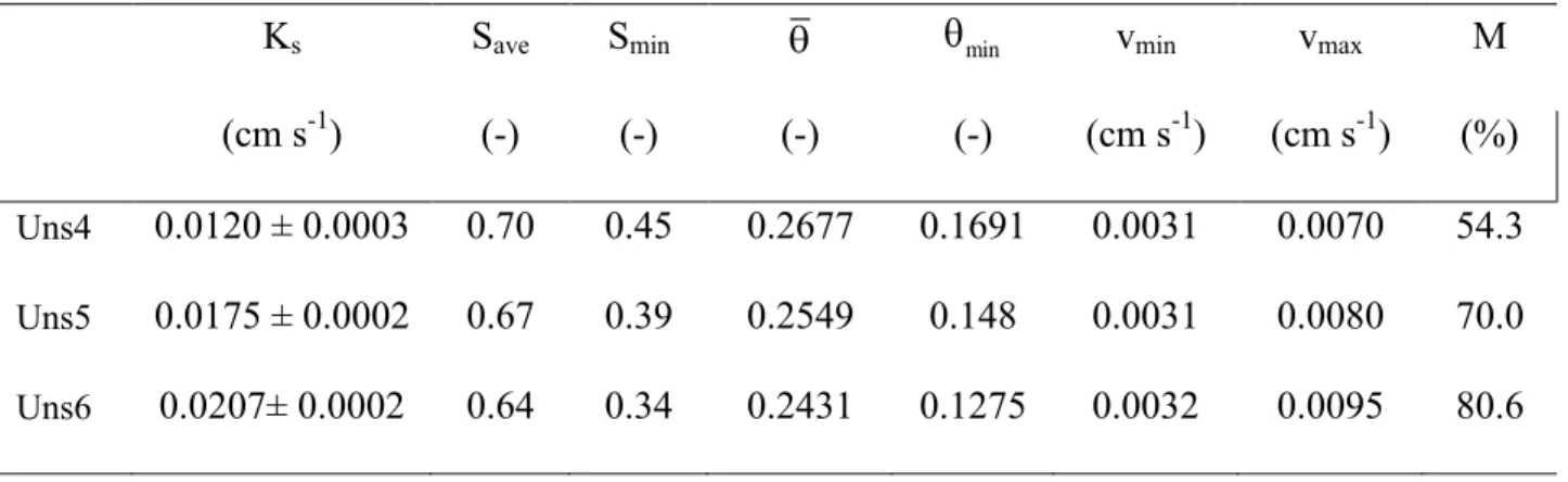
For each NP transport experiment, the hydrodynamic parameters estimated in Section 3.1 were applied to simulate the drainage of the column. The match between the measured and simulated cumulative outflows was quite poor. We assumed that these differences were due to column packing, which can be different from one experiment to another. We also assumed that the hydraulic conductivity was the most sensitive parameter because (i) it depends on the pore organization and pore connectivity, which can be packing dependent, and (ii) the experiments mainly consisted of gravitational drainage, and hydraulic conductivity is one of the most sensitive parameters under these conditions (Beydoun et al., 2006; Durner and Iden, 2011). Therefore, the saturated hydraulic conductivity was estimated by model calibration of the outflow during drainage (Table 1), and the other flow parameters remained unchanged. The

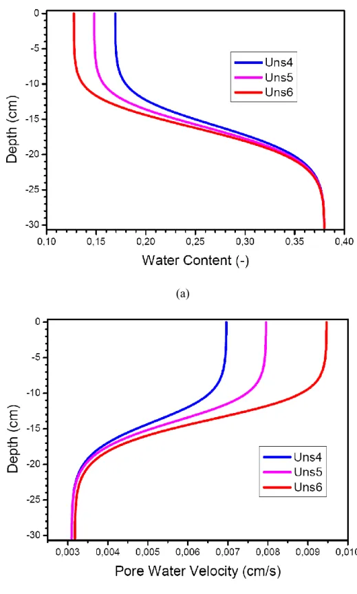
obtained hydraulic parameters were slightly different from one experiment to another (Table 1) and were consistent with previous works (Younes et al., 2013) as well as the value estimated using the Rosetta pedotransfer function (Schaap et al., 2001) calculation (0.016 cm/sec). Due to the boundary conditions of the experiment (prescribed flux at the top, prescribed pressure at the bottom), the differences in hydraulic conductivity led to different pressure distributions over the column and therefore different water content and water velocity profiles (Figure 2). During all experiments, the bottom of the column remained fully saturated (=0.38) and the water content decreased along the column profiles and reached the minimum at the column’s top. The different experiments had water content values of 0.13, 0.15 and 0.17, corresponding to 34%, 39% and 45% saturation at the column top, respectively. Because the pore water velocity is inversely proportional to the water content, the velocity profiles also showed small differences at the column top (from 0.007 cm/s to 0.009 cm/s) and the value increased until three times from the bottom to the top of the columns. These variations in the water content and pore water velocity along the column profiles and between the experiments originated from the small differences in the drainage processes (less than 5% for the cumulative drained water). This demonstrates the importance of accurate water flow modeling and the motivation for the development of an adapted model for NP retention in unsaturated porous media. It also underlines the difficulty of reproducing transport experiments under unsaturated conditions when sorption processes are linked to the water content and to the water velocity.

4.2 Breakthrough Curves

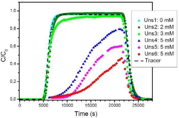
The column experiments were performed under four IS treatments (0-2-3-5 mM KCl). The transport of TiO2 NPs at 0 and 2 mM KCl did not show any NP retention. Instead, under 3 and 5

mM KCl, the BTCs showed a retention that increased as IS decreased (Figure 3). The experiments with an IS of 0, 2 and 3 mM were conducted at least in duplicate, whereas the experiments with an IS of 5 mM were repeated three times. The experiments with an IS of less than 5 mM KCl were reproducible, whereas the experiments with an IS equal to 5 mM KCl were not.

The NP behaved like a tracer for an IS of 0 mM and 2 mM, which made the experiments easily reproducible. Retention was observed for the experiment performed with an IS of 3 mM, and the experiments remained reproducible. Comparison with the BTCs obtained under saturated conditions, with an average fluid velocity of the same order of magnitude (0.002 cm/s in saturated condition, 0.003 cm/s in unsaturated condition), showed that similar retention processes occurred and that the effect of unsaturated conditions could be neglected for this IS (Figure 4). This interpretation agrees with the article of Fang (2009), where it is stated that decreasing the water saturation did not enhance the retention of TiO2 NP in sand columns.

The shapes of the 5 mM elution curves were typical of blocking behavior. This retention mechanism, resulting in an increase of the NP concentration over time during the elution, consisted of the progressive saturation of the attachment sites. Considering the unsaturated conditions in the 5 mM experiments, a fraction of the available attachment sites was probably positioned on the charged AWI. All of the BTC shapes were monotonic and showed a change in convexity. The data reported in Table 1 showed that the NP retention increased when the saturation decreased. Because the AWI was supposed to increase when the saturation decreased, this observation supports the assumption that NPs were retained from the AWI.

The set of partial differential equations (4-6), (9-12), (14-17) were solved numerically using discontinuous finite element method (Diaw et al., 2001) and a fully coupled implicit scheme. For the parameter estimation, the Levenberg-Marquardt method was adopted. The results of the calibrations of the different models are shown in Table 2. The value of the objective function (O) is reported for each calibration, i.e., the sum of quadratic differences between the measured and simulated concentrations after model calibration. The smaller O is, the better the fit is. It can be observed that the quality fit was better for the water content and water velocity dependent models with respect to the traditional 1S model. The BTC UNS6 could be described reasonably well by both the 1S_SWI and 1S_AWI models (O≈6×10-3) through two non-correlated parameters. Consequently, the two-site retention model 2S is not necessary to describe UNS6 because adding other parameters did not increase the quality of the fit, but only increased the correlation between the parameters. On the contrary, the 2S model considerably improved the fit quality of UNS4 and UNS5 compared to the one-site retention models. The objective function of the 2S fits is one order of magnitude smaller than the objective functions of the 1S_SWI and 1S_AWI model fits. The parameters a1swi, a1awi and pcawi are strongly correlated for UNS4 and

UNS5: To increase the quality of the fit, the number of parameters was reduced. In Equation 16, smaxawi, and thus a1awi, are assumed to be very large. Equation 16 can be reduced to (2S_INF)

AWI AWI a a s θk t c     (21)

This assumption reduces the number of parameters from four to three to calibrate the 2S model. This parameter reduction results in a small increase of the objective function and a decrease in the correlation between the parameters. The BTC prediction of the 1S and 2S_INF models can be found in Figure 5.

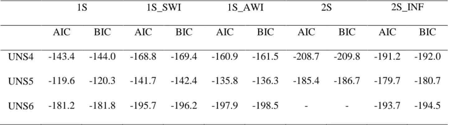
A better model fit does not suggest a better model performance when additional parameters are required. More information about the performance of the models can be obtained from a

comparison of the AIC and BIC criteria used for model discrimination (Burnham and Anderson 2002, Riva et al., 2011):

1

2

AIC 2 Log( / )

BIC Log( ) Log( / )

      p m m p m m m N N O N C N N N O N C (22)

where Np is the number of parameters, Nm is the number of measurements (53, 48, and 52 for

Uns4, Uns5, and Uns6, respectively), and O is the objective function. C1 and C2 are constants

that are set to zero because these criteria are used for model comparisons. The AIC and BIC criteria values for the 1S, 1S_SWI, 1S_AWI, 2S and 2S_INF models are compared in Table 3. It follows that the water content profile dependent models perform better than the 1S model. Moreover, the two-site models have a better performance than the one-site models for UNS4 and UNS5. As expected, the one-site models have better performances for UNS6. It can be observed that the assumption of a very large a1awi in the 2S model results in a small loss in model

performance and a reduction of the correlation between pcawi and a1sw (UNS4: from 0.986 to

-0.119; UNS5: from -0.992 to -0.951).

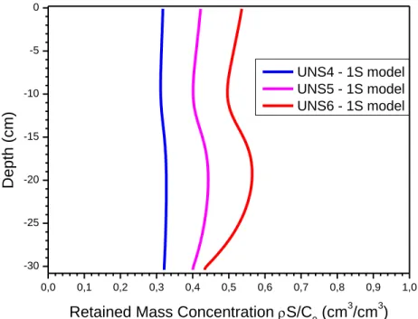
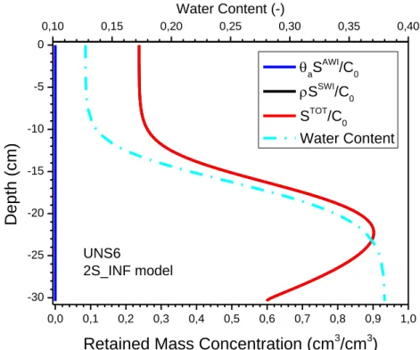
The predicted profiles of the retained concentrations of models 1S and 2S_INF are shown in Figure 6, and the profiles of ka and smax are shown in Figure 7. The retention profiles predicted

by the 1S model show two zones of ‘relatively’ higher retention: at the top of the column where the injected concentration is still high and at the transition zone defined by significant variations of the water content and therefore the velocity (at depths of approximately 15 to 20 cm – see Figure 6).

On the contrary, the shape of the retained NP for the 2S_INF model, that is, the sum the retention at the AWI and SWI, has a single maximum in the lower part of the column. The contribution of the AWI to the retention is significant but smaller than the SWI contribution. The attachment coefficient ka and amount of attachment sites smax vary along the column profile. The parameter

smaxawi increases with the water content, whereas kaawi and kaswi decrease from the top of the

column, where the water velocity is higher (Figure 2), to the bottom of the column.

6. Conclusions

In the TiO2 NP transport experiments under unsaturated conditions, the saturation profile

influenced the NP retention for an IS of 5 mM KCl, but not for lower IS. It can be deduced that under conditions of a lower IS, NPs are not retained at the interface between air and water. This is an interesting issue because in the literature it is not clear whether the interface between air and water can retain NPs or not.

The 2S model developed in this article describes the retention of NPs as a function of the water content and water velocity. It can be used for both saturated and unsaturated conditions and for a rather large range of velocities. Furthermore, it directly takes into account the retention on the interface between air and water. However, it is still limited to an ionic strength of 5 mM. The 2S model offers a better description of the BTCs than that issued from a direct optimization of the retention parameters (1S model). The 2S model predicts lower NP retention at the unsaturated zones of the column profiles compared to the 1S predictions. The retention profile measurements were not performed, and thus, the retention profile predictions of the 2S model were not

Acknowledgments

This work was funded by the MESONNET project supported by the French National Research Agency – Nanotechnoly and Nanosystems-2010 program.

References

Abbaspour, K.C., Schulin, R., van Genuchten, M.Th., 2001. Estimating unsaturated soil hydraulic parameters using ant colony optimization. Advances in Water Resources 24(8), 827-841.

Adam, V., Loyaux-Lawniczak, S., Quaranta, G., 2015. Characterization of engineered TiO2 nanomaterials in a life cycle and risk assessments perspective. Environmental Science and Pollution Research 22(15), 11175-11192.

Anders, R., Chrysikopoulos, C.V., 2009. Transport of viruses through saturated and unsaturated columns packed with sand. Transport in Porous Media 76(1), 121-138.

Beydoun, H., Lehmann, F., 2006. Drainage experiments and parameter estimation in unsaturated porous media. Comptes Rendus – Geoscience 338(3), 180-187.

Bradford, S. A., Simunek, J., Bettahar, M., van Genuchten, M. T., Yates, S. R., 2006. Significance of straining in colloid deposition: Evidence and implications. Water Resources Research 42(12), W12S15.

Bradford, S.A. , Torkzaban, S., 2008. Colloid transport and retention in unsaturated porous media: A review of interface-, collector-, and pore-scale processes and models. Vadose Zone Journal 7(2), 667-681.

Burnham, K.P., Anderson D.R., 2002. Model selection and multimodel inference: a practical information – theoretic approach. 2nd edition, Springer, 488p.

Chen, L., Sabatini, D.A., Kibbey, T.C.G., 2008. Role of the air-water interface in the retention of TiO2 nanoparticles in porous media during primary drainage. Environmental Science &

Chen, L., Sabatini, D.A., Kibbey, T.C.G., 2010. Retention and release of TiO 2 nanoparticles in unsaturated porous media during dynamic saturation change. Journal of Contaminant Hydrology 118(3-4), 199-207.

Corapcioglu, M.Y., Choi, H., 1996. Modeling colloid transport in unsaturated porous media and validation with laboratory column data. Water Resources Research 32(12), 3437-3449.

De Novio, N.M., Saiers, J.E., Ryan, J.N., 2004. Colloid movement in unsaturated porous media: Recent advances and future directions. Vadose Zone Journal 3(2), 338-351.

Diaw, E.B., Lehmann, F., Ackerer, Ph., 2001. One-dimensional simulation of solute transfer in saturated-unsaturated porous media using the discontinuous finite elements method. Journal of Contaminant Hydrology, 51(3-4)197-213.

Durner, W., and S. C. Iden 2011. Extended multistep outflow method for the accurate determination of soil hydraulic properties near water saturation, Water Resources Research, 47(8), W08526.

Emmanuel, S., Berkowitz, B., 2005. Mixing-induced precipitation and porosity evolution in porous media. Advances in Water Resources 28(4), 337-344.

Fang, J., Xu, M.J., Wang, D.J., Wen, B., Han, J.Y., 2013. Modeling the transport of TiO2

nanoparticle aggregates in saturated and unsaturated granular media: effects of ionic strength and pH. Water Research 47(3), 1399 – 1408.

Hayek, M., Lehmann, F., Ackerer, P., 2008. Adaptive multi-scale parameterization for one-dimensional flow in unsaturated porous media. Advances in Water Resources 31(1), 28-43. Knappenberger, T., Aramrak, S., Flury, M., 2015. Transport of barrel and spherical shaped colloids in unsaturated porous media. Journal of Contaminant Hydrology, 180, 69-79. Kumahor, S.K., Hron, P., Metreveli, G., Schaumann, G.E., Vogel, H.J., 2015. Transport of citrate-coated silver nanoparticles in unsaturated sand. Science of The Total Environment 535, 113–121.

Lenhart, J.J., Saiers, J.E., 2002. Transport of silica colloids through unsaturated porous media: Experimental results and model comparisons. Environmental Science & Technology 36(4), 769-777.

Liang, Y., Bradford, S.A., Simunek, J., Heggen, M., Vereecken, H., Klumpp, E., 2013a.

Retention and remobilization of stabilized silver nanoparticles in an undisturbed loamy sand soil. Environmental Science and Technology 47(21), 12229-12237.

Liang, Y., Bradford, S.A., Simunek, J., Vereecken, H., Klumpp, E., 2013b. Sensitivity of the transport and retention of stabilized silver nanoparticles to physicochemical factors. Water Research 47(7), 2572 – 2582.

Pinder, G. F., Celia, M. A., 2006. Subsurface hydrology. John Wiley & Sons, 488p.

Riva, M., Panzeri, M., Guadagnini, A., Neuman, S.P., 2011. Role of model selection criteria in geostatistical inverse estimation of statistical data- and model- parameters. Water Resources Research 47(7), W07502.

Ryan, J.N., Elimelech, M., 1996. Colloid mobilization and transport in groundwater. Colloids and Surfaces A: Physicochemical and Engineering Aspects 107, 1-56.

Schaap, M. G., Leij, F. J., van Genuchten, M. T., 2001. ROSETTA: a computer program for estimating soil hydraulic parameters with hierarchical pedotransfer functions. Journal of hydrology 251, 163–176.

Solovitch, N., Labille, J., Rose, J., Chaurand, P., Borschneck, D., Wiesner, M.R., Bottero, J.-Y., 2010. Concurrent aggregation and deposition of TiO2 nanoparticles in a sandy porous media. Environmental Science & Technology 44(13), 4897–4902.

Syngouna, V. I., Chrysikopoulos, C.V., 2015. Experimental investigation of virus and clay particles cotransport in partially saturated columns packed with glass beads. Journal of Colloid and Interface Science, 440, 140-150.

Toloni, I., 2015. Transport of TiO2 nanoparticles in saturated and unsaturated porous media: experiments and modeling. PhD thesis, University of Strasbourg.

https://www.theses.fr/2015STRAH018/document, 145p.

Toloni, I., Lehmann, F., Ackerer, P., 2014. Modeling the effects of water velocity on TiO2 nanoparticles transport in saturated porous media. Journal of Contaminant Hydrology 171, 42– 48.

Tufenkji, N., Elimelech, M., 2004. Correlation Equation for Predicting Single-Collector Efficiency in Physicochemical Filtration in Saturated Porous Media. Environmental Science & Technology 38(2), 529–536.

Wollschläger, U., Pfaff, T., Roth, K., 2009. Field-scale apparent hydraulic parameterisation obtained from TDR time series and inverse modelling. Hydrology and Earth System Sciences 13(10), 1953–1966.

Ye, M., Meyer, P.D., Neuman, S.P., 2008. On model selection criteria in multimodal analysis. Water Resources Research 44(3), W03428.

Younes, A., Mara, T., Fajraoui, N., Lehmann, F., Belfort, B., Beydoun, H, 2013. Use of global sensitivity analysis to help assess unsaturated soil hydraulic parameters. Vadose Zone Journal 12(1), 1–12.

Zhang, Qiulan, Hassanizadeh, S.M., Raoof, A., van Genuchten, M. Th., Roels, S.M., 2012. Modeling virus transport and remobilization during transient partially saturated flow. Vadose Zone Journal 11(2), 1–11.

Figure 1: Pressure head measurements (dots) during the step by step drainage and modeling results (line).

(a)

(b)

Figure 2: Modeled water content profiles (a) and pore water velocity profiles (b) for the 5 mM unsaturated nanoparticles transport experiments.

Figure 3: Breakthrough curves of the unsaturated transport experiments with TiO2 nanoparticles

under 0-2-3-5 mM KCl and with a conservative tracer.

Figure 4: BTCs of the 3 mM unsaturated transport experiment superposed to a 3 mM saturated experiment (injection of 2.5 VP (resp. 3VP) for the unsaturated (resp. saturated) experiment).

0 5000 10000 15000 20000 25000 0,0 0,2 0,4 0,6 0,8 1,0 C/ C 0 Time (s) Uns4 Uns5 Uns6 Uns4 - 1S Uns5 - 1S Uns6 - 1S Tracer (a) 0 5000 10000 15000 20000 25000 0,0 0,2 0,4 0,6 0,8 1,0 C/ C 0 Time (s) Uns4 Uns5 Uns6 Uns4 - 2S_INF Uns5 - 2S_INF Uns6 - 2S_INF Tracer (b)

Figure 5: Breakthrough curves of the unsaturated transport experiments modeled by the 1S model (a) and by the 2S_INF model (b).

0,0 0,1 0,2 0,3 0,4 0,5 0,6 0,7 0,8 0,9 1,0 -30 -25 -20 -15 -10 -5 0 De pt h (cm)

Retained Mass Concentration S/C

0 (cm 3 /cm3) UNS4 - 1S model UNS5 - 1S model UNS6 - 1S model (a)

0,00 0,05 0,10 0,15 0,20 0,25 0,30 0,35 0,40 -30 -25 -20 -15 -10 -5 0 De pth (cm)

Retained Mass Concentration (cm3/cm3) _aSAWI/C₀ SSWI/C₀ STOT/C₀ Water Content 0,10 0,15 0,20 0,25 0,30 0,35 0,40 Water Content (-) UNS4 2S_INF model (b) 0,00 0,05 0,10 0,15 0,20 0,25 0,30 0,35 0,40 -30 -25 -20 -15 -10 -5 0 De pth (cm)

Retained Mass Concentration (cm3/cm3) _aSAWI/C₀ SSWI/C₀ STOT/C₀ Water Content 0,10 0,15 0,20 0,25 0,30 0,35 0,40 Water Content (-) UNS5 2S_INF model (c)

0,0 0,1 0,2 0,3 0,4 0,5 0,6 0,7 0,8 0,9 1,0 -30 -25 -20 -15 -10 -5 0 De pth (cm)

Retained Mass Concentration (cm3/cm3) _aSAWI/C₀ SSWI/C₀ STOT/C₀ Water Content 0,10 0,15 0,20 0,25 0,30 0,35 0,40 Water Content (-) UNS6 2S_INF model (d)

Figure 6: Retention profiles of the 5 mM NP transport experiments modeled by the 1S (a) and 2S_INF models (b, c, d).

2,5 3,0 3,5 4,0 4,5 5,0 5,5 6,0 6,5 -30 -25 -20 -15 -10 -5 0 2S_INF model De pth (cm) kSWI_a (10-4 s-1) UNS4 UNS5 UNS6 (a) 0,0 0,1 0,2 0,3 0,4 0,5 0,6 0,7 0,8 0,9 1,0 1,1 -30 -25 -20 -15 -10 -5 0 2S_INF model De pth (cm) SSWI_max/C₀ (cm3/cm3) UNS4 UNS5 UNS6 (b)

0,00 0,02 0,04 0,06 0,08 0,10 0,12 -30 -25 -20 -15 -10 -5 0 2S_INF model De pth (cm) kAWI_a (10-4 s-1) UNS4 UNS5 UNS6 (c)

Figure 7: Profiles of the parameters ka and smax related to the interface between sand and water (a, b) and to the interface between air and water (c). Parameters of the 2S_INF model by

Table 1: Measured and modeled parameters of the unsaturated transport experiments*.

Ks Save Smin  min vmin vmax M

(cm s-1) (-) (-) (-) (-) (cm s-1) (cm s-1) (%)

Uns4 0.0120 ± 0.0003 0.70 0.45 0.2677 0.1691 0.0031 0.0070 54.3

Uns5 0.0175 ± 0.0002 0.67 0.39 0.2549 0.148 0.0031 0.0080 70.0

Uns6 0.0207± 0.0002 0.64 0.34 0.2431 0.1275 0.0032 0.0095 80.6

*Errors represent the 95% confidence interval. Ks is the optimized saturated hydrodynamic saturation; Save/min is the average and minimum values of the modeled local saturation; is the average and minimum values of the modeled water content; vmin/max is the maximum and minimum values of the modeled pore water velocity; M is percentage of NP mass retained from the porous medium.

Table 2: Optimized parameters of the retention models 1S, 1S_SWI, 1S_AWI, 2S and 2S_INF*. smax/C0 (cm3 _cm-3₎ ka (× 10-4 _s-1₎ O (×10-3₎ Uns4 0.33 ± 0.01 3.9 ± 0.2 87.5 1S Uns5 0.47 ± 0.02 4.7 ± 0.4 127.7 Uns6 0.60 ± 0.01 6.3 ± 0.2 14.2 a1swi (g g-1₎ pcswi (-) a1awi (g cm-3₎ pcawi (-) O (×10-3₎ Uns4 5.36 ± 0.01 0.073 ± 0.057 - - 29.09 1S_SWI Uns5 7.92 ± 0.22 0.091 ± 0.008 - - 44.20 Uns6 11.12 ± 0.16 0.127 ± 0.006 - - 7.518 Uns4 - - 163.32 ± 3.88 1.967 ± 0.131 40.96 1S_AWI Uns5 - - 176.32 ± 5.29 1.988 ± 0.175 59.07 Uns6 - - 191.14 ± 2.25 2.259 ± 0.081 6.813 Uns4 0.908 ± 0.213 0.071 ± 0.008 148.79 ± 4.62 1.172 ± 0.150 40.96 2S Uns5 1.37 ±  0.132 ± 0.015 180.19 ± 5.65 0.972 ± 0.169 59.07 Uns6 - - - Uns4 3.855± 0.005 0.089 ± 0.006 - 0.121 ± 0.338 40.96 2S_INF Uns5 3.573 ± 0.159 0.143 ± 0.01 - 0.285 ± 0.016 59.07 Uns6 11.12 ± 6.77 0.128 ± 0.009 - 3.0 10-8 _{± 0.24 6.813}

*Errors represent the 95% confidence interval. smax/C0 and ka are 1S model parameters; a1swi

Table 3: AIC and BIC criteria for the 1S, 1S_SWI, 1S_AWI, 2S and 2S_INF models.

1S 1S_SWI 1S_AWI 2S 2S_INF

AIC BIC AIC BIC AIC BIC AIC BIC AIC BIC

UNS4 -143.4 -144.0 -168.8 -169.4 -160.9 -161.5 -208.7 -209.8 -191.2 -192.0 UNS5 -119.6 -120.3 -141.7 -142.4 -135.8 -136.3 -185.4 -186.7 -179.7 -180.7 UNS6 -181.2 -181.8 -195.7 -196.2 -197.9 -198.5 - - -193.7 -194.5