HAL Id: hal-00317560
https://hal.archives-ouvertes.fr/hal-00317560
Submitted on 7 Sep 2004
HAL is a multi-disciplinary open access
archive for the deposit and dissemination of
sci-entific research documents, whether they are
pub-lished or not. The documents may come from
teaching and research institutions in France or
abroad, or from public or private research centers.
L’archive ouverte pluridisciplinaire HAL, est
destinée au dépôt et à la diffusion de documents
scientifiques de niveau recherche, publiés ou non,
émanant des établissements d’enseignement et de
recherche français ou étrangers, des laboratoires
publics ou privés.
densities, and electron and ion temperatures in the
low-latitude ionosphere during 19-21 March 1988
A. V. Pavlov, S. Fukao, S. Kawamura
To cite this version:
A. V. Pavlov, S. Fukao, S. Kawamura. Comparison of the measured and modeled electron densities,
and electron and ion temperatures in the low-latitude ionosphere during 19-21 March 1988. Annales
Geophysicae, European Geosciences Union, 2004, 22 (8), pp.2747-2763. �hal-00317560�
SRef-ID: 1432-0576/ag/2004-22-2747 © European Geosciences Union 2004
Annales
Geophysicae
Comparison of the measured and modeled electron densities, and
electron and ion temperatures in the low-latitude ionosphere during
19–21 March 1988
A. V. Pavlov1, S. Fukao2, and S. Kawamura3
1Institute of Terrestrial Magnetism, Ionosphere and Radio-Wave Propagation, Russian Academy of Science (IZMIRAN),
Troitsk, Moscow Region, 142 190, Russia
2Radio Science Center for Space and Atmosphere, Kyoto University, Kyoto, 611-0011, Japan
3National Institute of Information and Communications Technology, 4-2-1, Nukui-kita, Koganei, Tokyo 184-8795, Japan
Received: 19 September 2003 – Revised: 9 March 2004 – Accepted: 30 March 2004 – Published: 7 September 2004
Abstract. We have presented a comparison between the
modeled NmF2 and hmF2, and NmF2 and hmF2 which were observed at the equatorial anomaly crest and close to the ge-omagnetic equator simultaneously by the Akita, Kokubunji, Yamagawa, Okinawa, Chung-Li, Manila, Vanimo, and Dar-win ionospheric sounders and by the middle and upper atmo-sphere (MU) radar at Shigaraki (34.85◦N, 136.10◦E, Japan) during the 19–21 March 1988 geomagnetically quiet time pe-riod at moderate solar activity near approximately the same geomagnetic meridian of 201◦. A comparison between the electron, Te, and ion, Ti, temperatures measured by the MU
radar and those produced by the model of the ionosphere and plasmasphere is presented for 19–21 March 1988. It is shown that there is a large disagreement between the measured and modeled hmF2 from about 07:00 UT to about 11:00 UT if the equatorial E×B drift given by Scherliess and Fejer (1999) is used. The required equatorial upward E×B drift is weaker from 03:14 UT to 11:14 UT than that given by Scherliess and Fejer (1999) for the studied time period. The required mod-ification of the E×B drift weakens the effect of the foun-tain in NmF2 bringing the modeled and measured hmF2 and NmF2, into reasonable agreement. The depth of the equa-torial NmF2 trough in the calculated NmF2 is approximately consistent with the measured depth if the modified equatorial E×B drift is used. It has been found that the north-south asymmetries in the observed NmF2 and hmF2 about the geo-magnetic equator are mainly caused by the asymmetry in the neutral wind about the geomagnetic equator. In the North-ern Hemisphere, the meridional neutral wind taken from the HWW90 wind model and the NRLMSISE-00 atomic oxygen density are corrected so that the model results agree with the ionospheric sounders and MU radar observations. A theory of the primary mechanisms causing the latitude dependence of the morning and evening peaks in Te is developed. The
latitude dependence of the magnitudes of these peaks in Te Correspondence to: A. V. Pavlov
(pavlov@izmiran.rssi.ru)
is interpreted in terms of the corresponding dependence of the electron density. The relative role of the E×B drift and the plasma drift caused by the neutral wind in the formation and the dependence of the magnitudes of the morning and evening electron temperature peaks on the geomagnetic lati-tude is studied.
Key words. Ionosphere (equatorial ionosphere; electric
fields and currents; plasma temperature and density; ionosphere-atmosphere interactions; modeling and forecast-ing)
1 Introduction
The ionosphere at the geomagnetic equator and low geomag-netic latitudes has been studied observationally and theoret-ically for many years (see review papers presented by Mof-fett, 1979; Anderson, 1981; Walker, 1981; Bailey and Balan, 1996; Rishbeth, 2000; Abdu, 1997, 2001, and references therein). The low-latitude ionosphere undergoes dramatic changes as a result of changes in plasma motion perpendic-ular to the geomagnetic field, B, due to an electric field, E, which is generated in the E-region. This electric field af-fects F-region plasma, causing both ions and electrons to drift in the same direction with a drift velocity, VE=E×B /B2. The zonal component of VE (geomagnetic east-
geo-magnetic west component) is thought to have only a negli-gible effect on the low-latitude plasma densities (Anderson, 1981), but changes in the meridianal component (component in the plane of a geomagnetic meridian) of the E×B drift velocity, caused by changes in the zonal component, E3, of
the electric field, affect the distribution of plasma in the low-latitude ionospheric F-region. The examination of the model of the meridional component of the drift velocity has been driven by the relationship between E3 and the dynamics of
the F2-layer close to the geomagnetic equator. It is shown by Pavlov (2003) that the agreement between the measured
and modeled F2-peak altitudes, hmF2, of the low-latitude ionosphere requires the correction of the empirical vertical drift model of Scherliess and Fejer (1999). The present work continues the study of the relationship between E3and the
dynamics of the low-latitude F2-layer in the present case study, in which NmF2 and hmF2 are observed simultane-ously close to the same geomagnetic meridian at the geomag-netic longitudes of 2010 ±11◦by the Akita, Kokubunji, Yamagawa, Okinawa, Chung-Li, Manila, Vanimo, and Dar-win ionospheric sounders and by the middle and upper atmo-sphere (MU) radar at Shigaraki (34.85◦N, 136.10◦E, Japan) during the 19–21 March 1988 geomagnetically quiet time pe-riod at moderate solar activity.
The importance of diffusion, electrodynamic drift, and neutral wind on the generation and modulation of the equa-torial anomaly in the electron density, Ne, the plasma
foun-tain and several founfoun-tain related features (an additional layer, a reverse fountain, an equatorial anomaly in vertical iono-spheric electron content, a noon bite-out in NmF2, a night-time increase in Ne, plasma bubbles and spread F) were
stud-ied by Balan and Bailey (1995) and Balan et al. (1997a). In the present work, we investigate the equatorial anomaly characteristics (the equatorial trough, and crest latitudes and magnitudes) from the comparison between the measured and modeled Ne and electron temperatures, Te, during 19–21
March 1988, using the new two-dimensional time depen-dent model of the low- and middle-latitude plasmasphere and ionosphere (Pavlov, 2003), which employs the updated rate coefficients of chemical reactions of ions and the updated N2,
O2, and O photoionization and photoabsorption cross
sec-tions. The horizontal neutral wind drives the low-latitude F-layer plasma along magnetic field lines and causes significant north–south asymmetry in the equatorial ionization anomaly, producing notable effects on spread F generation and dynam-ics, and resulting in longitude dependent seasonal variabil-ity of Ne (Rishbeth, 1972, 2000; Balan and Bailey, 1995;
Balan et al., 1997a, b; Abdu, 1997, 2001). We investigate the role of horizontal neutral winds in the ionization distribu-tion, plasma dynamics, structuring, and thermal balance of the low-latitude ionosphere in the plane of the geomagnetic meridian of 201◦during 19–21 March 1988.
Ionospheric models are particularly valuable for investi-gating the changes that would result in observed quantities from changes in individual input parameters. The model of the ionosphere and plasmasphere of Pavlov (2003) uses the neutral temperature and densities as the model input. As a result, model/data discrepancies can arise due to a possible inability of the neutral atmosphere model to accurately pre-dict the thermospheric response to the studied time period in the upper atmosphere. We investigate how well the MU radar data and the Akita, Kokubunji, Yamagawa, Okinawa, Chung-Li, Manila, Vanimo, and Darwin ionospheric sounder measurements of NmF2 taken during the 19–21 March 1988 geomagnetically quiet period agree with those calculated by the model of the ionosphere and plasmasphere using the NRLMSISE-00 model neutral temperature and densities given by Picone et al. (2002).
It follows from the electron, Te, and ion, Ti, temperature
profiles measured at Jicamarca that the enlargement of the altitude region with Te>Ti occurs at sunrise at all heights
to at least 600 km (McClure, 1969). The diurnal variation of the low-latitude Te is characterized by a morning peak
(McClure, 1971; Oyama et al., 1996) and an evening peak (Fukao et al., 1991; Watanabe and Oyama, 1997). It is shown by Oyama et al. (1996) that the latitude dependence of the morning peak in Te at 600 km for the June solstices at
so-lar maximum is caused by the electron density latitude de-pendence due to a downward E×B plasma drift. Otsuka et al. (1998) found that the occurrence and strength of the morn-ing and evenmorn-ing peaks in Te over the MU radar depend on
altitude, season, and solar activity under magnetically quiet conditions during 1986–1995. However, Otsuka et al. (1998) presented only a typical average picture of the diurnal elec-tron temperature variations over the MU radar and did not compare the measured and modeled Te over the MU radar
for a specific time period. In this work, we study the latitude dependence of the occurrence and strength of the morning and evening peaks in Teand the mechanisms causing these
peaks in the low-latitude ionosphere during geomagnetically quiet time conditions of 19–21 March 1988 at moderate so-lar activity. The reliability of the conclusions is based on the comparison between the measured MU radar and modeled Te, and the use of the updated electron cooling rates (Pavlov,
1998 a, b; Pavlov and Berrington, 1999) in the model.
2 Theoretical model
The model of the low- and middle-latitude ionosphere and plasmasphere, which is described in detail by Pavlov (2003), calculates number densities, Ni, of O+(4S), H+, NO+, O+2,
N+2, O+(2D), O+(2P), O+(4P), and O+(2P*) ions, N
e, Te,
and Ti. As the model inputs, the horizontal components of
the neutral wind are specified using the HWW90 wind model (Hedin et al., 1991), the model solar EUV fluxes are taken from the EUVAC model (Richards et al., 1994), while neutral densities and temperature are taken from the NRLMSISE-00 model (Picone et al., 2002).
Dipole orthogonal curvilinear coordinates q, U, and 3 are used in the model calculations, where q is aligned with, and U and 3 are perpendicular to, the magnetic field, and the U and 3 coordinates are constant along a dipole magnetic field line. It should be noted that q=(RE/R)2cos 2, U=(RE/R)
sin2 2, and 3 is the geomagnetic longitude, where R is the radial distance from the Earth’s center, 2=900−ϕ is the geomagnetic colatitude, ϕ is the geomagnetic latitude, REis
the Earth’s radius. In the model,VE=VE3e3+VEU eU, where
VE
3=EU/B is the zonal component of VE, VEU= -E3/B is the
meridional component of VE, E =E3e3+EU eU, E3is the
3(zonal) component of E in the dipole coordinate system, EU is the U (meridional) component of E in the dipole
coor-dinate system, e3and eU are unit vectors in 3 and U
direc-tions, respectively, eU is directed downward at the
Equations which determine the trajectory of the iono-spheric plasma perpendicular to magnetic field lines and the moving coordinate system are derived by Pavlov (2003). The effects of the zonal (geomagnetic east-geomagnetic west) component of the E×B drift on Ni, Ne, Te, and Ti are
not taken into account in the model calculations (Anderson, 1981). It means that the model works as a time dependent two-dimensional (q and U coordinates) model of the iono-sphere and plasmaiono-sphere. In this approximation, the trajec-tory of the ionospheric plasma in the U direction is found from the equation (Pavlov, 2003)
∂ ∂tU =−E eff 3R −1 E B −1 0 , (1)
where Eeff3= E3h3R−E1 , h3=R sin 2, B0 is the equatorial
value of B for R=REand 2=0.
The value of Eeff3 is not changed along magnetic field lines, because the model takes into account that the magnetic field lines are “frozen” in the ionospheric and plasmaspheric plasma (Pavlov, 2003):
∂ ∂q(E
eff
3)=0. (2)
It should be noted that Eqs. (1)-(2) determine the changes in E3along magnetic field lines and the altitude dependence of
E3in the ionosphere and plasmasphere.
In the model of the ionosphere and plasmasphere, the de-pendence of E3 on the solar local time, tge, over the
ge-omagnetic equator given by the dash-dotted line in Fig. 1 is obtained from the empirical F-region quiet time equato-rial vertical drift velocity presented in Fig. 8 of Scherliess and Fejer (1999) for equinox conditions. As it will be dis-cussed later in Sect. 4.1, this empirical equatorial zonal elec-tric field is modified in the time range between 12:00 SLT and 24:00 SLT by the use of the comparison between the measured and modeled values of hmF2, where SLT is the solar local time at the geomagnetic equator for the geomag-netic longitude of 201◦. The resulting equatorial magnitude of E3(tge), which is used in the model calculations, is shown
by the solid line in Fig. 1. It should be noted that the pro-cedure used to correct the E×B drift (comparing measured and modeled hmF2) is the same as that used by Balan et al. (1996). There are no MU radar vertical drift velocity measurements for the studied time period. We take into ac-count that the perpendicular drifts over Arecibo and the MU radar for solstice seasons are similar (Takami et al., 1996). Therefore, the average quiet time value of E3at the F-region
altitudes over Arecibo (dashed line in Fig. 1) is found from Fig. 2 of Fejer (1993), where the average quiet time perpen-dicular/northward F-region plasma drift for equinox condi-tions is presented and assumed to be similar to the value of E3above the MU radar.
Equations (1–2) determine the trajectory of the iono-spheric plasma perpendicular to magnetic field lines and the moving coordinate system. It follows from Eq. (1) that time variations of U caused by the existence of the E3
compo-nent of the electric field are determined by time variations of
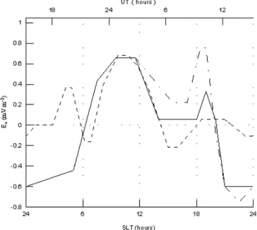
Fig. 1. Diurnal variations of E3during each day of 17–21 March
1988. The empirical F-region quiet time vertical drift velocity over the geomagnetic equator presented in Figure 8 of Scherliess and Fe-jer (1999) for equinox conditions was used for the equatorial value of E3(dash-dotted line). The solid line shows the empirical
equa-torial electric field, which was modified in the time range between 12:00 SLT and 24:00 SLT by the use of the comparison between the measured and modeled hmF2. The dash-dotted line coincides with the solid line between 00:00 SLT and 12:00 SLT. The average quiet time value of E3 at the F-region altitudes over Arecibo (dashed
line) is found from the average quiet time perpendicular/northward F-region plasma drifts for equinox conditions presented in Fig. 2 of Fejer (1993). SLT is the local solar time at the geomagnetic equator and 201◦geomagnetic longitude.
Eeff3. We have to take into account Eq. (2), which shows that magnetic field lines are “frozen” in the ionospheric plasma. As a result, Eeff3(t) is not changed along magnetic field lines. The equatorial and Arecibo values of E3(tge)are used to find
the equatorial and Arecibo values of Eeff3(tge)from Eq. (2).
The equatorial value of Eeff3(tge)is used for magnetic field
lines with an apex altitude, hap=Req-RE, less than 600 km,
where Req is the equatorial radial distance of the magnetic
field line from the Earth’s center and REis the Earth’s radius.
The Arecibo value of Eeff3(tge)is used if the apex altitude is
greater than 2126 km. Linear interpolation of the equatorial and Arecibo values of Eeff3(tge)is employed at intermediate
apex altitudes.
The model calculates Ni, Ne, Ti, and Tein the fixed nodes
of the fixed volume grid. This Eulerian computational grid consists of a distribution of the dipole magnetic field lines in the ionosphere and plasmasphere. One hundred dipole mag-netic field lines are used in the model for each fixed value of 3. The number of the fixed nodes taken along each mag-netic field line is 191. For each fixed value of 3, the region of study is a (q,U) plane, which is bounded by two dipole magnetic field lines. The low boundary magnetic field line
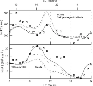
Fig. 2. Observed (squares) and calculated (lines) hmF2 (top panel)
and NmF2 (bottom panel) on 19 March 1988. The model calcu-lations have been carried out with different combinations of the model input parameters. The combinations are 1) the SF E3, given
by das-dotted line in Fig. 1, the NRLMSISE-00 neutral tempera-ture and densities, and the HWW90 wind (dotted curves), 2) the SF E3, the NRLMSISE-00 neutral temperature and densities, and the zero neutral wind (dashed curves), 3) the modified E3, given
by solid line in Fig. 1, the NRLMSISE-00 neutral temperature and densities, and the HWW90 wind (dash-dot curves), and 4) the cor-rected equatorial E3, given by solid line in Fig. 1, the
NRLMSISE-00 neutral temperature and densities with the corrected value of [O], and the corrected HWW90 wind (solid curves). The correc-tions of the NRLMSISE-00 [O] and the HWW90 wind, are used to make the measured and modeled NmF2 and hmF2 agree over the MU radar and over all the ionosonde stations in Table 1. The NRLMSISE-00 model [O] was increased by a factor of 1.5 in the 0–15◦geomagnetic latitude range of the Northern Hemisphere from 05:14 UT to 09:44 UT. The meridional neutral wind, W, of the Northern Hemisphere, taken from the HWW90 wind model, was changed to W+1W, where 1W=-30 m/sec−1between 10:14 UT and 13:44 UT during 17–21 March 1988, 1W=30 m/sec−1from 15:14 UT to 24:00 UT and from 00:00 UT to 00:14 UT during 17– 21 March 1988, 1W=20 m sec−1from 01:14 UT to 06:14 UT on 21 March 1988, and 1W=0 from 00:14 UT to 09:14 UT during 17–21 March 1988 and from 07:14 UT to 09:14 UT on 21 March 1988. A linear interpolation between the values of 1W was used in the intermediate time periods. These values of 1W are used above the geomagnetic latitude of 24◦, while 1W=0 at the geomagnetic equator. A square interpolation of 1W is employed between 24◦ and 0◦.
has hap=150 km. The upper boundary magnetic field line
has hap=4491 km and intersects the Earth’s surface at two
middle-latitude geomagnetic latitudes: ±40◦. The computa-tional grid dipole magnetic field lines are distributed between these two boundary lines. They have the interval, 1hap, of
20 km between hap of the low boundary line and hp of the
nearest computational grid dipole magnetic field line. The value of 1hap is increased from 20 km to 45 km linearly as
we go from the low computational grid boundary line to the upper computational grid dipole magnetic field line. We ex-pect our finite-difference algorithm, which is described be-low, to yield approximations to Ni, Ne, Ti, and Te in the
ionosphere and plasmasphere at discrete times t=0, 1t, 21t, with the time step 1t=10 min. The model starts at 05:14 UT on 17 March. This UT corresponds to 14:00 SLT at the ge-omagnetic equator and 201◦ geomagnetic longitude. The model is run from 05:14 UT on 17 March 1988 to 24:00 UT on 18 March 1988 before model results are used.
3 Solar geophysical conditions and data
The value of the geomagnetic Kp index was between 0 and
2+for most of the studied time period of 19–21 March 1988,
except between 09:00 and 12:00 UT on 20 March when the magnitude of Kp was 3+. It should be noted that when the
thermosphere is disturbed it takes time for it to relax back to its initial state, and this thermospheric relaxation time de-termines the time for the disturbed ionosphere to relax back to the quiet state. It means that not every time period with Kp≤3 can be considered as a magnetically quiet time
pe-riod. The characteristic time of the neutral composition re-covery after a storm impulse event ranges from 7 to 12 h, on average (Hedin, 1987), while it may need up to days for all altitudes down to 120 km in the atmosphere to recover completely back to the undisturbed state of the atmosphere (Richmond and Lu, 2000). The value of Kpwas between 0
and 30for the previous 17–18 March 1988 time period, i.e.
the studied time period of 19–21 March 1988 can be consid-ered as a quiet time period. The F10.7 solar activity index was 116–118, while the 81-day averaged F10.7 solar activity index was 107.
The middle and upper atmosphere (MU) radar at Shi-garaki, which is located at the geomagnetic latitude of 24.5◦ and the geomagnetic longitude of 203.2◦, operated from 00:00 SLT on 19 March to 07:00 SLT on 22 March. The ca-pabilities of the radar for incoherent scatter observations have been described and compared with those of other incoherent scatter radars by Sato et al. (1989) and Fukao et al. (1990). Rishbeth and Fukao (1995) reviewed the MU radar studies of the ionosphere and thermosphere. The data that we use in this work are the measured time variations of altitude profiles of the electron density and temperature, and the ion temper-ature between 200 km and 600 km over the MU radar.
We use hourly critical frequencies, fof2 and foE, of the F2 and E layers, and maximum usable frequency param-eter, M(3000)F2, data from the Akita, Kokubunji, Yama-gawa, Okinawa, Chung-Li, Manila, Vanimo, and Darwin ionospheric sounder stations available at the Ionospheric Digital Database of the National Geophysical Data Cen-ter, Boulder, Colorado. The locations of these ionospheric sounder stations and the location of the MU radar are shown in Table 1. The sounders and the MU radar are
Table 1. Ionosonde station and radar names and locations.
Ionosonde station and Geographic Geographic Geomagnetic Geomagnetic radar names latitude longitude latitude longitude
Akita 39.7 140.1 29.6 206.2 Kokubunji 35.7 139.5 25.6 206.2 Yamagawa 31.2 130.6 20.5 198.6 Okinawa 26.3 127.8 15.4 196.3 Chung-Li 24.9 121.2 13.7 190.3 Manila 14.6 121.1 3.4 190.6 Vanimo -2.7 141.3 -12.4 211.9 Darwin -12.4 130.9 -23.0 202.0 MU radar 34.9 136.1 24.5 203.2
within ±11◦ geomagnetic longitude of one another. As a result, all model simulations are carried out for the geo-magnetic longitude of 201◦. The values of the peak den-sity, NmF2, of the F2 layer is related to the critical fre-quency fof2 as NmF2=1.24·1010 fof22, where the unit of NmF2 is m−3, the unit of fof2 is MHz. To determine the ionosonde values of hmF2, we use the relation be-tween hmF2 and the values of M(3000)F2, fof2, and foE recommended by Dudeney (1983) from the comparison of different approaches as hmF2=1490/[M(3000)F2+1M]-176 where 1M=0.253/(fof2/foE-1.215)-0.012. If there are no foE data then it is suggested that 1M=0, i.e. the hmF2 for-mula of Shimazaki (1955) is used.
4 Results
4.1 Equatorial perpendicular electric field modification At middle-latitudes, hmF2 is mainly determined by varia-tions of thermospheric wind, while close to the geomagnetic equator, hmF2 is largely controlled by variations in the E×B drift (Rishbeth, 2000; Souza et al., 2000). As a result, it is necessary to compare the measured and modeled hmF2 close to the geomagnetic equator to evaluate the accuracy of the equatorial E3 given by the equatorial perpendicular plasma
drift model of Scherliess and Fejer (1999) for the studied time period (this modeled E3is labeled as the SF E3in this
work).
The measured (squares) and calculated (lines) NmF2 (bot-tom panel) and hmF2 (top panel) are displayed in Fig. 2 for the 19 March 1988 time period above the Manila ionosonde station, which is very close to the geomagnetic equator (see Table 1). The combinations of the model input parame-ters are 1) the SF equatorial E3, the NRLMSISE-00
neu-tral temperature and densities, and the HWW90 wind (dotted curves), 2) the SF equatorial E3, the NRLMSISE-00
neu-tral temperature and densities, and no wind (dashed curves), 3) the corrected equatorial E3 given by the solid line in
Fig. 1, the NRLMSISE-00 neutral temperature and densi-ties, and the HWW90 wind (dash-dot curves), and 4) the
corrected equatorial E3 given by the solid line in Fig. 1,
the NRLMSISE-00 neutral temperature and densities with the corrected value of [O], and the corrected HWW90 wind (solid curves). The corrections of the NRLMSISE-00 [O] and the HWW90 wind which are used in this work, allow the measured and modeled NmF2 and hmF2 to agree over the MU radar and over all the ionosonde stations of Table 1, as will be explained in Sect. 4.2.
The comparison between the measured hmF2 and the cal-culated results shown by the dotted and dashed lines in the upper panel of Fig. 2 clearly indicates that there is a large dis-agreement between the measured and modeled hmF2 from about 07:00 UT to about 11:00 UT on 19 March 1988 if the equatorial upward E×B drift given by Scherliess and Fe-jer (1999) is used. By comparing the results of calculations 1 and 2, it can be seen that we are not capable of making the measured and modeled hmF2 agree by the change in the neutral wind. A comparison of results 2 and 4 provide evi-dence that we can improve the agreement between the mea-sured and modeled NmF2 using the corrected NRLMSISE-00 [O]. However, these changes in the NRLMSISE-NRLMSISE-00 [O] do not lead to considerable variations in hmF2. Our calcu-lations also show that the correction of the NRLMSISE-00 model [N2], or [O2] does not bring the measured and
mod-eled hmF2 into agreement. Calculations 3 and 4 reproduce the observed features of hmF2 on 19 March 1988. The agree-ment between the measured and modeled hmF2 suggests that the corrected equatorial E3given by the solid line in Fig. 1
is reasonable and can be used in the model calculations pre-sented in this work. We conclude that the required equatorial upward E×B drift is weaker from 03:14 UT to 11:14 UT than that given by Scherliess and Fejer (1999) for the studied time period and this leads to the disagreement between the measured and modeled hmF2. The resulting correction in the equatorial upward E×B drift can be the result of consider-able day-to-day variability in the equatorial electrojet (Rish-beth, 2000). It should be noted that the Jicamarca vertical E×B plasma drifts are most variable over a period of about 4 weeks, centered on the March equinox (Fejer and liess, 2001), i.e. the equatorial E×B drift patterns of Scher-liess and Fejer (1999) describe only average diurnal changes
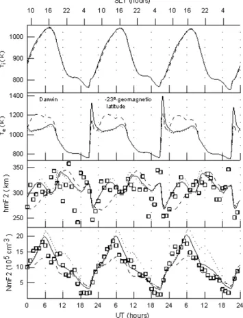
Fig. 3. Observed (squares) and calculated (lines) NmF2 and hmF2
(two lower panels), and electron and O+ion temperatures (two up-per panels) at the F2-region main peak altitude above the Darwin ionosonde station during 19–21 March 1988. SLT is the solar local time at the Darwin ionosonde station. The results obtained from the model of the ionosphere and plasmasphere using the SF E3, given
by dash-dotted line in Fig. 1, the NRLMSISE-00 neutral tempera-ture and densities, and the HWW90 wind as the input model param-eters are shown by dotted lines. Solid lines show the results given by the model with the corrected equatorial E3, given by the solid
line in Fig. 1, the corrected HWW90 wind, and the NRLMSISE-00 model with the corrected value of [O]. In the modification of the meridional wind in the Northern Hemisphere, the meridional HWW90 wind was decreased by 30 m sec−1between 10:14 UT and 13:44 UT and was increased by 30 m sec−1from 15:14 UT to 24:00 UT. The NRLMSISE-00 model [O] was increased by a factor of 1.5 in the 0–15◦geomagnetic latitude range of the North-ern Hemisphere from 05:14 UT to 09:44 UT. The results shown by dashed lines were calculated by the model with the same correc-tions of the NRLMSISE-00 [O] and meridional HWW90 wind as for the solid lines and when the value of the corrected E3, used in
producing results shown by the solid lines, was divided by a factor of 10 at all the studied geomagnetic latitudes.
in the equatorial E×B drift (see very large scattering in the measured vertical plasma drift in Figs. 1 and 2 of Scherliess and Fejer, 1999).
The equatorial daytime upward E×B drift resulting from E3lifts upward the ionospheric electrons and ions, and this
leads to the increase of hmF2 close to the geomagnetic
equa-tor. Ions and electrons then diffuse downward along the mag-netic field lines leading to the plasma “fountain”. The effect on NmF2 depends on the competition between the electron density reduction caused by the plasma outflow and the elec-tron density enhancement caused by the decrease in the loss rate of O+(4S) ions. Comparison between the results of cal-culations 1 and 3 or 1 and 4 shows that the increase in the equatorial daytime upward E×B drift leads to the decrease in NmF2, i.e. the NmF2 reduction caused by the plasma out-flow is stronger than the enhancement in NmF2 caused by the decrease in the loss rate of O+(4S) ions.
4.2 Comparison between the measured and modeled NmF2 and hmF2 in the geomagnetic meridian plane
The measured (squares) and calculated (lines) NmF2 and hmF2 are displayed in the two lower panels of Figs. 3-11 for 19-21 March 1988 above the Darwin (Fig. 3), Van-imo (Fig. 4), Manila (Fig. 5), Chung-Li (Fig. 6), Okinawa (Fig. 7), Yamagawa (Fig. 8), and Akita (Fig. 9) ionosonde stations, and above the MU radar (Fig. 10), while Te and Ti
at hmF2 above the sounders and the MU radar are presented in the two upper panels of these figures. Figure 11 shows the measured (squares) and calculated (lines) Ne(bottom panel),
Te(middle panel), and Ti (top panel) at the 400 km altitude
above the MU radar. The latitude and longitude location of the Kokubunji sounder is very close to that of the MU radar and the calculated hmF2, Ne, Te, and Ti above this
sounder are practically the same as those in Fig. 10. The model results using the combinations of the SF E3given by
dash-dotted line in Fig. 1, the NRLMSISE-00 neutral tem-perature and densities, and the HWW90 wind are shown by dotted lines. Solid lines show the results given by the model with the corrected equatorial E3 given by the solid line in
Fig. 1, the corrected NRLMSISE-00 [O] (the value of [O] was increased by a factor of 1.5 in the 0-15◦ geomagnetic latitude range of the Northern Hemisphere from 05:14 UT to 09:44 UT), and the corrected meridional neutral HWW90 wind. In the Northern Hemisphere, the meridional neutral wind, W, taken from the HWW90 wind model, was changed to W+1W , where 1W=-30 m/sec−1between 10:14 UT and 13:44 UT during 17–21 March 1988, 1W=30 m/sec−1from 15:14 UT to 24:00 UT and from 00:00 UT to 00:14 UT dur-ing 17–21 March 1988, 1W=20 m/sec−1from 01:14 UT to 06:14 UT on 21 March 1988, and 1W=0 from 00:14 UT to 09:14 UT during 17–21 March 1988 and from 07:14 UT to 09:14 UT on 21 March 1988. A linear interpolation between the values of 1W was used in the intermediate time peri-ods. This additional meridional neutral wind is used in the model calculations above the geomagnetic latitude of 24◦, while 1W=0 at the geomagnetic equator. A square interpo-lation of 1W is employed between 24◦and 0◦. Dashed lines were calculated by the model with the same corrections of the NRLMSISE-00 [O] and meridional neutral HWW90 wind as for solid lines and when the value of E3, used in producing
results shown by the solid lines, was divided by a factor of 10 at all the studied geomagnetic latitudes.
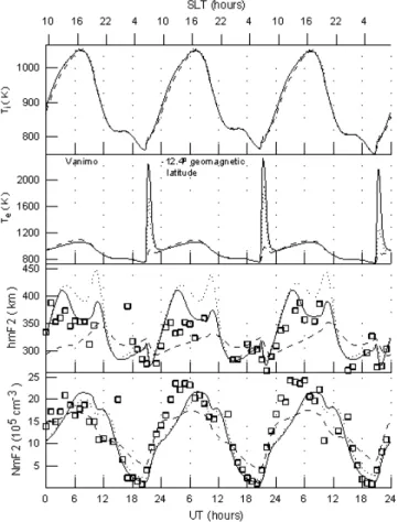
Fig. 4. From bottom to top, observed (squares) and calculated
(lines) of NmF2, hmF2, electron temperatures and O+ ion tem-peratures at the F2-region main peak altitude above the Vanimo ionosonde station during 19–21 March 1988. SLT is the solar lo-cal time at the Vanimo ionosonde station. The curves are the same as in Fig. 3.
By comparing dotted lines and squares in Figs. 4–6, it is seen that the calculated hmF2 is higher than the measured one from about 07:00 UT to about 11:00 UT on 19 March 1988 if the equatorial upward E×B drift given by Scher-liess and Fejer (1999) is employed. Use of the corrected equatorial E3 given by the solid line in Fig. 1 brings the
measured and modeled hmF2 into reasonable agreement, al-though there are some quantitative differences. On the other hand, it is well known (Su et al., 1997; Balan et al., 1998) that variations of hmF2 are controlled mainly by variations in the neutral wind and E3for low mid-latitudes, where the
MU radar and the Akita ionosonde station are located. How-ever, the HWW90 wind velocities are known to differ from observations (Oliver et al., 1990). For the present study the model HWW90 winds are modified, as explained above, to bring the modeled hmF2 in reasonable agreement with hmF2 measured by the MU radar and the Akita ionosonde station (see solid lines in Figs. 9–11).
We can expect that the neutral models have some inad-equacies in predicting the number densities with accuracy, and we have to change the number densities by correction
Fig. 5. From bottom to top, observed (squares) and calculated
(lines) of NmF2, hmF2, electron temperatures and O+ ion tem-peratures at the F2-region main peak altitude above the Manila ionosonde station during 19–21 March 1988. SLT is the solar lo-cal time at the Manila ionosonde station. The curves are the same as in Fig. 3.
factors at all altitudes to bring the modeled electron den-sities into agreement with the measurements. The value of [O] was increased by a factor of 1.5 in the 0–15◦ geo-magnetic latitude range of the Northern Hemisphere from 05:14 UT to 09:44 UT at all altitudes from the compari-son between the modeled NmF2 and NmF2 measured by the Manila ionosonde station. One can see from Fig. 5 that the NRLMSISE-00 model with the modified [O] improves the agreement with the measured NmF2 over the Manila ionosonde station.
The NRLMSISE-00 model can have some inadequacies in predicting the actual [N2] and [O2] with accuracy.
How-ever, to reach the same agreement between the measured and modeled NmF2 over the Manila ionosonde station, the val-ues of the NRLMSISE-00 [N2] and [O2] must be decreased
by a factor of 2 in the 0–15◦geomagnetic latitude range of the Northern Hemisphere from 05:14 UT to 09:44 UT at all altitudes without NRLMSISE-00 [O] corrections. Thus, the comparison between the NRLMSISE-00 [N2] and [O2]
de-crease and the NRLMSISE-00 [O] inde-crease does not show similarity and consistency in the magnitudes of their effects
Fig. 6. From bottom to top, observed (squares) and calculated
(lines) of NmF2, hmF2, electron temperatures and O+ ion tem-peratures at the F2-region main peak altitude above the Chung-Li ionosonde station during 19–21 March 1988. SLT is the solar local time at the Chung-Li ionosonde station. The curves are the same as in Fig. 3.
on NmF2 close to the geomagnetic equator. This difference in the reaction of the calculated NmF2 is large enough to pro-vide epro-vidence in favor of increasing [O] in comparison with reducing [N2] and [O2].
The middle-latitude daytime F2 peak electron density is proportional to [O]/[N2] (e.g. Rishbeth and Garriot, 1969).
In comparison with the middle-latitude ionosphere, the low-latitude ionosphere is special because of the constraints im-posed on electron and ion motions by the magnetic field and by the zonal component of the electric field. The model cal-culations of this work provide evidence that the dependence of NmF2 on [N2] and [O2] is weaker than the dependence
of NmF2 on [O] by day at low geomagnetic latitudes. We conclude that NmF2 is not proportional to [O]/[N2] or to
[O]/[O2] in the daytime ionosphere close to the geomagnetic
equator.
The comparison between the measured (squares) and mod-eled (lines) NmF2 and hmF2 latitude variations is shown in Fig. 12 at 08:00 UT (two upper panels) and 11:00 UT (two lower panels) on 19 March 1988. The combinations of the model input parameters used in the calculations of the model
Fig. 7. From bottom to top, observed (squares) and calculated
(lines) of NmF2, hmF2, electron temperatures and O+ ion tem-peratures at the F2-region main peak altitude above the Okinawa ionosonde station during 19–21 March 1988. SLT is the solar local time at the Okinawa ionosonde station. The curves are the same as in Fig. 3.
results shown by the solid and the dotted lines are the same as those for solid and dotted lines in Figs. 3–11, respectively. The comparison between the measured hmF2, NmF2 and the calculated results shown by dotted lines clearly indicates that there is the disagreement between the measured and modeled hmF2 and NmF2 at low geomagnetic latitudes at 08:00 UT and 11:00 UT on 19 March 1988 if the equatorial upward E×B drift given by Scherliess and Fejer (1999) is used. Fig-ure 12 shows that the modification of the equatorial upward E×B drift improves the agreement between the modeled and measured hmF2 and NmF2, and weakens the effect of the fountain in NmF2.
The model calculations produce the onset of the equato-rial anomaly crest formation close to 02:00 UT, in agree-ment with the ionosonde measureagree-ments. The model calcu-lations show that the crests disappear close to 15:00 UT. Fig-ures 3–9 show that the NmF2 values were not determined from ionograms at some ionosonde stations from 12:00 UT to 15:00 UT, and there is scattering in the data for this time period. As a result, the time of the crest disappearance is un-resolved from the measured NmF2. The principal feature of
Fig. 8. From bottom to top, observed (squares) and calculated
(lines) of NmF2, hmF2, electron temperatures and O+ ion tem-peratures at the F2-region main peak altitude above the Yamagawa ionosonde station during 19–21 March 1988. SLT is the solar local time at the Yamagawa ionosonde station. The curves are the same as in Fig. 3.
the equatorial anomaly is the crest-to-trough ratio. The mea-sured and modeled NmF2 show that the equatorial anomaly effect is most pronounced close to 06:00 UT.
Figure 13 presents the comparison between the measured (squares) and modeled (lines) NmF2 and hmF2 latitude vari-ations at 05:00 UT (two upper panels) and 06:00 UT (two lower panels) on 19 March 1988. The combinations of the model input parameters used in the calculations of the model results shown by the solid and dotted lines are the same as those for solid and dotted lines in Figs. 3–12, respectively. Dashed lines show the results produced by the model with the corrected equatorial E3given by the solid line in Fig. 1,
the NRLMSISE-00 neutral temperature and densities with the same correction of [O] as for the solid lines, and when the neutral wind is equal to zero.
The striking feature of the observed (squares) and mod-eled (solid and dotted lines) hmF2 and NmF2 is the ex-istence of an asymmetry in hmF2 and NmF2 between the northern and southern geomagnetic hemispheres. The crest electron density is greater in the northern geomagnetic hemi-sphere than that in the southern geomagnetic hemihemi-sphere,
Fig. 9. From bottom to top, observed (squares) and calculated
(lines) of NmF2, hmF2, electron temperatures and O+ion tempera-tures at the F2-region main peak altitude above the Akita ionosonde station during 19–21 March 1988. SLT is the local solar time at the Akita ionosonde station. The curves are the same as in Fig. 3.
while hmF2 of the crest electron density is less in the north-ern geomagnetic hemisphere than that in the southnorth-ern geo-magnetic hemisphere. It is clear that most of the asymmetry in hmF2 should come about through the asymmetry in the dynamical processes, which involve neutral winds and elec-tric fields. As can be seen from the comparison between the solid and dashed lines of Fig. 13, the asymmetry in hmF2 and NmF2 is sharply decreased if the model uses the zero neutral wind. We conclude that the neutral wind given by the HWW90 model of Hedin et al. (1991) is asymmetric about the geomagnetic equator, and this asymmetry deter-mines most of the asymmetry in hmF2 and NmF2 between the northern and southern geomagnetic hemispheres. This conclusion is in agreement with the previous results of Balan and Bailey (1995), Su et al. (1996), and Balan et al. (1997a, b). Dashed lines of Fig. 13 show that there is a small asym-metry in hmF2 and NmF2 between the northern and south-ern geomagnetic hemispheres for the zero neutral wind. This small asymmetry is caused by an asymmetry in the neutral temperature and densities between the northern and southern geomagnetic hemispheres.
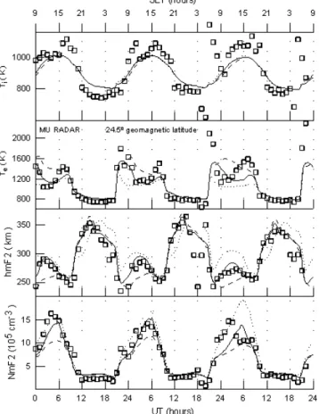
Fig. 10. Observed (squares) and calculated (lines) NmF2 and hmF2
(two lower panels), and electron and O+ion temperatures (two up-per panels) at the F2-region main peak altitude above the MU radar during 19–21 March 1988. SLT is the solar local time at the MU radar. The curves are the same as in Fig. 3.
To obtain a better understanding of the relative role of the E×B drift at low-latitudes, calculations have been carried out from the model when the value of E3, used in
produc-ing results shown by the solid lines, was divided by a factor of 10 at all the studied geomagnetic latitudes and when the corrections of the NRLMSISE-00 [O] and meridional neu-tral HWW90 wind are the same as for solid lines. The model results are shown by dashed lines in Figs. 3–11.
During most of the daytime period the E×B drift lifts the plasma from lower field lines to higher field lines, while dur-ing most of the night-time period this drift moves ions and electrons from higher field lines to lower field lines. Simul-taneously, the plasma diffuses along the magnetic field lines. The comparison between the solid and dashed lines in the bottom panel of Fig. 5 shows that, close to the geomagnetic equator, the NmF2 enhancement caused by the decrease in the plasma outflow is stronger than the reduction in NmF2 caused by the increase in the loss rate of O+(4S) ions. There-fore, the weakening of E3leads to the NmF2 increase by day
over the Manila sounder. The night-time NmF2 increase is a result of the daytime NmF2 increase and the decrease in the loss rate of O+(4S) ions due to the hmF2 increase caused by the weakening of E3over the Manila sounder. The complex
interplay of the physical processes described above for the
Fig. 11. The measured (squares) and calculated (lines) electron
den-sity (bottom panel) and electron (middle panel) and O+ion (top panel) temperatures at the 400 km altitude above the MU radar. The curves are the same as in Fig. 3.
Manila sounder determines the variations in NmF2 and hmF2 caused by the weakening of E3over the other sounders (see
Figs. 3–9).
The comparison between the solid and dashed lines in Figs. 10 and 11 shows that the E×B drift gives rise to con-siderable variations in NmF2 and hmF2, and in Neat 400 km
over the MU radar, and the magnitude of these daytime elec-tron density variations is less at hmF2 in comparison with that at 400 km. The weakening of E3 by a factor of 10
changes the simulated daytime NmF2 by a factor of 0.9–1.4, and the changes in hmF2 due to this weakening of E3are
be-tween -3 km and 34 km, while the maximum daytime change in Ne is a factor of 0.85–2.3 at 400 km. The change in the
night-time Neis less than that by day. The weakening of E3
by a factor of 10 produces the change in the calculated night-time NmF2 by a factor of 0.80–1.05 and the changes in hmF2 are between -10 km and 11 km by night, while the night-time change in Neis a factor of 0.86-1.05 at 400 km. It should be
noted that the studied changes in Ne are less pronounced at
higher altitudes in the topside ionosphere and plasmasphere above the MU radar. For example, the maximum electron density change caused by the weakening of E3 by a factor
of 10 is 19% and 2% at 1000 km above the MU radar by day and by night, respectively.
Fig. 12. Observed (squares) and calculated (lines) hmF2 and NmF2
at 08:00 UT (two upper panels) and 11:00 UT (two lower panels) on 19 March 1988. The measured hmF2 and NmF2 are taken from the ionospheric sounder station listed in Table 1. The curves are the same as in Fig. 3.
The model results presented in the bottom panels of Figs. 3–10 show that the magnitude of the electron density change caused by the weakening of E3by a factor of 10 is
decreased if the absolute value of the geomagnetic latitude is increased. As an example, above the Akita ionosonde sta-tion, this weakening in E3 changes the simulated daytime
NmF2 by a factor of 0.91–1.34 and hmF2 by the maximum value of 31 km, while the maximum daytime electron den-sity change is a factor of 0.90–1.96 at 400 km. We conclude that the use of the middle-latitude time dependent model of the ionosphere and plasmasphere, which does not take into account the E×B plasma drift, leads to noticeable errors in the calculated daytime electron density of the F2 region and a part of the topside ionosphere, even at geomagnetic latitudes of about 25◦-30◦.
It is found by Pavlov (2003) that the daytime magnitude of NmF2 should be reduced up to a maximum factor of 1.44 between -30◦ and +30◦of the geomagnetic latitude, due to enhanced vibrational excitation of N2and O2at high solar
activity during the geomagnetically quiet period of 7 Octo-ber 1957. We found that in the plane of the geomagnetic meridian at the geomagnetic longitude of 201◦the increase in the loss rate of O+(4S) ions, due to the vibrational excited N2and O2, leads to the maximum decrease in the calculated
NmF2 by a factor of 1.16 and to the maximum increase in
Fig. 13. Observed (squares) and calculated (lines) hmF2 and NmF2
at 08:00 UT (two upper panels) and 11:00 UT (two lower panels) on 19 March 1988. The measured hmF2 and NmF2 are taken from the ionospheric sounder station listed in Table 1. The solid and dotted curves are the same as in Fig. 3. Dashed lines show the results produced by the model with the corrected equatorial E3given by
the solid line in Fig. 1, zero neutral wind, and the NRLMSISE-00 neutral temperature and densities with the same correction of [O] as for the solid lines.
the calculated hmF2 of 5 km in the ionosphere between -30◦ and +30◦of the geomagnetic latitude at moderate solar activ-ity. We conclude that the effect of vibrationally excited N2
and O2on Neof the low-latitude ionosphere is decreased by
decreasing the solar activity level.
The measured hmF2 presented in Figs. 3–9 show large fluctuations. The possible source of this scatter in hmF2 is the dependence of hmF2 on M(3000)F2 and 1M given by Dudeney (1983), which determines hmF2 diurnal varia-tions with errors. The ionosondes listed in Table 1 are not located at the geomagnetic longitudes of 201◦, which is used
in the model calculations. This geomagnetic longitude dis-placement can explain a part of the disagreement between the modeled and measured hmF2 and NmF2 in Figs. 3–13. A part of these discrepancies is probably due to the uncer-tainties in the model inputs, such as the possible inability of the NRLMSIS-00 model to accurately predict the densities and temperature for the studied period at low-latitudes, and uncertainties in the neutral wind, EUV fluxes, chemical rate coefficients, photoionization, photoabsorption and electron impact cross sections for N2, O2, and O.
4.3 Electron and ion temperature variations
The two upper panels of Figs. 3–10 show the calculated (lines) and measured (squares) electron, Te, and ion, Ti,
tem-peratures at the F2-region main peak altitude for the 19–21 March 1988 time period above the Darwin (Fig. 3), Van-imo (Fig. 4), Manila (Fig. 5), Chung-Li (Fig. 6), Okinawa (Fig. 7), Yamagawa (Fig. 8), and Akita (Figu. 9) ionosonde stations and above the MU radar (Fig. 10). Figure 11 shows the measured (squares) and calculated (lines) electron (mid-dle panel) and O+ion (top panel) temperatures at the 400 km altitude above the MU radar.
It is evident from comparison between solid and dot-ted lines in Figs. 3–10 that the corrections in the equato-rial upward E×B drift, the model HWW90 wind, and the NRLMSISE-00 [O] produce negligible effects in Ti during
19–21 March 1988, while there are some electron tempera-ture variations due to these input model parameter changes after sunrise. The duration of the time period, where this dif-ference in the calculated electron temperatures is noticeable, is increased by increasing the absolute value of the geomag-netic latitude.
Figures 3–11 show that the diurnal variations of Te are
characterized by morning and evening peaks above the Dar-win, Yamagawa, Kokubunji, and Akita ionosonde stations and over the MU radar, while the model produces only morn-ing peaks and a broad daytime maximum in Te above the
Vanimo, Manila, Chung-Li, and Okinawa ionosonde sta-tions. The calculated evening Te peaks are less than those
measured by the MU radar. If we take into account the accuracy of the MU radar Te and Ti measurements (Sato
et al., 1989) and uncertainties of model calculations (see Sect. 4.2), then we conclude that Teand Ti observed by the
MU radar are in reasonable agreement with the model results shown by the solid lines in the two upper panels of Figs. 10– 11, although there are some quantitative differences. The rea-sonable agreement between the measured Teand Ti and the
modeled Teand Tidetermines the reliability of the calculated
Teand Ti at other geomagnetic latitudes.
The relative magnitudes of the cooling rates are of par-ticular interest for understanding the main processes, which determine the electron temperature. We found that the main cooling rates of thermal electrons in the low- and middle-latitude ionosphere are electron-ion Coulomb collisions, vi-brational excitation of N2and O2and rotational excitation of
N2.
The electron-ion cooling rate of thermal electrons, which is the predominant cooling rate at hmF2 and the main cooling rate in the plasmasphere and topside ionosphere, is propor-tional to Nesquared. As a result, variations in Necause
vari-ations in Te. It follows from the profiles of Te and Ti
mea-sured at Jicamarca that the enlargement of the altitude region with Te>Tioccurs at sunrise at all heights to at least 600 km
(McClure, 1969). Our calculations show that at sunrise, there is a rapid heating of the ambient electrons by photoelectrons, and the difference between the electron and neutral tempera-ture could be increased because nighttime electron densities
are less than those by day, and the electron cooling during morning conditions is less than that by day. This expands the altitude region at which Te>Ti near the equator and leads
to the sunrise electron temperature peaks at hmF2 altitudes above the ionosonde stations. After the abrupt increase at sunrise, the electron temperature decreases, owing to the in-creasing electron density due to the increase in the cooling rate of thermal electrons. An appearance, a magnitude, and a disappearance of a morning electron temperature peak at hmF2 depend on a minimum value of the night-time NmF2 before sunrise, because the morning NmF2 is a function of this minimum night-time NmF2.
Like the middle-latitude F-region ionosphere, the noc-turnal latitude F-region is maintained due to the low-latitude daytime F-region decay and by a downward flow of ionization from the plasmasphere. The role of a downward flow of ionization from the plasmasphere is increased before sunrise. A plasma tube length and total plasma tube con-tent are decreased with lowering the geomagnetic latitude. It means that an increase in the absolute value of the geo-magnetic latitude could lead to an increase in a downward flow of ionization from the plasmasphere, the increase in the night-time electron density before sunrise and the resulting decrease in the magnitude of the morning electron tempera-ture peak.
The downward night-time and morning E×B drift result-ing from E3<0 moves the ionospheric and plasmaspheric
electrons and ions from middle to low geomagnetic latitudes, and ions and electrons then diffuse downward along mag-netic field lines (the solid line in Fig. 1 shows that the require-ment of E3<0 is correct over the geomagnetic equator from
20:06 SLT to 24:00 SLT and from 24:00 SLT to 06:15 SLT, where SLT is the local solar time at the geomagnetic equa-tor and 201◦ geomagnetic longitude). The resulting effect of these physical processes on NmF2 depends on the com-petition between an enhancement in Necaused by a plasma
inflow and an decrease in Ne caused by an increase in the
loss rate of O+(4S) ions due to a NmF2 peak layer lowering. Figure 14 shows the calculated minimum night-time F2 layer peak electron density, NmF2min, (panel (a)) and its F2
peak altitude, hmF2min, (panel (b)), the dependence of the
calculated morning electron temperature peak, Tpeake , on the
geomagnetic latitude (panel (d)), and NmF2peak (panel (c)),
which is the value of NmF2 at the point of the morning elec-tron temperature peak calculation. The results shown by the solid lines in Fig. 14 were calculated by the model with the corrected equatorial E3given by the solid line in Fig. 1, the
corrected HWW90 wind, and the NRLMSISE-00 model with the corrected value of [O]. Dashed lines in Fig. 14 show the results given by the model with the same corrections of the NRLMSISE-00 [O] and meridional neutral HWW90 wind as for solid lines, but when the value of the corrected E3, used
in producing results shown by the solid lines, was divided by a factor of 10 at all the studied geomagnetic latitudes, only for the time periods when the equatorial value of E3,
equatorial E×B plasma drift is downward). Dotted lines in Fig. 14 show the results produced by the model with the cor-rected equatorial E3 given by the solid line in Fig. 1, zero
neutral wind, and the NRLMSISE-00 model with the same correction of [O] as for the solid lines.
By comparing the solid lines in the panels (a) and (c) of Fig. 14, it is seen that the geomagnetic latitude variation of NmF2peak is similar to the dependence of NmF2min on the
geomagnetic latitude. As a result, the model calculations of this work provide evidence that an appearance, a magni-tude, and a disappearance of a morning electron temperature peak at hmF2 depend on physical processes which determine NmF2min.
It follows from the comparison between the correspond-ing solid and dashed lines in Fig. 14 that the decrease in the equatorial night-time downward E×B drift by a factor of 10 leads to the increase in NmF2 between about -28◦ and
28◦geomagnetic latitudes, i.e. the NmF2 reduction caused
by the increase in the loss rate of O+(4S) ions is stronger than the enhancement in NmF2 caused by the plasma in-flow. The dashed lines in Fig. 14 show that the equatorial anomaly caused by the upward E×B drift by day is main-tained in the night-time low-latitude ionosphere due to the low-latitude daytime F-region decay, and a downward flow of ionization from the plasmasphere is not important. It fol-lows from Fig. 14 that the night-time and morning down-ward E×B drift causes the decrease of NmF2 and the re-sulting increase of the morning peak in Te. The night-time
and morning downward E×B drift becomes more effective in lowering Newith lowering the geomagnetic latitude., i.e.
a decrease in the absolute value of the geomagnetic latitude leads to the decrease in Ne close to sunrise, resulting in an
increase in the magnitude of the morning Te peak. It
fol-lows from panel (d) of Fig. 14 that the role of the night-time and morning downward E×B drift in creating the morning Tepeak is negligible above about 27◦and below about -27◦
geomagnetic latitude.
To obtain a better understanding of the relative role of the plasma drift caused by the neutral wind in the formation of the morning Tepeak, calculations have been carried out from
the model when the values of the components of the neu-tral wind, used in producing results shown by the solid lines, were taken to be zero and when the corrections in E3and the
NRLMSISE-00 [O] are the same as for solid lines. We com-pare the results of these model calculations (which are not shown in Figs. 3–10) with those shown by the solid lines in Figs. 3–10. We found that, above each ionosonde station of Table 1 and above the MU radar the magnitude of the morn-ing Tepeak produced by the model without the neutral wind
is increased by about 50–960 K and the width of the peak is decreased in comparison with the morning peak shown by the solid lines in Figs. 3–10.
By comparing the solid and dotted lines in the bottom panel of Fig. 14, it is seen that a wind, which is equator-ward by night in equinox at moderate solar activity, forces the F2 layer to lift upward to high altitudes of weak chemi-cal O+(4S) ion losses, increasing the electron density to high
Fig. 14. The calculated minimum night-time F2 layer peak electron
density, NmF2min, (panel (a)) and its F2 peak altitude, hmF2min
(panel (b)). The dependences of the calculated morning electron temperature peak, Tpeake , on the geomagnetic latitude is presented in
the panel (d). The panel (c) shows the calculated NmF2peak, which
is NmF2 at the point of the morning electron temperature peak cal-culation. Solid lines show the results given by the model with the corrected equatorial E3, given by the solid line in Fig. 1, the
rected HWW90 wind, and the NRLMSISE-00 model with the cor-rected value of [O]. Dotted lines show the results produced by the model with the corrected equatorial E3 given by the solid line in
Fig. 1, zero neutral wind, and the NRLMSISE-00 model with the same correction of [O] as for the solid lines. The results shown by dashed lines were calculated by the model with the same corrections of the NRLMSISE-00 [O] and meridional neutral HWW90 wind as for the solid lines, but only when the value of the corrected E3,
used in producing the results shown by the solid lines, divided by a factor of 10 at all the studied geomagnetic latitudes, only for the time periods when the equatorial value of E3, given by the solid
line in Fig. 1, is negative (i.e. when the equatorial E×B plasma drift is downward). The solid, dotted and dashed lines in panels (a, b) correspond to 04:41-05:29 SLT on 20 March, 05:09–05:28 SLT on 20 March, and 05:11–05:31 SLT on 20 March, respectively. The solid, dotted and dashed lines in panels (c, d) correspond to 05:48– 08:21 SLT on 20 March, 05:48–06:31 SLT on 20 March, and 06:33– 08:55 SLT on 20 March, respectively. Arrows at the top mark the locations of the Darwin, Vanimo, Manila, Chung-Li, Okinawa, Ya-magawa, Kokubunji, and Akita sounders at -23.0◦, -12.4◦, 3.4◦, 13.7◦, 15.4◦, 29.6◦, 20.5◦, 25.6◦, and 29.6◦geomagnetic latitudes, respectively.
Fig. 15. The latitude dependence of the daytime and evening
elec-tron temperature peaks (panel (d)), Tpeake , the time, SLTpeak, of the
electron temperature peak appearance (panel (c)), the value of the F2 peak layer density, NmF2peak, at SLTpeak(panel (a)), and the F2
peak layer altitude, hmF2peak(panel (b)) at SLTpeakon 19 March
1988. The electron temperature peak is taken to be closest to sun-set. The results shown by the solid lines were calculated by the model with the corrected zonal electric field, given by the solid line in Fig. 1, the corrected HWW90 wind, and the NRLMSISE-00 model with the corrected value of [O]. The dotted lines show the results produced by the model with the same zonal electric field as for the solid lines, zero neutral wind, and the NRLMSISE-00 model with the same correction of [O] as for the solid lines. The results shown by the dashed lines were calculated by the model with the same corrections of the NRLMSISE-00 [O] and meridional neutral HWW90 wind as for the solid lines, but only when the value of the corrected zonal electric field, used in producing results shown by the solid lines, was divided by a factor of 10 at all the studied geomag-netic latitudes. Arrows at the top mark the locations of the Darwin, Vanimo, Manila, Chung-Li, Okinawa, Yamagawa, Kokubunji, and Akita sounders at -23.0◦, -12.4◦, 3.4◦, 13.7◦, 15.4◦, 29.6◦, 20.5◦, 25.6◦, and 29.6◦geomagnetic latitudes, respectively.
values before sunrise. The increase in the absolute value of the geomagnetic latitude leads to the strengthening of the ef-fect of the plasma drift due to the neutral wind on the elec-tron density, the increase in the night-time elecelec-tron density before sunrise and the resulting decrease in the magnitude of the morning electron temperature peak. As it is seen from the comparison between the corresponding solid and dotted lines in the top panel of Fig. 14, the effect of the plasma drift
caused by the night-time neutral wind is to reduce the morn-ing Te peak through the increase in Ne at all geomagnetic
latitudes and the effect of this plasma drift on the formation of the morning Tepeak is decreased by decreasing the
abso-lute value of the geomagnetic latitude. It should be noted that a wind, which is poleward in the morning time periods de-creases hmF2, causing an increase in the loss rate of O+(4S) ions at hmF2, a decrease in NmF2 and helps to create an in-crease in Te, in agreement with the conclusions of Otsuka et
al. (1998).
Figure 15 shows the latitude dependence of the daytime and evening electron temperature peaks (panel (d)), Tpeake ,
the time, SLTpeak, of the electron temperature peak
appear-ance (panel (c)), the value of the F2 peak layer density, NmF2peak, at SLTpeak(panel (a)), and the F2 peak layer
al-titude, hmF2peak, at SLTpeak (panel (b)) on 19 March 1988.
The electron temperature peak is taken to be closest to sun-set. The results shown by the solid lines were calculated by the model with the corrected zonal electric field given by the solid line in Fig. 1, the corrected HWW90 wind, and the NRLMSISE-00 neutral temperature and densities with the corrected value of [O]. The dotted lines show the results pro-duced by the model with the same E3as for the solid lines,
zero neutral wind, and the NRLMSISE-00 neutral temper-ature and densities with the same correction of [O] as for the solid lines. The results shown by the dashed lines were calculated by the model with the same corrections of the NRLMSISE-00 [O] and meridional neutral HWW90 wind as for the solid lines, but only when the value of E3, used in
producing results shown by the solid lines, was divided by a factor of 10 at all the studied geomagnetic latitudes.
The present study has shown that the magnitude of the evening Tepeak and its time location are decreased by
lower-ing the geomagnetic latitude, and the evenlower-ing Tepeak
disap-pears from about -10◦to about 10◦geomagnetic latitude on
19 March, and only the afternoon daytime Tepeaks exist in
this latitude range if the corrected HWW90 wind (solid lines in Fig. 15) or zero wind (dashed lines in Fig. 15) are used in the calculations by the model with the corrected zonal electric field, given by crosses in Fig. 1, and the corrected NRLMSISE-00 atomic oxygen density.
It follows from the comparison between the solid and dot-ted lines in the panel (d) of Fig. 15 that the use of zero wind instead of the corrected HWW90 wind leads to a decrease in the magnitude of the evening electron temperature peak. The plasma drift along magnetic field lines due to the neutral wind can increase or decrease hmF2, leading to the decrease or increase in the loss rate of O+(4S) ions at hmF2, causing
an increase or a decrease in NmF2 and, as a result, leading to the disappearance or appearance of the evening peak in Te,
respectively.
A decrease in the production rate of O+ ions by solar ra-diation caused by a solar zenith angle increase results in a NmF2 decrease with time during an evening time period, and a feebly marked evening peak in Teis created by this evening
wind, which is poleward in equinox by day at moderate so-lar activity, forces the F2 layer to descend to low altitudes of heavy chemical O+(4S) ion losses, reducing N
eto low values
before sunset. Due to this poleward wind, the evening NmF2 decrease in time becomes strong, producing a strongly pro-nounced decrease in the thermal electron cooling rate and the resulting increase in the evening Tepeak, in agreement with
the results of Otsuka et al. (1998). The decrease in the abso-lute value of the geomagnetic latitude leads to the weakening of the effect of the plasma drift due to the neutral wind on Ne.
This explains the calculated latitude variations in the strength of the evening peak in Te.
The values of NmF2 and hmF2 which determine the mag-nitudes of the peaks in Teat hmF2 depend on the magnitude
and the direction of the E×B drift. By comparing the solid and dashed lines in Fig. 15, it can be seen that the weakening of E3by a factor of 10 causes the decrease in the magnitude
of the peak in Te between about -10◦and 10◦geomagnetic
latitude, and this magnitude is increased from about -10◦to -30◦ geomagnetic latitude and between about 10◦ and 30◦ geomagnetic latitude on 19 March. This weakening of E3
leads to the disappearance of an evening electron tempera-ture peak close to -21◦geomagnetic latitude and, as a result, only a daytime peak in Te exists on 19 March from about
-21◦to -30◦geomagnetic latitude (see the dashed line in the panel (c) of Fig. 15 and the dashed line in Fig. 3).
The comparison between the solid and dashed lines in Figs. 3–8 shows that the weakening of E3by a factor of 10
leads to the disappearance of the morning peak in Teover the
Manila sounder and to the decrease of the morning peak in Te
over the Yamagawa, Okinawa, Chung-Li, Manila, Vanimo, and Darwin sounders. It is also necessary to point out that the evening peak in Te is slightly less pronounced over the
Darwin and Yamagava ionosonde stations due to the weak-ening of E3by a factor of 10 (see Figs. 3 and 8). Figure 9
shows that this weakening of E3leads to the disappearance
of the evening Tepeak on 20–21 March 1988 over the Akita
sounder due to a decrease in the daytime NmF2 and an in-crease in the evening NmF2.
A comparison of the solid and dashed lines in the two up-per panels of Fig. 10 and in the middle and top panels of Fig. 11 shows the effect of the E×B drift on Te and Ti at
hmF2 (Fig. 10) and 400 km (Fig. 11) over the MU radar. It is seen that this very large decrease in the E×B drift can be important in changing the evening and morning Tepeaks by
eliminating the minimum between these peaks. The daytime decrease in Necaused by the weakening of E3by a factor of
10 leads to an increase in the daytime Tedue to the decrease
in the cooling rate of thermal electrons. The ion temperature depends on Te and Ne and, therefore, this weakening of E3
changes Ti. It should be noted that the increase in altitude
causes the increase of the relative role of the electron heat flow along the magnetic field line in comparison with cooling of thermal electrons, and the change in Te at 400 km is less
than that at hmF2. As a result, over the MU radar, the day-time Nedecrease leads to the daytime maximum increases in
Teof 400 K at hmF2 and 1000 K at 400 km, while the
maxi-mum night-time decrease in Tecaused by the increase in Ne
is close to 100 K at hmF2 and at 400 km. The changes in the daytime and night-time Ticaused by the weakening of E3by
a factor of 10 are less than 40 K at hmF2 and at 400 km over the MU radar. These model calculations provide evidence that the use of the middle-latitude time dependent model of the ionosphere and plasmasphere, which does not take into account the E×B plasma drift, leads to noticeable errors in the calculated daytime electron temperature of the F2 region and a part of the topside ionosphere, even at geomagnetic latitudes of about 25◦-30◦.
5 Conclusions
We have presented a comparison between the modeled NmF2 and hmF2, and NmF2 and hmF2, which were observed by the Akita, Kokubunji, Yamagawa, Okinawa, Chung-Li, Manila, Vanimo, and Darwin ionospheric sounders and by the MU radar during 19–21 March 1988. A comparison between the calculated Te and Ti and those measured by the MU radar
is presented for 19–21 March 1988. The model reproduces major features of the data.
It is found that there is a large disagreement between the measured and modeled hmF2 from about 07:00 UT to about 11:00 UT if the equatorial upward E×B drift given by Scherliess and Fejer (1999) is used. The discovered mod-ification of the equatorial upward E×B drift weakens the effect of the fountain in NmF2, bringing the modeled and measured hmF2 and NmF2 into reasonable agreement. In agreement with the ionosonde measurements of NmF2, the model produces the onset of the equatorial anomaly crest for-mation close to 02:00 UT, shows that the equatorial anomaly effect is most pronounced close to 06:00 UT, and produces the crest disappearance close to 15:00 UT. It has been found that the north-south asymmetries in the observed NmF2 and hmF2 about the geomagnetic equator are mainly caused by the asymmetry in the neutral wind about the geomagnetic equator due to the displacement of the geographic and mag-netic equators and the magmag-netic declination angle.
It is shown that the dependence of NmF2 on [N2] and [O2]
is weaker than the dependence of NmF2 on [O] by day close to the geomagnetic equator. We conclude that NmF2 is not proportional to [O]/[N2] or to [O]/[O2] in the daytime
iono-sphere close to the geomagnetic equator. It is shown that the increase in the loss rate of O+(4S) ions, due to the vibrational excited N2 and O2, leads to the decrease in the calculated
NmF2, up to a maximum factor of 1.16 and to the increase in the calculated hmF2, up to a maximum value of 5 km be-tween -30◦and +30◦geomagnetic latitude at moderate solar
activity.
The diurnal variations of Te are characterized by
morn-ing and evenmorn-ing peaks above the Yamagawa, Kokubunji, and Akita ionosonde stations and over the MU radar, while there is only a morning peak in Te above the Darwin, Vanimo,
Manila, Chung-Li, and Okinawa ionosonde stations. There is a rapid heating of daytime electrons by photoelectrons, and