HAL Id: hal-00317080
https://hal.archives-ouvertes.fr/hal-00317080
Submitted on 1 Jan 2002
HAL is a multi-disciplinary open access
archive for the deposit and dissemination of
sci-entific research documents, whether they are
pub-lished or not. The documents may come from
teaching and research institutions in France or
abroad, or from public or private research centers.
L’archive ouverte pluridisciplinaire HAL, est
destinée au dépôt et à la diffusion de documents
scientifiques de niveau recherche, publiés ou non,
émanant des établissements d’enseignement et de
recherche français ou étrangers, des laboratoires
publics ou privés.
Comparisons of high latitude E > 20 MeV proton
geomagnetic cutoff observations with predictions of the
SEPTR model
S. Kahler, A. Ling
To cite this version:
S. Kahler, A. Ling. Comparisons of high latitude E > 20 MeV proton geomagnetic cutoff observations
with predictions of the SEPTR model. Annales Geophysicae, European Geosciences Union, 2002, 20
(7), pp.997-1005. �hal-00317080�
Geophysicae
Comparisons of high latitude E > 20 MeV proton geomagnetic
cutoff observations with predictions of the SEPTR model
S. Kahler1and A. Ling2
1Air Force Research Laboratory, Space Vehicles Directorate, Hanscom Air Force Base, Massachusetts 01731, USA 2Radex Corporation, 3 Preston Court, Bedford, Massachusetts 01730, USA
Received: 9 October 2001 – Revised: 8 March 2002 – Accepted: 11 March 2002
Abstract. Radiation effects from solar energetic proton (SEP) events are a concern when the International Space Station reaches high latitudes accessible to SEPs. We use data from the 20–29 and 29–64 MeV proton channels of the Proton/Electron Telescope on the SAMPEX satellite during nine large SEP events to determine the experimental geo-graphic cutoff latitudes for the two energy ranges. These are compared with calculated cutoff latitudes based on a com-puter model, SEPTR (solar energetic particle tracer). The observed cutoff latitudes are systematically equatorward of the latitudes calculated by the SEPTR program using a Tsy-ganenko field model, but that model produces mean values of ∼2◦ for latitudinal differences with observations, 1Lat, which are ∼3 times smaller than those using the 1995 In-ternational Geomagnetic Reference Field model alone. The number distributions of 1Lat are peaked near 0◦and decline toward higher values. With the Tsyganenko model, we find no significant trend in either the 1Lat or their variances with increasing Kp.
Key words. Interplanetary physics (energetic particles) –
Magnetospheric physics (polar cap phenomena) – Space plasma physics (charged particle motion and acceleration)
1 Introduction
1.1 Radiation and the International Space Station
Space radiation is now recognized as a serious hazard for satellite operations, communications, and human space flights (White and Averner, 2001). With the construction of the International Space Station (ISS), the vulnerability of the human crews on the ISS to the effects of solar ener-getic proton (SEP) events has become an important concern (Turner, 2001). A recent report by the U.S. National Re-search Council (Siscoe et al., 2000) focused on radiation risk Correspondence to: S. Kahler
(stephen.kahler@hanscom.af.mil)
management during the ISS construction and concluded that the probability of a significant high-latitude SEP event during an ISS construction flight is nearly unity. The report recom-mended the development of models to specify the intensity of SEPs and the geographical zones accessible to them. In particular, it urged the development of methods to map lati-tudinal cutoffs for SEPs at the altitudes of the ISS. Another recommendation was to extend the range of SEP predictions from the present ≥10 MeV range to several steps in the bio-logically effective energy range of 10 to 100 MeV.
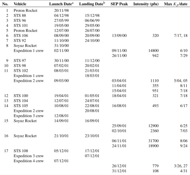
The ISS orbit was originally planned for a low-altitude, low-inclination orbit of 28.5◦, but with the 1993 agreement to include Russian launch capabilities in the ISS program, it was necessary to increase the orbital inclination to 51.6◦to the equator, placing parts of its orbit in high-latitude regions accessible to SEPs. In addition, the construction schedule was roughly in phase with the solar activity cycle, suggesting an enhanced probability of exposure of astronauts to SEPs. Table 1 compares the chronology of the ISS flights with the occurrence of large SEP events listed by the NOAA Space Environment Center at the web addresshttp://umbra. nascom.nasa.gov/SEP/seps.html. Proton intensi-ties are integral 5-min averages for energies E > 10 MeV, given in particle flux units (pfu), where 1 pfu = 1 p cm−2sr−1 s−1, measured by GOES spacecraft at geosynchronous or-bit. We give the peak dates of the largest (> 100 pfu) SEP events since the first flight of the ISS construction program in November 1998.
At the time of writing, 17 of the ≥ 40 flights on the NASA manifest for the ISS construction have occurred. One recent flight, the STS-100, from 19 April to 1 May 2001, occurred just after two intense SEP events on 15 and 18 April, al-though the intensity had fallen to < 20 pfu at the time of the launch and continued to decline during the mission. How-ever, a significant earlier SEP event occurred with a peak in the middle of the STS 106 mission in September 2000. A six-hour extravehicular activity (EVA) on STS 106 took place on 11 September , one day before the SEP event onset. These events have already confirmed the prediction (Siscoe
998 S. Kahler and A. Ling: Comparisons of high latitude E > 20 MeV proton geomagnetic cutoff observations
Table 1. ISS flights and SEP events
No. Vehicle Launch Datea Landing Dateb SEP Peak Intensity (pfu) Max Kp/date
1 Proton Rocket 20/11/98 2 STS 88 04/12/98 15/12/98 3 STS 96 27/05/99 06/06/99 4 STS 101 19/05/00 29/05/00 5 Proton Rocket 12/07/00 26/07/00 6 STS 106 08/09/00 20/09/00 13/09/00 320 7/17, 18 7 STS 92 11/10/00 24/10/00 8 Soyuz Rocket 31/10/00 Expedition 1 crew 02/11/00 09/11/00 14800 6/10 26/11/00 942 7/29 9 STS 97 30/11/00 11/12/00 10 STS 98 07/02/01 20/02/01 11 STS 102 08/03/01 21/03/01 Expedition 1 crew 18/03/01 Expedition 2 crew 09/03/00 03/04/01 1110 5/04, 05 11/04/01 355 8/11 15/04/01 951 7/18 12 STS 100 19/04/01 01/05/01 18/04/01 321 7/18 13 STS 104 12/07/01 24/07/01 14 STS 105 10/08/01 22/08/01 16/08/01 493 6/17 Expedition 2 crew 20/08/01 Expedition 3 crew 12/08/01 15 Soyuz Rocket 14/09/01 16/09/01 25/09/01 12900 6/25 02/10/01 2360 7/03 16 Soyuz Rocket 21/10/01 23/10/01 06/11/01 31700 8/06 24/11/01 18900 9/24 17 STS 108 05/12/01 17/12/01 Expedition 3 crew 07/12/01 Expedition 4 crew 07/12/01 26/12/01 779 3/26, 27 31/12/01 108 4/31
a ISS occupation start dates for crews
b ISS occupation end dates for crews or rocket docking dates
et al., 2000) that at least two of the planned ISS construction flights would overlap a significant SEP event. Even after the completion of the construction phase, one or two EVAs per month are expected to occur over the life of the ISS. Note that the ISS has been occupied by human crews continuously since November 2000.
The ISS radiation problem is compounded by the statisti-cal tendency for fast CME-driven shocks associated with the SEP events also to produce periods of enhanced geomagnetic activity (Shea et al., 1999) when they impact the Earth. The resulting polar impact zones of SEPs tend to increase with in-creasing SEP intensities (Shea et al., 1999), especially when
E >10 MeV intensities exceed 100 pfu. In Table 1 we show the peak value of Kp, the planetary index of geomagnetic ac-tivity, which occurred during the times of the SEP events. Kp values range from 0, the least disturbed, to 9, the most dis-turbed, with 3 ≤ Kp ≤ 5 considered moderately disturbed.
Most peak Kpvalues of the SEP events of Table 1 are in the very disturbed (Kp ≥ 6) range, which occurred only 2% of the time during solar cycle 22 (Shea et al., 1999).
1.2 SEP geomagnetic cutoff models
The problem of calculating trajectories of charged particles in the geomagnetic field was first modeled with dipole mag-netic fields in the 1930s by St¨ormer (1955). The basic par-ticle parameter is the rigidity R, defined as the parpar-ticle mo-mentum divided by its charge. An important parameter of the calculations is the cutoff rigidity Rcutoff, the minimum mag-netic rigidity of a charged particle that can reach a given point in space from infinity with a given direction of arrival. See re-views by Hoffman and Sauer (1968) and Smart et al. (2000) for early and very recent efforts, respectively, to determine
Rcutoff for the geomagnetic field. Rcutoff is calculated for a given point in space by integrating the equations of
mo-tion for an oppositely charged particle moving away from the point in space. The trajectory of an approaching pro-ton is, therefore, calculated in reverse, and the calculation is done for protons over a range of rigidities. Each trajec-tory either goes to infinity or some specified distance from the Earth, collides with the Earth, or spends an indetermi-nately long time trapped in the model geomagnetic field. The first group of trajectories are those of the allowed rigidities (R > Rcutoff), and those of the latter two are the forbidden rigidities. The presence of trajectories which collide with the solid Earth provides a complication by producing a penum-bra of bands of alternating allowed and forbidden rigidities above Rcutoff, with RL as the lower cutoff rigidity below which all rigidities are forbidden, and RU as the upper cutoff rigidity above which all rigidities are allowed (e.g. Smart et al., 2000). An effective cutoff rigidity in a given direction,
RC, is determined by either linear averaging of the allowed bands in the penumbra (Shea et al., 1965) or by functions weighted for the particle spectrum and/or detector response (Cooke et al., 1991).
A proton detector at a point in space will have a finite view angle, so the range of directions from which protons can arrive in the detector must also be considered in deter-mining the detector cutoff rigidity. Since this can result in a very computer-intensive effort to calculate trajectories for a range of proton rigidities, each over a range of incident angles, for each point in space, trajectories of only limited sets of zenith angles or planes at specific points in geospace have been calculated (Schwartz, 1959; Cooke et al., 1991). Cutoff rigidities are highest in the eastern and lowest in the western directions, but the penumbral structures vary consid-erably with change in incident angle. Recent work of Clem et al. (1997) has compared the vertical effective cutoff rigid-ity, RC, with an apparent cutoff rigidity, determined by an appropriate averaging over calculated values of RC extend-ing to 60◦off the vertical axis. Working in the 2 to 13 GV range, they found that apparent rigidities generally exceeded vertical RCby 0.1 to 0.6 GV. If this result holds in the rigid-ity range of our interest (0.2 to 0.3 GV), then values of RC based only on vertical cutoff calculations are underestimates of apparent cutoff rigidities.
The geomagnetic field model is a primary factor in the cal-culation of RC. The majority of proton magnetospheric tra-jectory calculations use the International Geomagnetic Ref-erence Field (IGRF) (Langel et al., 1991), which represents the main geomagnetic field, combined with a model of mag-netospheric current systems (Fl¨uckiger et al., 1991; Boberg et al., 1995; Tsyganenko, 2001). The preferred example of the latter model is that of Tsyganenko (1989; hereafter TSYG89), which includes currents during times of low to moderate (Kp ≤5) geomagnetic disturbances and takes Kp as an input parameter. This system was extended to large ge-omagnetic disturbances by Boberg et al. (1995). The result of including these current systems reduces the calculated RC, particularly at high geomagnetic latitudes.
Recent calculations of RC for vertically incident protons mapped on to a world grid (Smart et al., 2000) have been
car-ried out with a 1990 epoch Definitive IGRF (DGRF90) (Lan-gel, 1992) for altitudes of 20 km (Smart and Shea, 1997a) and 450 km (Smart and Shea, 1997b). The latter calcula-tion, chosen for its application to the ISS, was updated for a 1995 epoch IGRF (Sabaka et al., 1997) and TSYG89 for quiet (Kp = 0 and 2) and disturbed (Kp = 5 and 5 with a ring current model equivalent of Dst index of −300) geo-magnetic conditions by Smart et al. (1999a) and (1999b), re-spectively. The significant reductions in RC at 450 km with increasing geomagnetic activity, extended to Dst = −500, were illustrated by Smart et al. (1999c). Since RC at any geographical location is dependent on local time, all these calculations were averaged for local times of 00:00, 06:00, 12:00, and 18:00 UT.
1.3 Experimental observations of geomagnetic cutoffs While a particle detector on a satellite with a high-latitude orbit can survey the cutoff latitudes for its particular particle rigidity range, there are several limiting factors to be consid-ered in using such data sets to test computed cutoff models. First, protons in the 10 < E < 100 MeV range, which is of primary consideration for the ISS (Siscoe et al., 2000), will be enhanced above the background only during times of SEP events. Second, time-intensity profiles from detec-tors with broad bands of energy response may not show the sharp drops needed for precise determinations of cutoff lat-itudes. More important, while cutoff calculations are typi-cally done only for vertical cutoffs (e.g. Smart et al., 1999a, b), the finite detector geometries allow for particles from a range of directions to be counted. Since the cutoffs at a given point vary significantly with azimuthal angle (e.g. Clem et al., 1997), the calculated vertical cutoff latitudes may not cor-respond well to observed cutoff latitudes. A notable excep-tion was the cosmic ray experiment on the HEAO-3 satellite that recorded the energy, charge, and direction of every inci-dent cosmic ray ion. Comparison of those HEAO-3 data with the cutoff predictions verified the principal features of the predictions, but showed that the predicted cutoffs were about 5% higher than those observed (Smart and Shea, 1994). This result was consistent with earlier comparisons, as briefly re-viewed by Ogliore et al. (2001). This means that for a given particle rigidity, the observed geomagnetic cutoffs lie equa-torward of the calculated values.
Near real-time color-coded displays of global distributions of energetic particle counting rates from the polar-orbiting NOAA POES satellites are currently available at the web site http://www.sec.noaa.gov/tiger/. Proton counts from omnidi-rectional detectors with four energy channels in the range 16–275 MeV are shown plotted on world grids, with E > 15 MeV proton counts displayed on geographic polar plots. While not suitable for the measurement of geomagnetic cut-offs RCwe seek here, they allow for a comprehensive view of the zones of SEP precipitation in significant SEP events.
The optimal instruments for determining geomagnetic cut-offs have been the Mass Spectrometer Telescope (MAST) and Proton/Electron Telescope (PET) on the Solar,
Anoma-1000 S. Kahler and A. Ling: Comparisons of high latitude E > 20 MeV proton geomagnetic cutoff observations
Fig. 1. The world grid for 3 November 1992 showing the observed PET 20–29 MeV proton cutoffs (crosses), the calculated SEPTR
Tsy-ganenko field cutoffs (open circles), and the calculated SEPTR IGRF field cutoffs (solid circles). High-latitude and SAA portions of the SAMPEX orbit are shown. In general, the IGRF cutoffs are poleward of the Tsyganenko cutoffs and further poleward of the PET cutoffs.
lous, and Magnetospheric Particle Explorer (SAMPEX) spacecraft, which was launched into a 520 km × 670 km 82◦ inclination orbit in 1992 (Ogliore et al., 2001). In normal operations the MAST and PET instruments are zenith point-ing (Leske et al., 2001), so that vertical geomagnetic cutoffs can be determined on each side of each polar passage, or four times per orbit. Recently, Ogliore et al. (2001) deter-mined RC for cosmic ray nuclei from MAST in the rigidity range 500 < R < 1700 MV. Their particle selection crite-ria discriminated against SEPs, anomalous cosmic rays, and geomagnetically disturbed times. They plotted their cutoffs as functions of invariant latitude, 3, defined as the magnetic latitude at which a given ideal dipole field line intersects the Earth’s surface, and is related to the McIlwain L parameter by L = cos−2(3) (Hoffman and Sauer, 1968; Smart and Shea, 1994). In this coordinate system
RC = ×L−2GV = C × cos4(3)GV , (1) where C is a constant, and the blocking effects of the solid Earth are ignored. Ogliore et al. (2001) found a best fit for their cutoffs to be RC=15.062×cos4(3)−0.363 GV, lower than that predicted by the relation RC=14.5 × cos4(3)GV, which was recommended for vertical cutoffs by Smart and Shea (1994) using the DGRF90. This result means that at high latitudes (3 > 50◦), a given RC lies several degrees equatorward of the Smart and Shea (1994) calculation.
The SAMPEX PET instrument measures protons in the 20–29 MeV and 29–64 MeV energy ranges with a full-width opening angle of 58◦(Cook et al., 1993). PET observations were used to determine invariant cutoff latitudes with which SEP ionic charge states could be determined from other SAMPEX instruments (e.g. Oetliker et al., 1997; Mazur et al., 1999). Recently, Leske et al. (2001) have examined PET proton and MAST 8–15 MeV/nucleon He observations to de-termine the invariant cutoff latitudes, using the DGRF90, for six large SEP events from 1992 to 1998. They found that the cutoff latitudes correlated with the geomagnetic activity parameters Kp and Dst, although the correlation could be poor at certain times, such as the onset of a geomagnetic storm. At a given value of Kp or Dst the spread in cut-off latitudes was ∼2◦−3◦. Correcting for Dst effects, they found an invariant cutoff latitude of ∼64◦for MAST obser-vations at ∼300 MV. The above Eq. (1) suggested by Smart and Shea (1994), yields an invariant cutoff latitude of 67.7◦ for RC =300 MV, again several degrees poleward from the observed value.
1.4 The SEPTR programme
The Solar Energetic Particle Tracer (SEPTR) model is based on a Ph.D. thesis of Orloff (1998). SEPTR (Freeman and Orloff, 2001) takes a number of variable input parameters and uses several modifications to the basic particle trajectory
Table 2. Average latitudinal differences 1Lat for the Tsyganenko field in the nine analyzed SEP events
Data Interval Max Kp 1Lat 20–29 MeV 1Lat 29–64 MeV
30/10–06/11/92 6 2.7◦±1.6◦ 1.6◦±1.3◦ 06/11–10/11/97 7 3.0◦±2.5◦ 2.2◦±2.1◦ 25/08–29/08/98 8 2.6◦±2.5◦ 1.8◦±1.8◦ 30/09–02/10/98 5+ 2.4◦±2.2◦ 2.1◦±1.9◦ 12/09–16/09/00 6+ 2.5◦±1.8◦ 1.7◦±1.6◦ 09/11–15/11/00 6+ 1.8◦±1.3◦ 1.6◦±1.4◦ 24/11–29/11/00 7− 2.9◦±1.6◦ 2.0◦±1.4◦ 30/03–31/03/01 9− 3.5◦±3.1◦ 1.9◦±2.1◦ 03/04–19/04/01 8+ 2.2◦±1.7◦ 1.7◦±1.3◦ Average of all events: 2.5◦±1.9◦ 1.8◦±1.5◦
Fig. 2. Top panels: Histograms of numbers of cases of 1Lat for the
20–29 MeV protons with the IGRF model (top) and Tsyganenko model (bottom). The observing period is 25 to 29 August 1998. Each case is a difference between the calculated (IGRF or Tsy-ganenko) and observed PET geographic cutoff latitudes. Bottom panel: Same as the above but for the 29–64 MeV protons.
Fig. 3. Top panels: Histograms of numbers of cases for all nine SEP
events of 1Lat for the 20–29 MeV protons with the IGRF model (top) and Tsyganenko model (bottom). Each case is a difference between the calculated (IGRF or Tsyganenko) and observed PET geographic cutoff latitudes. Bottom panel: Same as the above but for the 29–64 MeV protons.
1002 S. Kahler and A. Ling: Comparisons of high latitude E > 20 MeV proton geomagnetic cutoff observations
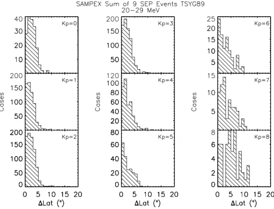
Fig. 4. Histograms of numbers of cases of 1Lat for 20–29 MeV protons and the Tsyganenko model binned by Kp.
calculation described by Smart et al. (2000) to calculate val-ues of RC at a given location. The model has been validated by several consistency checks and by comparisons of calcu-lated world grids of RCwith those of Smart and Shea (1985) using the same input geomagnetic field models (Freeman and Orloff, 2001).
Although SEPTR was designed to calculate RCat a spe-cific location, we will use SEPTR to determine whether ver-tically incident particles of a given rigidity R can reach a given point in space. For the SEPTR input values we use the positions of the SAMPEX spacecraft along its orbit and the rigidities of 0.215 GV and 0.298 GV, corresponding to the mean energies of the 20–29 MeV and 29–64 MeV pro-ton channels of the PET. The trajectories from each point are calculated until: (1) the proton reaches 25 RE; (2) the proton trajectory intercepts the solid Earth; (3) the particle travels a distance of 500 RE; or (4) the time of proton propa-gation reaches 1000 time units, where the SEPTR time unit is 0.0212 s. Only trajectories satisfying condition (1) are con-sidered to be allowed. We will use as input field models the 1995 IGRF (Sabaka et al., 1997) and the TSYG89, which is valid for Kp ≤ 5. When Kp > 5, we use the TSYG89 with Kp =5. We do not use here the Boberg et al. (1995) modification to the TSYG89 for Kp>5.
2 Data analysis
We selected for analysis nine SEP events with high E > 20 MeV intensities and at least moderate peak values of Kp.
Table 2 gives the selected dates of analysis and the maximum
Kpduring each period. The first four events were also ana-lyzed by Leske et al. (2001). For each event we determined the geographical cutoff locations for the 20–29 MeV and 29– 64 MeV protons of the PET detector. Each cutoff location was taken to be the point at which the rate of change of the PET SEP intensities, measured with 6-second time resolu-tion, was maximum. For each full day of data there were 15 or 16 orbits, so with two cutoff points for each polar pass there were up to 64 cutoff locations per day. All cutoff loca-tions were tabulated and plotted on a world grid for each day, as shown in Fig. 1.
Along each SAMPEX orbit the geographic cutoff loca-tions were calculated with SEPTR for assumed PET pro-ton rigidities of 0.215 and 0.298 GV and a fixed altitude of 600 km, using first the 1995 IGRF (Sabaka et al., 1997) and then the combined 1995 IGRF and TSYG89 reference field. We refer to these fields simply as the IGRF and TSYG89 fields, respectively. The calculated cutoff locations for the two fields were also plotted on the world grids. We found that the calculated cutoff latitudes are almost always poleward of the observed cutoff latitudes, as the example of Fig. 1 shows. For each orbit we compared the calculated cutoff latitudes of each field model with the observed cutoff latitudes for each PET energy range. For each SEP event we compiled the histograms of numbers of cases versus 1Lat, the differ-ence between the calculated and observed geographic cutoff latitudes, and calculated their mean values and variances. In Fig. 2 we show the distributions for the August 1998 SEP
event. We note first that the IGRF model provides a much worse fit than does the TSYG89 model, by a factor of ∼3, for both energy bands. Second, the values of 1Lat are larger for the 20–29 MeV protons than for the 29–64 MeV protons. Third, the distributions are very different for the two models. The IGRF values are peaked near their mean values, while the TSYG89 values are peaked near 0◦and decline with in-creasing 1Lat. The high variances of the latter values are due to the small number of cases of large 1Lat. These prop-erties of the August 1998 event are characteristic of all nine SEP events. In the last two columns of Table 2 we show the means and variances for the TSYG89 model. The bottom row of the table gives the result of summing over all the event orbits, and the histograms are shown in Fig. 3.
We have also compiled histograms of 1Lat as a function of Kp and shown them for the 20–29 MeV protons and the TSYG89 model in Fig. 4. In all of the cases, except where
Kp ≥ 7, the distributions are peaked within 2◦ of 0◦ and have the same basic shapes as those of the TSYG89 model of Fig. 3. Figure 5 compares the values of 1Lat as a function of
Kpfor the IGRF and TSYG89 models. It is not surprising to find that the TSYG89 model is superior to the IGRF model, but we find that the TSYG89 model is nearly independent of
Kp. There is a small but insignificant increase in 1Lat for
Kp ≥ 6, above the range for which the TSYG89 model is valid.
Several possible sources of error could contribute to the variances shown in Fig. 5. We pointed out in Sect. 1 that
Rcutoff at any location is not sharp but rather is character-ized by a penumbra over which RCmust be defined. Thus, the imprecise value of RCmight be a source of the variance. However, we have used SEPTR only to calculate whether an interplanetary 0.215 GV or 0.298 GV proton has access to a particular point in the SAMPEX orbit. Since we have very rarely found a SAMPEX polar-cap orbital boundary charac-terized by any fluctuation in the step function between al-lowed and forbidden regions, calculated at 6-second inter-vals, we do not consider this to be a source of the variance.
Another contribution to the variances could be our approx-imation to the energy ranges of the PET detectors by taking the mean energies, rather than weighting them with an sumed power-law rigidity or energy distribution. If we as-sume a differential power law in energy E with an exponent
γ = −3, then the mean energies in the two PET channels are 23.3 MeV and 37.4 MeV. These lower mean energies would result in higher, more poleward calculated cutoff latitudes and would increase the values of 1Lat in Table 2. We can use Eq. (1) with C = 14.5 to approximate these increases in ge-ographical latitudes L by calculating the changes in invariant latitudes 3 resulting from the corresponding lower values of
RC. For the 20–29 MeV protons 3 increases from 69.55◦to 69.68◦, an increase of 0.13◦and only a small fraction of the average 1Lat = 2.5◦shown in Table 2. For the 29–46 MeV protons, however, 3 increases from 67.71◦to 68.32◦, an in-crease of 0.6◦and a large fraction of the average of 1Lat = 1.8◦in Table 2. The resulting increase to 1Lat = 2.4◦would make it comparable to that of the 20–29 MeV proton value.
Fig. 5. Top: Comparison of average values of 1Lat for 20–29 MeV
protons and for the IGRF model and the Tsyganenko model binned by Kp. Bottom: Same as top except for 29–64 MeV protons.
Cutoff variations with local time may be a minor contri-bution to the values of 1Lat, but they tend to produce small offsets from the circles of constant 3, as discussed by Leske et al. (2001). The TSYG89 model that we used incorporates the variations of local time, so they should not be a signifi-cant factor in the variances.
Another source of the variances may be the approxima-tion we have made to compare the observed and calculated geographic cutoff latitudes as though they coincided in lon-gitude, when in fact, they lie at different longitudes along the SAMPEX orbit. If contours of constant RC are inclined to circles of geographic latitude, and the SAMPEX orbit is nearly tangent to those contours, the calculated 1Lat could be larger than that at a fixed longitude. We can estimate the error from this effect by assuming that the geomagnetic dipole is tilted about 11◦ to the rotational axis, so that the geographic longitudinal gradient of a given 3 should be ≤ 22◦/180◦, or ≤ 0.12◦per degree of longitude. From Fig. 1 we estimate that the geographical longitudinal differences between the observed and calculated cutoffs for a given orbit are ≤ 5◦, so the effective error for a given 1Lat is ≤ 0.6◦.
1004 S. Kahler and A. Ling: Comparisons of high latitude E > 20 MeV proton geomagnetic cutoff observations Note that this effect approaches 0◦ when the cutoffs lie in
the regions of lowest geographic latitudes most important for the ISS. From the symmetry of the orbits we see that the net effect could be negative or positive and hence will increase the widths of the distributions of 1Lat, but not change the resulting average values of 1Lat.
3 Discussion
We have compared the calculated geomagnetic cutoff lati-tudes of the SEPTR program with the 20–29 and 29–64 MeV proton cutoff latitudes observed with the SAMPEX PET de-tector for nine SEP events. The TSYG89 model is superior to the IGRF model in providing a significant decrease in 1Lat, as shown in Fig. 5. We found equatorward displacements of
1Lat = 2.5◦and 1.8◦in the observed cutoffs of 20–29 MeV and 29–64 MeV protons, respectively, similar to those found by other investigators (Ogliore et al., 2001) working in the system of invariant latitudes 3. However, the number distri-butions of those displacements are not centered on the mean values, but show declines toward larger values from peaks near 1Lat = 0◦. This suggests that with the TSYG89 model we have nearly optimum calculated values of geographic cut-off latitudes L, but some other effect, which we cannot iden-tify, is allowing SEPs to reach latitudes lower than calculated in many cases. A strong possibility is that the 3-hour values of Kp are inadequate to characterize the geomagnetic field variations on shorter time scales. If we assume that mislead-ing values of Kpboth decrease sharply in number and result in increasing values of 1Lat with increasing size of the mis-leading values, then we would obtain the kind of distribution shown for the TSYG89 model in Figs. 2, 3, and 4. However, Leske et al. (2001) did not find a significant difference in the correlation between cutoff locations and either Kp or Dst, where Dst was taken on shorter 1-hour centers.
The invariant cutoff latitudes 3 decrease with increasing
Kp at the rate of ∼0.9◦per step in Kp, as shown by Leske et al. (2001) for 8–15 MeV/nucleon He. Since Kpis a mea-sure of disturbed geomagnetic fields, we might expect 1Lat to increase with Kp. However, we found that 1Lat calcu-lated with the Tsyganenko model shows almost no change with increasing Kp, although there is a slight increase in both the mean values and variances of 1Lat when Kp ex-ceeds 5, which is the limit of validity of the Tsyganenko model. Use of the Boberg et al. (1995) extension to the Tsy-ganenko model, not used here, may decrease those values of
1Lat with higher values of Kp.
Acknowledgements. We thank R. Mewaldt for making the PET data
available to us and S. Kanekal for the preliminary processing of the event data. A. Ling acknowledges support from AFRL contract # F19628−00−C−0089. This work was supported in part by AFOSR task 92PL012. Support was also provided by the Defense Threat Reduction Agency under its Integrated Space Modeling develop-ment and validation program.
Topical Editor G. Chanteur thanks J. Humble and another referee for their help in evaluating this paper.
References
Boberg, P. R., Tylka, A. J., Adams, J. H., Jr., Fl¨uckiger, E. O., and Kobel, E.: Geomagnetic transmission of solar energetic protons during the geomagnetic disturbances of October 1989, Geophys. Res. Lett., 22, 1133–1136, 1995.
Clem, J. M., Bieber, J. W., Evenson, P., Hall, D., Humble, J. E., and Duldig, M.: Contribution of obliquely incident particles to neutron monitor counting rate, J. Geophys. Res., 102, 26 919– 26 926, 1997.
Cook, W. R., Cummings, A. C., Cummings, J. R., Garrard, T. L., Kecman, B., Mewaldt, R. A., Selesnick, R. S., Stone, E. C., Baker, D. N., Von Rosenvinge, T. T., Blake, J. B., and Callis, L. B.: PET: a proton/electron telescope for studies of magneto-spheric, solar, and galactic particles, IEEE Trans. Geosci. Re-mote Sens., 31, 565–571, 1993.
Cooke, D. J., Humble, J. E., Shea, M. A., Smart, D. F., Lund, N., Rasmussen, I. L., Byrnak, B., Goret, P., and Petrou, N.: On cosmic-ray cut-off terminology, Nuovo Cimento Soc. Ital. Fis. C., 14, 213–234, 1991.
Fl¨uckiger, E. O., Kobel, E., Smart, D. F., and Shea, M. A.: A new concept for the simulation and visualization of cosmic ray parti-cle transport in the Earth’s magnetosphere, Proc. 22nd Internat. Cosmic Ray Conf., 3, 648–651, 1991.
Freeman, J. W. and Orloff, S.: Specifying geomagnetic cutoffs for solar energetic particles, in: Space Weather, (Eds) Song, P., Singer, H. J., and Siscoe, G. L., Geophysical Monograph, 125, American Geophysical Union, Washington, D. C., 191–194, 2001.
Hoffman, D. J. and Sauer, H. H.: Magnetospheric cosmic-ray cut-offs and their variations, Space Sci. Rev., 8, 750–803, 1968. Langel, R. A.: IGRF, 1991 Revision, Eos Trans. AGU, 73, 182–185,
1992.
Langel, R., Mundt, W., Barraclough, D. R., Barton, C. E., Golovkov, V. P., Hood, P. J., Lowes, F. J., Peddie, N W., Qi, G., Quinn, J. M., Shea, M. A., Srivastava, S. P., Winch, D. E., Yukutake, T., and Zidarov, D. P.: International Geomagnetic Ref-erence Field, 1991 revision, J. Geomag. Geoelectr., 43, 1007– 1012, 1991.
Leske, R. A., Mewaldt, R. A., Stone, E. C., and Von Rosenvinge, T. T.: Observations of geomagnetic cutoff variations during solar energetic particle events and implications for the radiation en-vironment at the Space Station, J. Geophys. Res., 106, 30 001– 30 011, 2001.
Mazur, J. E., Mason, G. M., Looper, M. D., Leske, R. A., and Mewaldt, R. A.: Charge states of solar energetic particles us-ing the geomagnetic cutoff technique: SAMPEX measurements in the 6 November 1997 solar particle event, Geophys. Res. Lett., 26, 173–176, 1999.
Oetliker, M., Klecker, B., Hovestadt, D., Mason, G. M., Mazur, J. E., Leske, R. A., Mewaldt, R. A., Blake, J. B., and Looper, M. D.: The ionic charge of solar energetic particles with energies of 0.3-70 MeV per nucleon, Astrophys. J., 477, 495–501, 1997. Ogliore, R. C., Mewaldt, R. A., Leske, R A., Stone, E. C., and Von
Rosenvinge, T. T.: A direct measurement of the geomagnetic cut-off for cosmic rays at Space Station latitudes, Proc. 27th ICRC, 10, 4112–4115, 2001.
Orloff, S.: A computational investigation of solar energetic particle trajectories in model magnetospheres, PhD thesis, Rice Univer-sity, 1–165, 1998.
Sabaka, T. J., Langel, R. A., Baldwin, R. T., and Conrad, J. A.: The geomagnetic field, 1900–1995, including the large scale fields
from magnetospheric sources and NASA candidate models for the 1995 IGRF revision, J. Geomag. Geoelect., 49, 157–206, 1997.
Schwartz, M.: Penumbra and simple shadow cone of cosmic radia-tion, Suppl. Nuovo Cimento, 11, 27–74, 1959.
Shea, M. A., Smart, D. F., and McCracken, K. G.: A study of ver-tical cutoff rigidities using sixth degree simulations of the geo-magnetic field, J. Geophys. Res., 70, 4117–4130, 1965. Shea, M. A., Smart, D. F., and Siscoe, G.: Statistical distribution of
geomagnetic activity levels as a function of solar proton intensity at Earth, 26th ICRC Proc., 7, 390–393, 1999.
Siscoe, G. L., Carlson, C. W., Carovillano, R. L., Gombosi, T. I., Greenwald, R. A., Karpen, J. T., Mason, G. M., Shea, M. A., Strong, K. T., Wolf, R. A., Kelley, M. C., Hagan, M. E., Hud-son, M. K., Ness, N. F., and Tascione, T. F.: Radiation and the Space Station, National Academy Press, Washington, D. C., 1– 76, 2000.
Smart, D. F. and Shea, M. A.: Galactic cosmic radiation and solar energetic particles, in: Handbook of Geophysics and the Space Environment, (Ed) Jursa, A. S., Air Force Geophysics Labora-tory, 6-1–6-29, 1985.
Smart, D. F. and Shea, M. A.: Geomagnetic cutoffs: a review for space dosimetry applications, Adv. Space Res., 14(10), 787–796, 1994.
Smart, D. F. and Shea, M. A.: World grid of calculated cosmic ray vertical cutoff rigidities for epoch 1990.0, 25th ICRC Proc., 2, 401–404, 1997a.
Smart, D. F. and Shea, M. A.: Calculated cosmic ray cutoff rigidi-ties at 450 km for epoch 1990.0, 25th ICRC Proc., 2, 397–400,
1997b.
Smart, D. F., Shea, M. A., and Fl¨uckiger, E. O.: Calculated ver-tical cutoff rigidities for the International Space Station during magnetically quiet times, 26th ICRC Proc., 7, 394–397, 1999a. Smart, D. F., Shea, M. A., Fl¨uckiger, E. O., Tylka, A. J., and Boberg,
P. R.: Calculated vertical cutoff rigidities for the International Space Station during magnetically active times, 26th ICRC Proc., 7, 398–401, 1999b.
Smart, D. F., Shea, M. A., Fl¨uckiger, E. O., Tylka, A. J., and Boberg, P. R.: Changes in calculated vertical cutoff rigidities at the alti-tude of the International Space Station as a function of geomag-netic activity, 26th ICRC Proc., 7, 337–340, 1999c.
Smart, D. F., Shea, M. A., and Fl¨uckiger, E. O.: Magnetospheric models and trajectory computations, Space Sci. Rev., 93, 281– 308, 2000.
St¨ormer, C.: The Polar Aurora, Oxford University Press, London, 1–403, 1955.
Tsyganenko, N. A.: A magnetospheric magnetic field model with a warped tail current sheet, Planet. Space Sci., 37, 5–20, 1989. Tsyganenko, N. A.: Empirical magnetic field models for the space
weather program, in: Space Weather, (Eds) Song, P., Singer, H. J., and Siscoe, G. L., Geophysical Monograph 125, Ameri-can Geophysical Union, Washington,D. C., 273–280, 2001. Turner, R.: What we must know about solar particle events to reduce
the risk to astronauts, in: Space Weather, (Eds) Song, P., Singer, H. J., and Siscoe, G. L., Geophysical Monograph 125, American Geophysical Union, Washington, D. C., 39–44, 2001.
White, R. J. and Averner, M.: Humans in space, Nature, 409, 1115– 1118, 2001.