HAL Id: hal-00297453
https://hal.archives-ouvertes.fr/hal-00297453
Submitted on 24 Apr 2008
HAL is a multi-disciplinary open access
archive for the deposit and dissemination of
sci-entific research documents, whether they are
pub-lished or not. The documents may come from
teaching and research institutions in France or
abroad, or from public or private research centers.
L’archive ouverte pluridisciplinaire HAL, est
destinée au dépôt et à la diffusion de documents
scientifiques de niveau recherche, publiés ou non,
émanant des établissements d’enseignement et de
recherche français ou étrangers, des laboratoires
publics ou privés.
Analysis of turbulence in fog episodes
E. Terradellas, E. Ferreres, M. R. Soler
To cite this version:
E. Terradellas, E. Ferreres, M. R. Soler. Analysis of turbulence in fog episodes. Advances in Science
and Research, Copernicus Publications, 2008, 2, pp.31-34. �hal-00297453�
Adv. Sci. Res., 2, 31–34, 2008 www.adv-sci-res.net/2/31/2008/
©Author(s) 2008. This work is distributed under the Creative Commons Attribution 3.0 License.
Advances in
Science and
Research
EMS
Annual
Meeting
and
8th
Eur
opean
Confer
ence
on
Applications
of
Meteor
olo
gy
2007
Analysis of turbulence in fog episodes
E. Terradellas1, E. Ferreres2, and M. R. Soler3 1Agencia Estatal de Meteorolog´ıa, Barcelona, Spain 2Universitat Polit`ecnica de Catalunya, Manresa, Spain
3Universitat de Barcelona, Barcelona, Spain
Received: 28 November 2007 – Revised: 7 March 2008 – Accepted: 18 March 2008 – Published: 24 April 2008
Abstract. Many processes interact in a complex and highly non-linear way during the life cycle of fog, the turbulent transport being among them. Observations and analysis of turbulence are, then, fundamental to our understanding of the physical mechanisms involved with fog formation, evolution and dissipation. Data gath-ered by fast-response sonic anemometers are processed using wavelet methods in order to estimate turbulence parameters such as kinetic energy or fluxes during the successive stages of fog evolution.
1 Introduction
There are important effects of fog on human activities, es-pecially in the field of aeronautics. Nevertheless, the physi-cal processes involved in its evolution are not yet completely understood and, therefore, not accurately enough parame-terised in numerical weather prediction models (Gultepe et al., 2007).
Numerous field experiments focused on fog have been per-formed over the last decades, for example the Po Valley Fog Experiment (Fuzzi et al., 1992) in Italy. Other stud-ies have complemented observations with model simulations (e.g. Duynkerke, 1991). These works have substantially im-proved our knowledge on the physics of fog. However, the role of turbulence in the evolution of radiation fog remains as one of the most controversial points. Whereas several au-thors, such as Roach et al. (1976) state that turbulence is a factor that inhibits the onset of radiation fog, others (e.g. Welch and Welicki, 1986) support the theory that turbulence constitutes a contributing factor. A combination of both theo-ries leads to the conclusion that there is a threshold relation-ship between turbulence and fog formation (Zhou and Fer-rier, 2008).
Terradellas et al. (2005) present a wavelet method to es-timate turbulent parameters from the analysis of time series of observational data and outline its advantages over the tra-ditional method based on the Reynolds decomposition. The wavelet technique is especially useful in the stable bound-ary layer, the natural framework for fog formation, where
Correspondence to: E. Terradellas
(enric@inm.es)
the presence of a spectral gap between large and small scales of motion, a prerequisite for the application of the Reynolds method, is not always clear. The good performance of the wavelet transform as a filter avoids the need for a gap and allows a separate analysis of the different spectral ranges of motion. The method is briefly described in the next Section. Then, it is presented an example of its application to the anal-ysis of a fog event.
2 Wavelet method to estimate turbulent magnitudes
As widely explained in Terradellas et al. (2005), time series of observational data of the wind components can be used to estimate either the turbulence kinetic energy or the con-tribution to the total kinetic energy produced by oscillations within any range of scales.
The kinetic energy per scale unit related to the wind com-ponent uiat the scale s and time t is:
<u2i >st=
2
CΨ
kUistk2
s2 (1)
where Uist is the wavelet transform of uiat the scale s and
time t, and CΨ is a constant, which depends on the mother
wavelet:: CΨ= 2Π ∞ Z −∞ dζ |ζ||Ψ(ζ)| 2 (2)
32 E. Terradellas et al.: Analysis of turbulence in fog episodes 6 8 10 12 14 18:00 21:00 00:00 03:00 06:00 09:00 12:00 TEMPERATURE (C) HOUR (UTC) 97.5 m 35.5 m 20.5 m 10.5 m 2.3 m
Figure 1. Evolution of the air temperature during the night 9–10
November 2002 at different levels, from 2.3 m to 97.5 m a.g.l., at the CIBA.
In a similar way, the heat flux per scale unit related to the wind component uiat the scale s and time t is:
< θui>st=
2
CΨ
ΘstUist∗
s2 (3)
where∗denotes complex conjugation.
In the present study, the chosen wavelet is the Morlet func-tion, a plane wave modulated by a Gaussian.
The method yields a time-frequency map of the turbulent magnitudes. Since we are not especially interested in the detection and characterisation of individual structures, but in the evolution of turbulence along the event, the results are finally averaged over time and frequency.
Figures 2 and 3 are products of the wavelet method. In the pictures, the x-axis represents time. Therefore, horizontal variations denote the time evolution of the frequency times the turbulent kinetic energy or the frequency times the ver-tical heat flux. On the other hand, the y-axis represents fre-quency. Then, vertical cuts of the plots would represent the spectral composition of the magnitudes, from the highest fre-quencies (down) to the smallest ones (up).
3 Data collection
Data have been gathered at the Lower-Atmosphere Research Centre (CIBA) in the Duero basin, which constitutes the northern Spanish plateau. The geographical longitude is 4◦56′W, then local and UTC times are similar. The
labora-tory is situated at 848 m above sea level (a.s.l.) over a rather flat terrain and surrounded by crop fields. The main facility is a 100-m mast, where fast-response sonic anemometers are set up at 5.6, 19.6, 49.6 and 96.6 m. In addition, cup and vane anemometers are set at 2.2, 9.6, 34.6, 74.6 and 98.6 m, thermometers at 2.3, 10.5, 20.5, 35.5 and 97.5 m, and ther-mohygrometers at 10.0 and 97.0 m. 1 0.1 0.01 0.001 HOUR (UTC) LOG(frequency) 12:00 08:00 04:00 00:00 20:00 -3 -2 -1 0 1
Figure 2. Time-frequency map of the frequency times the
tur-bulence kinetic energy during the night 9–10 November 2002 at 96.6 m a.g.l. at the CIBA. The sudden change at about 03:30 UTC indicates that the fog layer reaches the level. Notice that a vertical section of the graph represents the power spectrum at a certain time.
Estimations of turbulent kinetic energy or heat fluxes from sonic anemometer measurements may be problematic in con-ditions of inhibited turbulence, with a small signal-to-noise ratio in the records, because high-frequency oscillations are contaminated by noise (see Terradellas et al., 2005). This is not the case of in-fog estimations, when a well-developed turbulence is always present. On the other hand, some au-thors have suggested the wetting of the probes as a source of error. Bowen (2005) analyses this possibility and concludes that the effect is very small.
At the laboratory, there are also measurements of upward and downward infrared fluxes near the ground and a soil ther-mometer set at a 5-cm depth. Data of solar radiation are not available for the analysed case.
There are not visibility records at the site. Nevertheless, there is information from Valladolid-Villanubla airport, lo-cated 14.5 km southeast from the site, over a similar terrain and altitude (854 m a.s.l.). There are also observations at Val-ladolid city station, 26 km southeastward, at the bottom of the valley (739 m a.s.l.).
4 Study of a fog event: the night 9–10 November 2002
During the night of 9–10 November 2002, dense radiation fog formed over most of the Duero basin soon after midnight and lasted until noon of the next day. The synoptic situation was dominated by relatively high pressure over the Atlantic, west from the Iberian Peninsula, and a weak north-western flow over Central Spain. There is not any change in the air mass during the night and, therefore, the effect of advection in the fog formation or evolution may be neglected.
In the evening, at 21:00 UTC, the wind at 9.6 m above ground level (a.g.l.) is moderate: WSW 4 ms−1. A low level jet is clearly visible in the wind profiles at about 50 m a.g.l.
-0.01 0 0.01 HOUR (UTC) LOG(frequency) 12:00 08:00 04:00 00:00 20:00 -3 -2 -1 0 1
Figure 3.Time-frequency map of the frequency times the vertical
heat flux during the night 9–10 November 2002 at 5.6 m a.g.l. at the CIBA.
and the column progressively stabilizes until 02:20, when a fog layer rapidly develops in the low levels. Before the onset of fog, the turbulence is much weaker near to ground than aloft, constituting a so-called upside-down boundary layer. At 96.6 m, there is large amount of kinetic energy both in the large and small scales (see Fig. 2): the small-scale turbu-lence is probably produced by the vertical wind-shear above the low-level jet, while the energy associated to larger scales is probably due to the presence of gravity waves that propa-gate in a stable environment. The vertical heat flux near the ground is obviously negative: Figure 3 shows its evolution at 5.6 m a.g.l. The surface energy balance is based on a strong outgoing long-wave radiative flux that makes up for an up-ward ground flux – the soil is warmer than the air, a sensible heat flux and, supposedly, a latent heat flux that all converge to the surface (Fig. 4a).
After the onset of fog, the situation dramatically changes. The turbulence near the ground rapidly grows and the lowest layers of the column mix up forming the so-called fog layer. The time series of air temperature recorded at different lev-els, depicted in Fig. 1, clearly shows this mixing process and the movement of the inversion to upper levels. The vertical heat flux significantly reduces its absolute value, although it does not reverse its sign (Fig. 3). Since the net long-wave radiation at surface becomes very close to zero and there is not short-wave radiation (the sunrise time is 07:03 UTC), the energy terms have to be completely different: the ground flux and the sensible flux that converge to surface can only be bal-anced by an upward latent flux (evaporation) in apparent con-tradiction with the presence of fog (Fig. 4b). The fog layer rapidly deepens and it reaches the top of the mast at about 04:30, as it can be deduced from the analysis of the temper-ature (Fig. 1) and humidity records. This growth induces a temperature increase because the air within the fog layer is mixed with warmer air from upper layers. To keep the air saturated while increasing its temperature requires a source of water. The surface evaporation mentioned above may be one of the supplying mechanisms.
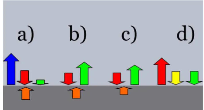
Figure 4. Energy budget near surface at different times: before
the onset of fog (a), after the onset of fog (b), before sunrise (c) and after sunrise (d). Long-wave radiative flux in blue, sensible heat flux in red, latent heat flux in green, ground flux in orange and short-wave radiative flux in yellow.
In the following hours, the air temperature grows, although at a progressively decreasing rate. There is a reduction in the ground flux that is compensated by a reduction in the latent flux, while the sensible flux does not show any substantial variation (Fig. 4c). After sunrise, the thermal profile within the fog layer becomes unstable. The vertical heat flux near the ground becomes positive and progressively grows. The net long-wave radiation continues being almost negligible. The ground flux is also nearly zero, because ground and air temperature are very close each other. The sensible heat flux has to be balanced by the small portion of solar radiation that reaches the ground and the latent heat flux that is now likely to point downwards due to the probable cessation of the evaporation (Fig. 4d).
At the upper level of the mast, the vertical heat flux is mostly positive from the onset of fog onwards. The analy-sis of the temperature and moisture records yields that there is a strong thermal inversion and an increase of specific hu-midity with height above the top of the fog layer. Both latent and sensible heat fluxes point downwards and converge with the in-fog upward flux. They all are balanced by a strong net long-wave radiative flux.
5 Conclusions
This paper presents the application of a wavelet method to estimate turbulent magnitudes in fog events. The analysis of turbulence is really useful when it is performed together with that of the other terms involved in the energy budget (ground flux and especially long-wave and short-wave radia-tive fluxes) and, ideally, with those of the water budget. This analysis contributes to improving the knowledge of the phys-ical mechanisms that are relevant in the fog evolution. Since the application of numerical weather prediction models to fog forecast has evidenced important shortcomings (Bergot et al., 2007) and other methods (e.g. statistical methods) have
34 E. Terradellas et al.: Analysis of turbulence in fog episodes not provided a general solution, it is especially important to
make available conceptual models that will assist forecast-ers in their practice. Nevertheless, prior to further studies, the deployment of additional instruments to get quantitative estimation of the terms should be considered.
It is not possible to state definitive conclusions after the analysis of a single case. Nevertheless, it can be pointed out that the vertical profiles within the fog layer and, therefore, the value and even the sign, of the turbulent fluxes can no-tably change along the different stages of the fog evolution. It is also especially remarkable that, at least in the first stages, when there are not significant radiative fluxes near the sur-face, if the ground flux is not very large, sensible and latent fluxes tend to cancel each other, a situation that is not com-mon in a clear atmosphere.
It is necessary to point out the singularity of the event pre-sented in this paper. An increase of the screen temperature after the onset of fog, attributed to the unstabilisation of the saturated layers and the movement of the thermal inversion from the ground to the top of the fog layer, is commonly observed (Roach et al., 1976). The particularity of the described case is that the fog layer deepens during several hours – at least until the sunrise – at a regular rate, causing a progressive increase of the low-level temperature that lasts for hours.
Edited by: A. M. Sempreviva
Reviewed by: T. Bergot and another anonymous referee
References
Bergot, T., Terradellas, E., Cuxart, J., Mira, A., Liechti, O., Mueller, M., and Nielsen, N. W.: Intercomparison of Single-Column Nu-merical Models for the Prediction of Radiation Fog, J. Appl. Me-teor. Climatol., 46, 504–521, 2007.
Bowen, B. M.: Improved wind and turbulence measurements using low cost 3-D sonic anemometers at a low wind site, Preprints of the 13th A.M.S. Symposium on Meteorological Observations and Instrumentation (7.4), Savannah, GA, 2005.
Duynkerke, P. G.: Radiation fog: a comparison of model simulation with detailed observations, Mon. Weather Rev., 119, 324–341, 1991.
Fuzzi, S., Facchini, M. C., Orsi, G., et al.: The Po Valley Fog Ex-periment 1989: an overview, Tellus, 44B, 448–468, 1992. Gultepe, I., Tardif, R., Michaelides, S. C., Cernak, J., Bott, A.,
Bendix, J., M¨uller, M. D., Pagowski, M., Hansen, B., Ellrod, G., Jacobs, W., Toth, G., and Cober, S.G .: Fog Research: A Re-view of Past Achievements and Future Perspectives, Pure Appl. Geophys., 164, 1121–1159, 2007.
Roach, W. T., Brown, R., Caughey, S. J., Garland, J. A., and Read-ings, C. J.: The physics of radiation fog I – a field study, Q. J. Roy. Meteor. Soc., 102, 313–333, 1976.
Terradellas, E., Soler, M. R., Ferreres, E., and Bravo, M.: Analysis of Oscillations in the Stable Atmospheric Boundary Layer Using Wavelet Methods, Bound.-Layer Meteorol., 114, 489–518, 2005. Welch, R. M. and Welicki, B. A.: The stratocumulus nature of fog,
J. Appl. Meteorol., 25, 101–111,1986.
Zhou, B. and Ferrier, B. S.: Asymptotic Analysis of Equilibrium in Radiation Fog, J. Appl. Meteor. Climatol., in press, 2008.