Dynamic Order Allocation for Make-To-Order
Manufacturing Networks: An Industrial Case
Study of Optimization Under Uncertainty
by
MASSACHUSET1 8 IN$STITU 1 KOF TECHNO'0LOYy
Gareth Pierce Williams
AUG'
B.S., University of California, Berkeley (2006)
LIBRARI E
Submitted to the Sloan School of Management
in partial fulfillment of the requirements for the degree of
ARCHIVES
Doctor of Philosophy in Operations Research at the
MASSACHUSETTS INSTITUTE OF TECHNOLOGY
June 2011
@
Massachusetts Institute of Technology 2011. All rights reserved.Al 1 .1//
A uthor... ...
Sloan School of MVanagement
%r-7 A
Certified by ...
May 20, 2011 Jernie Gallien Associate Professor of Management Science and Operations London Business School
Accepted by ...
Thesis Supervisor
\
I . Patrick Jaillet
Dugald C. Jackson Professor Department of Electrical Engineering and Computer Science Codirector, Operations Research Center
Dynamic Order Allocation for Make-To-Order
Manufacturing Networks: An Industrial Case Study of
Optimization Under Uncertainty
by
Gareth Pierce Williams
Submitted to the Sloan School of Management on May 20, 2011, in partial fulfillment of the
requirements for the degree of
Doctor of Philosophy in Operations Research
Abstract
Planning and controlling production in a large make-to-order manufacturing network poses complex and costly operational problems. As customers continually submit customized orders, a centralized decision-maker must quickly allocate each order to production facilities with limited but flexible labor, production capacity, and parts availability. In collaboration with a major desktop manufacturing firm, we study these relatively unexplored problems, the firm's solutions to it, and alternate approaches
based on mathematical optimization.
We develop and analyze three distinct models for these problems which incorpo-rate the firm's data, testing, and feedback, emphasizing realism and usability. The problem is cast as a Dynamic Program with a detailed model of demand uncertainty. Decisions include planning production over time, from a few hours to a quarter year, and determining the appropriate amount of labor at each factory. The objective is to minimize shipping and labor costs while providing superb customer service by produc-ing orders on-time. Because the stochastic Dynamic Program is too difficult to solve directly, we propose deterministic, rolling-horizon, Mixed Integer Linear Programs, including one that uses recently developed affinely-adjustable Robust Optimization techniques, that can be solved in a few minutes. Simulations and a perfect hindsight upper bound show that they can be near-optimal. Consistent results indicate that these solutions offer several hundred thousand dollars in daily cost saving opportu-nities by accounting for future demand and repeatedly re-balancing factory loads via re-allocating orders, improving capacity utilization, and improving on-time delivery. Thesis Supervisor: J6r6mie Gallien
Title: Associate Professor of Management Science and Operations London Business School
Acknowledgments
Foremost, I would like to thank my advisor, Jeremie Gallien, who made this work possible by introducing me to the problem, providing contacts and professional knowl-edge, and easing responsibility into my hands. I greatly appreciate his kind, just and wise guidance, which continued throughout my doctoral work.
Steve Graves and Cindy Barnhart, the other members of my thesis committee, imparted crucial feedback. John Foreman, who worked on a related project, aided me in many ways. Several employees at the firm motivating this work, especially Juan Correa, Spencer Wheelwright, and Jerry Becker, were instrumental in the acquisition of data and model development in this thesis.
This firm, the Singapore-MIT Alliance, research assistantships from Jeremie, and teaching assistantships funded my graduate eduction. It was an honor and a pleasure to teach with Jer6mie, Vivek Farias, Arnie Barnett, Dick Larson, Cynthia Rudin, and Jim Orlin. Cindy Barnhart, Dimitris Bertsimas, and Patrick Jaillet, as ORC codirectors, all provided superb advice throughout my doctoral candidacy. The ORC administrators, Laura Rose, Paulette Mosley, and Andrew Carvalho, went above and beyond helping.
My colleagues at the Operations Research Center, many of whom contributed
ideas to this thesis and are too many to list, were a great source of camaraderie, moral support, and intellectual stimulation. My officemates at the Operations Research Center, Alex Rikun, Ruben Lobel, and Jonathan Kluberg, made working at the office a pleasure. I give special thanks to Cristian Figueroa, Philipp Keller, Eric Zarybnisky, Michael Frankovich, Zachary Leung, Matthieu Monsch, Nikos Trichakis, David Gold-berg, Diana Michalek Pfeil, Jason Acimovic, Dan Iancu, Adrian Becker, Matthew Fontana, and Vishal Gupta. My companions, Ying Zhu and Deborah Witkin, were always there for me.
Lastly, I would not be who I am without the loving and everlasting support of my family.
Note on Confidential Information
So as to protect the firm's proprietary and confidential information, much of the data presented in this thesis has been changed to prevent access by competitors. Although specific values of many parameters vary from their true historical value, the relative values and qualitative results that we present still represent reality well.
Contents
1 Introduction 19
2 Case Study: Geo-manufacturing 2.1 The Supply Chain ...
2.2 Problem Scope and Definition ...
2.2.1 Planning . . . . 2.2.2 Execution ...
2.3 Understanding Factory Production Capacity ... 2.4 The Operations Center's Geo-manufacturing Strategy
2.4.1 Geographic Manufacturing Plans . . . . 2.4.2 Geo-move Execution . . . .
3 Literature Review
3.1 Production Planning and Control . . . .
3.1.1 Make-To-Order . . . .
3.1.2 Network Manufacturing . . . .
3.1.3 Dynamic Programming Solution Techniques .
3.2 Similar Implementations . . . .
3.3 Other Work on the Firm . . . .
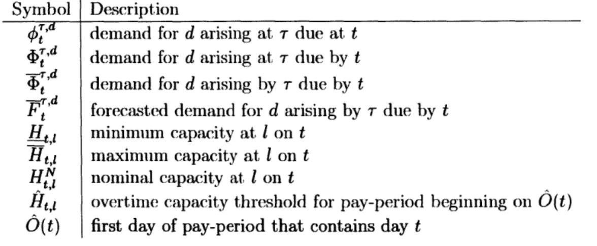
4 Execution Problem: Mathematical Formulation and Analysis 4.1 Mathematical Notation . . . . 4.1.1 Indices . . . . 23 . . . . 23 . . . . 26 . . . . 27 . . . . 3 1 . . . . 33 . . . . 38 . . . . 38 . . . . 4 1 45 . . . . 45 . . . . 46 . . . . 49 . . . . 50 . . . . 52 . . . . 53 57 58 58
4.1.2 Decisions . . . .
4.1.3 Costs . . . . 4.1.4 Data Parameters . . . . 4.2 Dynamic Programming Formulation . . . . 4.3 Simplifications . . . . 4.3.1 Product Differentiation, Availability an( Geo-Eligibility . . . . 4.3.2 Labor Shift Structure Details . . . . . 4.3.3 Managerial Concerns . . . . 4.3.4 Solution Approaches . . . . 4.4 Data Sources . . . . 4.4.1 Indices . . . . 4.4.2 Cost Data . . . . 4.4.3 Demand and Labor Data . . . . 4.5 Demand Structure . . . ..
4.5.1 Data Analysis and Estimation . . . . . 4.5.2 Correlation Structure . . . . 4.5.3 Additional Adjustments . . . . 4.5.4 Forecast Error . . . . 4.5.5 Validation . . . . 4.6 Policies . . . . 4.6.1 Greedy Policy . . . . 4.6.2 Historical Policy . . . .
4.6.3 Linear Programming Policy . . . . 4.6.4 Perfect Hindsight Policy . . . . 4.7 Evaluation Criteria and Simulation Structure.
4.8 Simulation Results and Insights . . . .
. . . . 59
d Transfer Parts, and
60 61 63 64 65 67 68 69 70 71 72 75 76 81 83 85 88 90 91 95 96 100 101 . . . . 104 5 Execution Problem: Implementation
5.1 Introduction . . . . . . . .. 10
115 115
5.2 Model Development . . . . . 5.2.1 Qualitative Description . . . . 5.2.2 Notation . . . . 5.2.3 Production Constraints . . . . 5.2.4 Parts Constraints . . . . 5.2.5 Labor Constraints . . . . 5.2.6 Factory Bottlenecks . . . . 5.2.7 Costs . . . . 5.2.8 Complete Formulation . . . .
5.2.9 Practical Challenges and Solutions
5.3 Results and Insights . . . .
5.3.1 Results from Fall 2008 . . . .
5.3.2 Results from Spring 2009 . . . .
5.3.3 Conclusions . . . .
6 Planning Problem: Formulation, Implementation, 6.1 Nominal Formulation ...
6.2 Robust Formulation ...
6.2.1 Robust Optimization Literature ...
6.2.2 Uncertainty Model ...
6.2.3 Affinely-Adjustable Production . . . . 6.2.4 Robust Counterparts . . . .
6.3 Extension to Multi-Product Setting . . . .
6.4 Implementation Details . . . .
6.5 Validation and Analysis Methodology . . . .
6.6 Results and Insights . . . .
7 Conclusion
A Glossary of Terms and Abbreviations
116 . . . . 116 . . . . 120 . . . . 121 . . . . 125 . . . . 127 . . . . 132 . . . . 134 . . . . 136 . . . . 141 . . . . 144 . . . . 144 . . . . 154 . . . . 157 and Analysis 163 . . . . 164 . . . . 170 . . . . 171 . . . . 174 . . . . 177 . . . 181 . . . . 184 . . . 185 . . . . 188 . . . . 190 197 201
List of Figures
2-1 Maximum weekly production output of TX. ... 35 2-2 Maximum weekly production output of TN. . . . . 36
2-3 Maximum weekly production output of NC. . . . . 37
2-4 The firm's geoman, or geographic manufacturing, map partitions the United States into thirteen geographic regions (Alaska not shown), represented by different colors. Regions are assigned to factories, indi-cated by the bold lines; by default, factories produce orders that are to be shipped to the geographic regions that they are assigned. For each factory, its location, the percent of U.S. demand assigned to it, and additional international destinations are given in text. This particular allocation was used in Fall 2006 and was typical for most quarters from
2006 to 2008. . . . .. -. . - - - . 40
4-1 Example of the Lookahead spreadsheets used by the firm's Operations C enter. . . . . 73 4-2 Relative Optimality Gap (4.32) of each policy on each instance W in
increasing order of CPBPH. ... 106
4-3 The lateness quantity uq,p,, for several values of the lateness penalty
P on a particular instance w that displayed significant order lateness, for policies H, LP, and PH. . . . .. . . . 110
4-4 A scatter plot of the relative optimality gap (4.32) against the forecast error f for the LP policy. . . . . - . . -. . . 111
5-1 The maintenance schedule, convenient buttons for updating, and color codes used to help employees keep data up-to-date. . . . . 142
5-2 User interface to easily toggle sets of constraints on and off. . . . . . 143
5-3 Planned and actual shift lengths for each factory and shift on
Septem-ber 29th, 2008 with NCLL enabled and 100% of forecast. . . . . 147 5-4 Optimal shift lengths for each factory and shift on September 29th,
2008 with NCLL enabled and 100% of forecast, when labor is restricted
to no flexibility (flex), some flex, and full flex. . . . . 148
5-5 Cumulative production and labor capacity (as a fraction of total
pro-duction during the horizon) at each factory over the horizon starting on September 29th, 2008 with 150% demand and NCLL enabled, for the firm's actual solution (a) and the optimal solution with full labor flexibility (b). . . . . 151 5-6 Optimal solution's suggested order moves for 100% demand, inflexible
labor, NCLL Enabled, starting on September 29th, 2008. Each factory has a color; each state is colored to match the factory that had the most orders moved from or to it from that state. More intense colors indicate higher portions of that states desktops being moved. . ... 153 5-7 Planned, actual (historical), and optimal shift lengths for each factory
and shift for the horizon starting on April 23rd, 2009. . . . . 156 5-8 Cumulative production and capacity (as a fraction of total production)
at each factory over the horizon starting on April 23rd, 2009. . . . . . 158 5-9 Optimal solution's suggested order moves when the horizon starts on
April 23rd, 2009. Each factory has a color; each state is colored to match the factory that had the most orders moved to it from that state. More intense colors indicate higher portions of that state's desktops being moved. . . . . 159
6-1 The Hockey Stick Effect - The historical production capacity at TX,
TN, and NC during
Q3
2007 and the model's theoretical productioncapacity are depicted rising throughout the quarter in three intervals. 168
6-2 User interface for the planning model, including controls to make
pop-ular changes to input parameters and easily access the model output. 187 6-3 Maps of the United States colored by which factory produces the most
desktops for that destination state in scenarios (a), (b), (d), and (e), for both Lines of Business. TX is red; TN is green; NC is blue. . . . . 196
List of Tables
2.1 The name, location, first year of production (start), and final year of production (end) of relevant production facilities. . . . . 25 4.1 Mathematical notation for indices . . . . 59 4.2 Mathematical notation for decisions, all in units of number of desktops. 59 4.3 Mathematical notation for cost parameters, all in units of U.S. Dollars
($) per desktop. . . . . 60 4.4 Mathematical notation for data parameters, all in units of desktops
other than the
O(t)
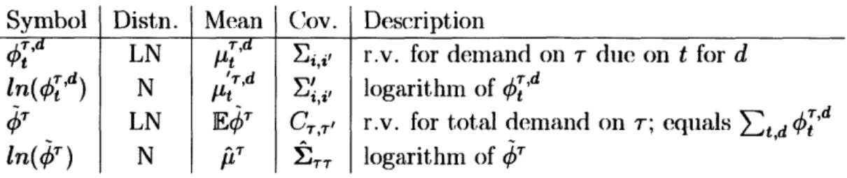
which is a day. . . . . 61 4.5 A brief description of the source of relevant data parameters. . . . . . 70 4.6 Mathematical notation for demand parameters, in units of desktops.Distributions (Distn.) are either Normal (N) or Log-Normal (LN). The index i represents a triplet (t, r, d), Cov. is the covariance, and r.v. means random variable. . . . . 78 4.7 Regression of ln(47) (log desktops) for ^ with Weeknumber and
De-mand k days ago. R2 = 0.941. . . . .. . . 79
4.8 Regression of ln(qV) (log desktops) for - used in demand generation. R2 = 0.939. . . . .. -. . . - - - -. 79
4.9 Demand model validation metrics for various values of 0 and a. Note that
#o
= 0.0277 and (a, N) is chosen to zero M4. ... 904.10 Dimensions to aggregate results by for evaluation. . . . . 103 4.11 95% confidence intervals on total Cost-Per-Box by policy in dollars per
4.12 95% confidence intervals on the total quarterly cost z, by policy in
millions of dollars. . . . . 106
4.13 Cost-Per-Box by policy and cost category in dollars per desktop. . . . 107
4.14 Cost-Per-Box by policy and cost category in dollars per desktop when demand is correlated via a = 16%. . . . . 108
4.15 Distribution of production among factories, "U*, for each policy. UYpp . . 112
4.16 The excess capacity " - 1 at each factory I and the total excess capacity ",P - 1 under each policy. . . . . 112
4.17 The number of destinations that have more than 1 or 1000 desktops produced for it by each factory for each policy. . . . . 113
4.18 Average overtime capacity (in units of desktops) per quarter for each policy at each factory. . . . . 113 5.1 Average daily difference between actual and optimal quantities from
September 7th to October 14th, 2008, with NCLL enabled for several scenarios with varying labor flexibility (Flex.) and forecasted demand. 149
5.2 Outbound shipping cost of already known orders for Actual and
Op-timal policies, by factory and line of business, for the horizon starting on September 29th, 2008 . . . . 154
5.3 Average daily quantity of late desktops, shipping cost, and labor cost
for the historical and optimal solutions in the Fall of 2009. . . . . 155 6.1 Relative inbound, outbound, and labor cost savings for each scenario
as a percent of the cost of baseline scenario (a) in
Q4
2007. . . . . 190 6.2 Permanent labor capacity at each factory as a percent of the baselineChapter 1
Introduction
This thesis addresses production planning and control problems encountered by make-to-order manufacturers that have multiple production facilities. As rapid advances in technology improve the availability of information, global supply-chain controls are being developed to improve market responsiveness to shifting consumer demands. In make-to-order network manufacturing, firms must use automated controls to quickly and efficiently allocate thousands of custom orders to multiple manufacturing facili-ties.
This work is motivated by and performed in collaboration with a particular, large, make-to-order desktop computer manufacturing company, hereafter referred to as "the firm," that needed such controls. The firm is a $61B annual revenue corpora-tion, based in Austin, Texas, United States, that designs, manufactures, sells and supports computer-related products. In North America, the firm manufactures hun-dreds of thousands of consumer and corporate desktop computers each week. Rather than selling via typical retail channels, the firm developed an innovative make-to-order and direct factory-to-customer shipping business model, which many other companies have now adopted. This business model provides great value to customers by tailoring products to their desires and reduces inventory requirements by assembling finished goods Just-In-Time. However, this business model makes outsourcing final assembly of products difficult and increases direct labor and shipping costs. In North America, the firm produces desktops from multiple factory locations to improve delivery lead
times, reduce shipping costs, and mitigate the risk of losing all manufacturing capabil-ity. Uncertainty regarding the quantity, timing, and geographic destination of future orders for desktops complicates the decision of how to allocate orders to factories and adjust production capacity to match demand. Because computer manufacturing is one of the most rapidly growing and competitive industries with products that are becoming more difficult to differentiate, cost-advantages are critical to gaining a competitive advantage. The firm's flexible, complex, and cutting-edge supply chain presents an excellent opportunity to employ optimization-based solution techniques in an industrial setting.
The first major contribution of this thesis is exposition of this industrial problem which has received little attention in the literature. Chapter 2 presents the business problem faced by the firm and its innovative and evolving supply chain configuration,
illustrating a problem with several sets of industrial data that requires further research and setting the context for the remainder of the thesis. The fundamental question posed in this problem and answered by this thesis is "Which desktops should be built, when and where?" Intricacies of the problem, its associated challenges, and the firm's approaches to solving it are discussed in detail. Chapter 3 reviews the relevant academic literature, including production planning and control in make-to-order and network settings, optimization-based solution techniques, similar industrial studies, and other work related to the firm.
Chapters 4, 5, and 6 contain the second major contribution of this work: three distinct models of the problem which incorporate the firm's actual data, testing, and feedback, discussions of challenges to optimization modeling in practice, and actionable solutions and insights. Analysis of these models demonstrates credible and realistic cost savings opportimities from optimization-based solutions. In all of these models, decisions include producing various desktops at factories over time and determining the appropriate amount of production capacity. The objective is to minimize the sum of several relevant supply-chain costs, including factory-to-customer shipping costs, the cost of labor that is used directly to produce the desktops, and the cost of poor customer service. Emphasis is placed on model realism and usability.
Several important questions are addressed in each of these chapters. How can we model the firm's problem mathematically? What choices are appropriate when balancing model tractability and realism'? What challenges can be encountered when using mathematical optimization techniques to solve an industrial problem in prac-tice? Compared to the firm's historical decisions, can mathematical optimization leverage the firm's manufacturing network to reduce relevant supply chain costs and improve customer service? If so, by how much and by making what decisions? Should the firm be producing orders in different factories or at different times? What is the appropriate amount of capacity to have at each factory? Can customer service be improved by satisfying more orders on time? How confident can we be in our answers to these questions?
In Chapter 4, the problem is formulated mathematically as a Dynamic Program-ming problem and demand is analyzed and modeled in great detail. A simulation study of various solution policies shows that a rolling-horizon, certainty-equivalent, linear-programming policy performs near-optimally, improving upon the firm's his-torical policy by several hundred thousand dollars per day.
In Chapter 5, the same problem is addressed deterministically by a large Mixed Integer Linear Program (MILP) with many details that were necessary for implemen-tation at the firm but too intricate or unintuitive for the in-depth analysis of Chapter 4, exposing many issues and insights that arise when using optimization in practice. Analysis of the solution to the MILP indicates similar potential cost savings of several hundred thousand dollars per day relative to the firm's actual decisions.
Chapter 6 studies the same problem but plans for production over the next quarter-year rather than the next few days. Another MILP is developed, incor-porating the cost to ship parts from suppliers to factories and decisions regarding how much staff to hire at each factory. Because demand data was limited and solu-tions suggested drastic reducsolu-tions in labor levels, Robust Optimization techniques are introduced, including discussions of how to model uncertainty appropriately and tech-niques to maintain tractability. Results demonstrate that, even under extreme levels of protection against uncertainty, optimization-based solutions can provide similar
cost savings of several hundred thousand dollars per day.
We coalesce these results and insights in Chapter 7, our conclusion. Many firms now face difficult decisions in a make-to-order network manufacturing environment. This thesis presents a thorough and grounded discussion of one such industrial prob-lem. Realistic and tractable modeling choices, which often go without much discus-sion, in addition to substantial financial impact, are necessary for optimization-based solutions to be used in practice. Consistent and data-driven results show that these controls can provide significant cost savings by dynamically allocating orders among production facilities to continually re-balance factory loads. The insights gained from thoroughly studying this firm's problems are readily applicable to other firms facing similar production planning and control problems in make-to-order manufacturing networks.
Chapter 2
Case
Study: Geo-manufacturing
This chapter describes the challenging production planning and control problems that were faced by the firm between 2006 and 2010 and are addressed in the remainder of this thesis. In §2.1 we describe the relevant history of the firm's supply chain, providing the problem framework. The problems are stated in §2.2. Further context is provided in the summary of several interviews in §2.3 which illustrate the firm's production capacity and labor force limitations at each factory. The solution that the firm was already using and provides the historical baseline for our study is described in §2.4.
2.1
The Supply Chain
The firm develops, assembles, sells and supports computers as well as related products and services. The firm is well known for its brand-name products and supply-chain innovation, shipping more than 110,000 computers every day to customers in over 180 countries. According to its website, in the third quarter of its 2011 fiscal year (ending October 29, 2010), the firm had a revenue of $15.4 billion, an operating income of $1.02 billion, a net income of $822 million, and earnings per share of $0.42.
The firm's unique and ground-breaking supply chain began in 1984 when it was founded in Austin, Texas, USA based on the idea that selling computers directly to the final customers would enable the best satisfaction of customer needs. Bypassing the
wholesalers and retailers, which are common in other computer distribution channels, allowed the firm to let customers configure orders to their own specifications and conferred greater control over its supply chain. Whereas most personal computer vendors must forecast demand and to-stock, the firm's direct-sales and build-to-order business model allow it to have excellent performance in inventory turnover, overhead, cash conversion, and return on investment. Although the firm relies on outside suppliers and contract manufacturers to provide many components of its products, it performs the majority of final assembly for desktops itself. Instead of owning its own parts inventory, suppliers own and manage parts in Supplier Logistics Centers (SLCs) near each of the firms factories; every computer the firm builds has already been sold before the firm owns the parts, a new and enviable business model for the computer industry. By having such close relationships with both customers and suppliers, the firm had an immense amount of information, allowing them to quickly respond to customer demand. However, the direct-sales model requires quick responsiveness in manufacturing capability and the information technology to support swift order-fulfillment. Hence, the firm must maintain excess production capacity to deal with demand volatility and hedge against significantly higher outbound shipping costs, striking the correct balance of production at each factory over time.
Orders are configured and placed in-person, by phone, or via the firm's web-site. Material Requirements Planning (MRP) software, combined with supervision from the firm's Operations Center and factory managers, determines when and where desktops will be assembled; these decisions are the crux of what we study. Every two hours, supplies are then requested from nearby vendors for orders that the MRP system determines should be built in the next few hours; vendors have two hours to deliver those parts from the SLC. The factory then puts the parts for each desk-top into kits, assembles the hardware, loads software, and tests basic functionality of these computers, using a substantial amount of human labor. The computers are then automatically packed in boxes that are later shipped from the firm's factories directly to consumer's doorsteps via third party logistics providers. This thesis focuses on the decision of when and where each desktop computer should be assembled.
Name Location Start End TX Austin, TX, USA 1984 2008 TN Nashville, TN, USA 1999 2009 NC Winston-Salem, NC, USA 2005 2010
JM San Jeronimo and Juarez, Mexico 2009 Present
Table 2.1: The name, location, first year of production (start), and final year of production (end) of relevant production facilities.
The firm's North American manufacturing network has evolved significantly. In 1984, the firm was founded in Austin, Texas (TX), where all manufacturing took place until 1996. In 1999, in order to increase production capacity, reduce the cost and lead-time of shipping directly to customers, and to reduce the risk of a disaster destroying all of its production capability, the firm opened a manufacturing facility in Nashville, Tennessee (TN). In 2005, it opened a third United States manufacturing facility in Winston-Salem, North Carolina (NC), where it received an incentive package "worth $240 million over 20 years from local and state governments" [Lad09] in exchange for meeting minimum employment targets. As demand for computers shifted toward notebooks, as the firm began selling via retail channels, and as investors pressured the firm to cut costs, starting in 2008, the firm began to terminate desktop production in its United States manufacturing facilities [SchO8]. The firm ended the manufacturing of new non-server desktops in Texas in 2008, in Tennessee in 2009, and in North Carolina in 2010. In 2009, it began outsourcing North-American desktop production to another firm with factories located in Mexico. Table 2.1 details the firm's North American manufacturing facilities, giving the names we refer to them by throughout this thesis, their geographic location, and the years they began and ended production. This thesis focuses on desktop computer assembly in North American markets between September 2006 and April 2009, before the firm began retail distribution in North America, when it used a primarily build-to-order business model. At the time, it had two major desktop Lines of Business (or product categories), which we refer to as consumer desktops and corporate desktops. The consumer oriented desktop line focused on value, reliability, and modularity. The corporate desktop line, focused on
longevity, reliability, and serviceability. In the time of this study, the firm
assem-bled nearly 150,0(X) consumer desktops and 100,000 corporate desktops for customers
across North America each week in two or three of its North American factories. The firm's North American customer base was distributed across the continent. The in-ternational nature of shipping to Mexico and Canada limited the production for most non-U.S. based customers to TX and TN, respectively. However, orders from across the United States were typically eligible to be built in almost any factory.
Having multiple factories capable of serving the same customer base with a Make-to-Order business model, enables much more dynamic production decisions than typ-ical. An identical order made one day later or from a few miles away can easily be built in a different factory. However, the immense number of possible options and the complex dynamics of the system make such production decisions difficult. As shown
by the following work, Operations Research techniques can help maintain efficient
op-erations in such a dynamic production environment. As discussed in §3.2, although the work outlined below analyzes a supply-chain that no longer exists, many compa-nies, often in other industries, have similar supply-chain configurations and should find this study useful. The Operations Center faced the difficult problem of deter-mining which orders should be produced in which factories and at what times. This thesis addresses that problem.
2.2
Problem Scope and Definition
We began working with the firm's North-American Operations Center, responsible for centralized supply-chain coordination in North America, in 2006. The Operations Center was responsible for assigning demand for various desktops with varying due-dates, parts requirements, and shipping destinations across the continent, to the three active manufacturing facilities, which have various supply and manufacturing capacities. Although the Operations Center had developed heuristics to handle these tasks, it was unsure of their efficacy. The fundamental question answered by this thesis is "Which desktops should be built, when and where?"
At the time, the firm made decisions regarding this at three levels or scopes. At a strategic level, with a horizon of about three to twenty years, the firm's senior management decided to open or close assembly facilities in different locations, as described in §2.1; we do not address this problem. At what we call the planning level, the Operations Center planned production, staffing, and parts-sourcing targets for each factory for a quarter-year or more. At the execution level, which concerns
day-to-day operations, looking at most two weeks into the future, factory managers
and the Operations Center determined when and where each order is fulfilled and how long hired labor would be needed on the factory floor. This thesis focuses on the planning and execution problems, assuming that the factory locations are fixed but
that production and labor-capacity decisions must be determined.
2.2.1
Planning
In order to inform parts supply decisions and factory staffing decisions, the firm plans its production for the next quarter (or occasionally year). Forecasts1for that quarter's sales volume, for each major Line of Business, were distributed among each week of the quarter based on historical percentages. The Operations Center, being responsible for production decisions, assigns this forecasted demand to different factories. Other groups within the firm then procure parts from vendors based on these production targets and factory managers hire sufficient labor to meet these production plans. Although the Operations Center does not make labor and parts sourcing decisions directly, it does consider the implications of its production decisions on other parts of the supply chain. In the planning problem, the major decisions that the firm plans for are 1) the volume of demand for various products that each factory will serve in each week, along with the associated production and backlog levels, and 2) the amount of labor necessary to serve that demand.
In the production of a desktop, parts components are assembled into into final
1We did not investigate alternatives to the firm's forecasting method, as it incorporates much
beyond the scope of our project, including strategic marketing decisions and executive desires. How-ever, we do analyze forecast data available to the Operations Center.
products. The firm shares forecasts of future demand with its parts suppliers who then manufacture and ship to the firm what they think will be a sufficient supply of parts. Although the suppliers own and manage the parts until just a few hours before assembly, the firm makes routing decisions regarding which purchased parts should
be delivered to each factory about a month in advance of their arrival to the United
States. Parts arrive from mostly Asian suppliers in Long-Beach, California, and are shipped via truck or train to each of the Supplier Logistics Centers near the firm's manufacturing facilities. Foreman
[For08]
addresses the problem of routing these parts for the same firm and its many complexities in great detail. The cost to ship various parts to different factories largely depends on the number of parts that fit on a shipping pallet, the mode of transit used, and the distance to the factory. Because parts routing decisions are made by another department within the firm and heavily depend on information that becomes available after production plans have been made, the Operations Center considers the implications of its production decisions on parts routing by using the average cost to ship parts to each factory, which is referred to as the inbound shipping cost.Customers can choose how quickly they would like their order to be fulfilled from a set of limited options (e.g. 2, 3, 5, or 7 days) which, along with the Operations Center's choice of manufacturing location, determines the due date by which those orders must be produced. Failing to produce an order by its due date is considered poor customer service and can incur significant costs to the firm. The costs include order cancellations, contacting or being contacted by customers, concession of other valuable goods to appease customers, reduced likelihood of future purchases from the firm, and expedited third-party shipping. Dhalla [Dha08 analyzes these costs in great detail.
In a Make-to-Order business model, production for orders can only occur after customers configure those orders. The firm must produce these orders in the few days between when the order is made and when it is due. To do so, it must schedule sufficient capacity to assemble the desktops. Production capacity is limited by two expensive resources: 1) the physical layout and machinery of the factories and 2)
the amount of labor available to operate the factory. The physical layout includes
space for workers to assemble desktops and store work-in-progress (WIP) inventory
on the factory floor and space to keep not-yet-shipped but finished goods. Machinery includes equipment that burns software onto hard-drives, tests machine functionality, boxes desktops, labels boxes, and sorts and shrink-wraps them for shipping. Purchas-ing additional machinery or changPurchas-ing the factory layout was beyond the scope of the Operations Center's decision making. However, the Operations Center did determine machinery utilization by assigning orders to each facility and thereby influence the amount of labor available to operate the machinery.
Producing desktops at the firm's factories requires a significant amount of direct labor to gather the correct components (called "kitting") and assemble them, which scales in proportion to production volumes. Labor varies in several ways that affect production capacity. The number of workers and quality of workers determines how quickly parts are gathered and assembled and therefore the rate that desktops can
be assembled. Production in any period is limited by this rate multiplied by the
amount of time that these workers operate the factory. Because limited space for WIP is available, as desired in a Make-to-Order environment, a steady flow of material must be supplied to the machinery; hence, another limit on production is the rate that machinery can process desktops multiplied by the amount of time that workers operate the factory. As such, the number and quality of workers as well as the amount of time they work are critical capacity decisions.
Factories employ both permanent and temporary laborers. Permanent hires tend to stay at the firm for at least a few months if not many years and can take weeks to recruit. Temporary laborers are available within a few days notice and may be hired for just one day or for a few weeks but are often less. skilled at production tasks. The firm limits the number of temporary workers to be less than some fraction of permanent workers at each factory to both ensure quality and to be able to ensure enough people have appropriate training for each task. Although permanent labor tends to be more expensive and less flexible in quantity, their expertise is necessary for quality.
The workers who perform this direct labor are assigned to work-teams at each factory that operate shifts of varying lengths and frequencies. Typically, a work-team will be scheduled to eight-hour shifts on five days of each week, or ten-hour shifts four days per week, or twelve-hour shifts three days per week. These planned shift lengths and frequencies are often referred to as nominal or straight-time hours. Although the firm plans this shift structure, factory mangers often deviate from it and ask work-teams to either work longer shifts or go home early. Usually, all workers in a work-team will end their shift at the same time. If a work-team works less than their nominal number of hours in a pay period, the firm almost always pays the workers for all of the nominal hours anyways, making it a sunk cost. However, if a work-team works more than their nominal number of hours in a pay period, the firm pays an additional cost for each overtime hour. For instance, if a work-team has five eight-hour shifts per week, it will have eighty straight-time eight-hours per pay period. If the work-team works less than eighty hours, it is still payed for eighty straight-time hours. If it works for eighty-five hours in those two weeks, it is payed for eighty straight-time hours and five overstraight-time hours. Each shift has a minimum and maximum length which limits the amount of WIP they can kit, assemble and pass downstream to more automated machinery.
After a desktop has been assembled, loaded with software, tested, and boxed, it is shipped directly to the customer via a third party logistics provider. Although the customer may pay a shipping-fee to the firm at the time of ordering, the firm pays the third party logistics provider different prices based on both the manufacturing location and the customer's shipping address, which we typically call the destination, in addition to factors such as speed of delivery and the size or weight of each box. The choice of where each order is produced and what destination it is shipped to is a significant factor in how much the firm pays to third party logistics providers, which we call the outbound shipping cost. Because the firm ships desktops from its factories to customers in small quantities, preventing economies of scale, the outbound shipping cost can become relatively expensive and important in determining where an order should be produced.
The planning problem faced by the firm's Operations Center is determining how to allocate demand for a quarter-year's worth of desktops to the firm's North American production facilities. It should consider inbound shipping costs, outbound shipping costs, the cost of direct labor, limitations of the labor force, constraints on produc-tion capacity, and possibly uncertainty in demand and how demand differs from its forecast. Balancing all of these factors simultaneously can be difficult and misman-agement can cost several hundreds of thousands of dollars per day.
2.2.2
Execution
All of the issues encountered in planning problem, other than changing the size of the
labor force, apply to the execution problem as well. Nonetheless, as the execution problem considers day-to-day operations, it contains many more fine details that must be considered. Some orders can only be satisfied by particular factories for a variety of reasons, including parts availability, labor expertise, customer requests, and legal issues. Scheduling the labor force become much more complex. Many more details are known about orders that have been configured and should be incorporated into
the decision-making process.
In the execution scope, daily decisions are made regarding which orders are built in each factory and the how long each work-team operates the factory at its pre-determined staffing level. Each day, from a backlog of available-to-build (ATB) orders from the recent past, often zero to four days worth of production, the Operations Center must decide whether to leave orders where they were assigned by the default plan or 'move' them from one factory to another. Further complicating this, more orders will be made and become due in the near future. The rate at which each work-team can produce desktops has already been determined by past staffing decisions, but the length of time they spend producing desktops has yet to be finalized. With projections for future sales and schedules for labor availability over the next two weeks, decisions must be made for what is to be done today. Factories then execute those decisions by producing the associated desktops.
spec-ify the quantity and type of desktops, necessary parts, due-date, shipping destination,
and which factories can produce them. Little is known about orders that have yet to be configured other than forecasts of the total sales volume each day. As in the planning problem, orders must be fulfilled between the time that they are configured and the time that they are due; if an order is not fulfilled until after its due-date, customer service deteriorates. Because the volume, parts requirements, due-dates, shipping destinations, and eligibility of future orders is uncertain, making production decisions can be difficult. Large volumes can either force factories operate longer and at greater expense than planned or delay orders past their due dates. Producing too much too early can leave factories starved for work when sales volumes are low, wasting valuable resources such as labor that will be paid for anyway. Nonetheless, factories can pool some of their capacity by compensating for imbalances between them.
The Operations Center must decide which orders to satisfy immediately and which orders should be delayed until a later date or moved to other factories. Because bulky, heavy desktops are expensive to ship directly to customers, the choice should include considerations for outbound shipping costs. These decisions also alter the length of each work-team's shift which can cause non-trivial scheduling complications. The duration of most shifts is limited to an interval of time. In order for a shift to be extended beyond its nominal length, advanced notice must be given to the work-team one to two days in advance, depending on the day of the week. Similarly, work-teams can be called in for new shifts or added to existing ones. If a shift is extended long enough, it may overlap with another shift, which has different ramifications for physical bottlenecks and labor productivity; machines and space are still limited to the same production rate, but desktops can be kitted and assembled almost twice as fast. The number of hours worked so far in each pay period is tracked and can be used to predict the cost of overtime. Concerns about fairness in balancing the workload of each factory must be considered. Not only must the lengths of the current days' shifts be adjusted, but estimates of future shift lengths are important information for managing the workforce.
The Operations Center must assign orders to be built at locations that have parts available. Alternatively, parts can be transferred between factories to match demand within a few days through multiple modes of transit, including a regularly scheduled shuttle and trucking services that are available on-demand. Checking the availability of parts can be difficult. Although suppliers frequently update the firm about what parts are available in the Supplier Logistics Center and what deliveries can be expected over the next few weeks, variability in the time to delivery, substitution of parts for each other, and data inaccuracies complicate matters. Because the parts have already been routed to each factory's Supplier Logistics Center, inbound shipping costs are no longer relevant. However, part shortages occasionally occur at individual factories and throughout the network and can cause many orders to not be satisfied on-time which is costly.
The execution problem faced by the firm's Operations Center is determining which factories should satisfy each order, if at all, in the next twenty-four hours, accounting for how this affects production over the next two weeks. It should consider outbound shipping costs, the length of each work-team's shift, its impact on capacity and direct labor costs, and parts availability. Because demand and parts supply vary from planned values, the firm must repeatedly adjust its production tactics. Accounting for all of these factors simultaneously can be difficult but is critical to the firm's ability to operate and can be worth several hundreds thousands of dollars per day.
2.3
Understanding Factory Production Capacity
Given the importance of each factory's physical layout, machinery, and labor force, in
2006 we interviewed employees at each factory to understand that factory's production
capacity. In some cases, multiple interviews and email correspondence were necessary to confirm the accuracy of the following details. Although many of the particular numbers described below changed throughout the course of this study, the constraints described continued to be exemplary of the limitations on production at the firm's factories and are referred to throughout this thesis.
TX Production Capacity
In [Fel06], Jennifer Felch, one of the managers at TX, the main desktop production facility in Texas, described the limitations on production capacity at TX. TX has six "kit lines" that gather parts into kits and assemble desktop hardware. Each kit line can produce up to 250 consumer desktops per hour or 300 corporate desktops per hour, or any mix of the two at those rates. However, only two of these six kit lines can assemble consumer desktops because the parts for consumer desktops are stored in only two kitting areas for this more customized Line of Business. These are physical constraints of the factory layout.
According to [Fel06], the labor shift structure also constrains productivity at TX. The default schedule has two work-teams operate two shifts per day that last eight hours per shift and have about 6.25 productive hours per shift, for five days each week. The most this schedule could be extended to is two shifts per day that last eleven hours per shift and have nine productive hours per shift, for seven days per week; this cannot be maintained indefinitely but can be done when facing extraordinarily high demand. Furthermore, most scheduled shifts must last at least six hours. Each work-team has up to eighty straight-time hours per two weeks and is paid overtime wages for any time spent on the factory floor in excess of eighty hours in a two-week pay-period.
The maximum weekly production output of TX, based on physical bottlenecks and the shift structure, is depicted in Figure 2-1. The inner region of the figure indi-cates production mixes of consumer and corporate desktops that are feasible without extending shifts beyond the default schedule; the outer region is possible by extending shifts. The number and skill of available workers for these shifts can further constrain production; the firm tracked this by estimating the average Units-per-Hour (UPH) production rate for each work-team; combined with the length of a shift, UPH pro-vides a reliable estimate of the number of desktops that a work-team can produce during its shift.
Thousands of Corporate
Desktops - possible during nominal hours
375
6 production Ines - possible by extending shifts
225-
165-105
At most 2 Consumer fines Thousands of
0 P Consumer
o 45 90 Desktops
13
Figure 2-1: Maximum weekly production output of TX.
TN Production Capacity
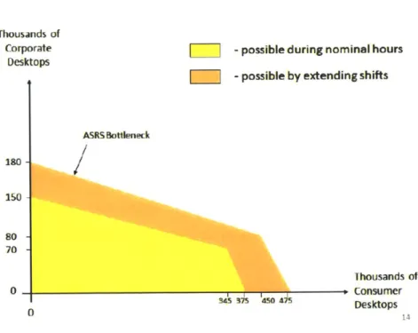
In [Dol06, DH06], Eric Dolak, an employee at TN, and Michael Hoag, an Operations Center employee, describe limitations on production at TN, the firm's factory in Nashville, Tennessee. According to engineering specifications, TN has seven produc-tion lines that can produce 400 units per hour, yielding a total 2800 UPH, independent of product mix; however, if six or seven production lines assemble only consumer desk-tops, capacity drops to 2150 or 2250 UPH, respectively. Although each production line only builds one Line of Business at a time, over the course of a week or even shift, production can be smoothed to achieve any mix of products.
In addition to the number of production lines, boxing assembled desktops in prepa-ration for shipping is a major physical bottleneck at TN. Large corporate orders that must be shipped together can consume most of the storage space in the the Automated Storage and Retrieval System (ASRS). At most 200 boxes can be work-in-progress (WIP) inventory before the two typically corporate desktop production lines must
shut down; this 200 desktop build-up of WIP can be cleared when work-teams pause for a break every four hours. Given the rate that WIP builds for each Line of Business at TN, we can compute how the ASRS constrains the production mix.
The labor structure at TN includes two work-teams that work five eight-hour (7.3 productive hours) shifts per week and one work-team that works four ten-hour (9.3 productive hours) shifts per week. Shifts can be extended to two work-teams on four ten-hour (9.3 productive hours) shifts and two work-teams on three twelve-hour
(10.75 productive hours) shifts. Minimum shift lengths varied by shift. The default
shift length also determined the number of hours until overtime began.
The implications of the number of production lines, the ASRS bottleneck, and the shift structure on TN's maximum weekly production output are depicted in Figure 2-2. Labor availability can further restrict this.
Thousands of
Corporate - possible during nominal hours
Desktops
I
= - possible by extending shifts
ASRS Bottleneck 150-80 -70 -Thousands of 0 consumer 0 34S S 450 47 Desktops
NC Production Capacity
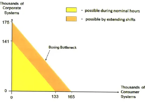
Rebecca Fearing and Sean Holly, in [FH06], describe NC, located in Winston-Salem, North Carolina, as being the newest and most flexible North-American production facility. Because only 900 orders can be labeled per-hour, boxing is the biggest bottle-neck at NC, limiting it to 900 UPH if producing solely consumer desktops and 1096
UPH if only producing corporate desktops, whose orders tend to contain multiple
desktops. Over the course of this study, the capacity of NC increased to almost 1400
UPH. By this point, the production rate at NC was independent of the product mix. NC has three work-teams, one working four ten-hour (8.75 productive hours), one
working five eight-hour shifts (6.75 productive hours), and one working three twelve-hour (10.75 productive twelve-hours) shifts on weekends, each week. The first shift can be extended by one hour each day and the second can be extended by four hours each day. Minimum shift lengths varied by shift. The default shift length also determined the number of hours until overtime began. Figure 2-3 depicts the maximum weekly production output at NC if it is fully staffed.
Thousands of
Corporate - possible during nominal hours
Systems
[751
L - possible by extending shifts175 141-Boxing Bottlneck Thousands of 0 Consumer 0 133 165 Systems
By 2008, when we developed and implemented a model to solve the problem
at the execution scope, the NC factory had added "lean lines" in addition to the already existing conventional production lines. These lean lines focused on building specific high-volume products efficiently and had two additional work-teams with their own staff structure. We sometimes refer to these lean lines as "NCLL." In terms of production and labor, NCLL can be treated as a separate factory from NC. In most other ways, such as parts-availability and shipping logistics, NCLL can be treated as a part of NC.
2.4
The Operations Center's Geo-manufacturing
Strategy
As the firm's supply chain evolved, the Operations Center developed solutions to the problems described in §2.2. In this section, we present how the firm handled these problems between 2005 and 2008, qualitatively. §2.4.1 covers the planning problem of §2.2.1 and §2.4.2 covers the execution problem of §2.2.2. Quantitative analysis of the firm's solutions is provided in Chapters 4 and 5 for the execution problem and Chapter 6 for the planning problem.
2.4.1
Geographic Manufacturing Plans
At the time we began working with the firm in 2006, the Operations Center
em-ployed a tactic called "geographic manufacturing," " geo-manufacturing," or "geo-man" which focuses on the geography of its manufacturing and customer network. The manufacturing strategy allocated desktops to factories based on the geo-graphic destination that the order will be shipped to, focusing on reducing the cost of shipping finished goods directly to the consumer. A map of the United States is split into thirteen geographic regions, with finer granularity for more central regions. This map, which the firm refers to as the "geoman map", can be seen in Figure 2-4 and changed rarely. Every fiscal quarter, the Operations Center partitioned or allocated
those thirteen demand regions among the three factories. When a region is allocated to a factory, most orders from that destination will be, by default, produced in that factory. Exceptions were mostly orders that must be satisfied at particular factories. In Figure 2-4, a typical allocation, the one used by the firm in Fall 2006, is illustrated
by the bold lines along with the associated percent of total demand assigned to each
factory. The fundamental thought underlying the choice to split the map into west-ern, central, and eastern segments is that this will minimize the cost of shipping to
each destination while balancing the load on each factory. Because factory capacities vary over time (e.g. NC's productivity grew over its first year in 2005 as more produc-tion lines became operaproduc-tional), the proporproduc-tion of total orders assigned to each factory was occasionally adjusted. Nonetheless, the firm usually made the same allocation decisions; the assignment of regions to factories in Figure 2-4 is representative of the Operations Center's plan for most quarters from 2006 to 2008.
Even though labor force and parts sourcing plans were based on the allocation decisions and hence production plans made by the Operations Center, the cost of direct labor and parts routing were not at the forefront of generating the geoman map. The total amount of volume given to each factory in the geoman map is chosen to balance factory loads by allocating a total quarterly sales volume that is propor-tional to that factory's physical production capacity. This does incorporate expected changes in capacity, such as NC bringing more assembly lines on-line. Between 2006 and 2008, each factory had between 27% and 40% of the firm's total North American manufacturing capacity, making the map split nearly evenly among the three active factories. Because demand was allocated to each factory in these proportions, each factory's labor force was also chosen to be of similar proportions. Production capacity based on only the permanent labor force working their nominal schedule ranged from
89% to 98% of total demand in quarters we observed. Demand in excess of this
ca-pacity would be met by a combination of temporary labor and overtime. As physical capacity and the allocation of regions rarely changed, the permanent labor force at each factory could remain relatively stable between quarters, helping maintain factory employees' morale and making planning for other operations easier. Because the firm
Round Rock, TX 33% + Latin Am.
Figure 2-4: The firm's geoman, or geographic manufacturing, map partitions the United States into thirteen geographic regions (Alaska not shown), represented by different colors. Regions are assigned to factories, indicated by the bold lines; by default, factories produce orders that are to be shipped to the geographic regions that they are assigned. For each factory, its location, the percent of U.S. demand assigned to it, and additional international destinations are given in text. This particular allocation was used in Fall 2006 and was typical for most quarters from 2006 to 2008.
had a policy of producing all orders made within a fiscal quarter by the end of it, temporary labor was typically hired midway into each quarter and overtime was used heavily to satisfy demand at the end of the quarter. This change in the labor force is illustrated in much more detail in §6.1 where we model it mathematically. Although capacity played a large role in the allocation scheme, the cost of direct labor did not. Similarly, parts were routed to factories based on these production plans but were not incorporated into the choice of how much volume each factory received.
The firm's Material Resource Planning (MRP) system uses "default download rules," which, as the name suggests, are rules that determine the factory that will download (or be given) an order by default, i.e. without manual intervention. The
MRP system takes any new order and checks several logical conditions to determine which factory will be given instructions to produce that particular desktop. The re-gional assignments of the geoman map are the major deciding factor in the default download rules. Other factors include distinguishing orders with special requests, extremely early due dates, or rare parts. Although the geoman map does not distin-guish between products, the download rules will only assign orders to factories that have the expertise to build a particular product family. For example, the factories in Mexico that handled outsourced orders beginning in 2009 could not produce orders that needed next-day delivery or orders that contained more one distinct configura-tion of computers. Once an order is assigned to a factory by these default download rules, the order will be produced there unless an employee makes a conscious choice to move the order to another factory.
2.4.2
Geo-move Execution
The firm's Operations Center continually evaluates the performance of its manufac-turing network. As each new order arrives, it is automatically assigned a factory without regard for the current state of each factory or the availability of supplies. The firm must respond to variations in demand to maintain cost-effective operations.
If total demand varies enough over a few days, it can induce excessive or
insuffi-cient labor capacity network-wide. Surges or lulls in demand from several geographic regions assigned to the same factory can cause imbalances between factory loads. Sometimes the default plan leads one factory to be starved for work while another would need to extend its shifts or even be unable to satisfy all of its orders. Similarly, imbalances in demand can cause unforeseen part shortages which also have costly consequences. The Operations Center responds to this by moving orders between factories and adjusting the length of shifts to produce as many desktops as possible. The Operations Center re-allocates groups of orders to balance factory loads by using a mix of spreadsheets, heuristics, intuition, politics, and experience. Recall that the number of desktops available to be built is called ATB. Several employees track the ATB to capacity ratio, which is the number of desktops in backlog divided by