Developments and benchmarking applications for Grasshopper : a Geant4 based physics simulation tool

Developments and Benchmarking Applications for Grasshopper:

A Geant4 Based Physics Simulation Tool

by

Jacob N. Miske

SUBMITTED TO THE DEPARTMENT OF NUCLEAR SCIENCE AND ENGINEERING IN PARTIAL FULFILLMENT OF THE REQUIREMENTS FOR THE DEGREE OF

BACHELOR OF SCIENCE IN NUCLEAR SCIENCE AND ENGINEERING

AT THE

MASSACHUSETTS INSTITUTE OF TECHNOLOGY

MAY 2020

© 2020 Jacob N. Miske. All rights reserved.

The author hereby grants to MIT permission to reproduce and to distribute publicly paper and electronic copies of this thesis document in whole or in part in

any medium now known or hereafter created.

Signature of Author:

Jacob N. Miske Department of Nuclear Science and Engineering May 13, 2020

Certified by:

Areg Danagoulian Associate Professor of Nuclear Science and Engineering Thesis Supervisor

Accepted by:

Michael Short Class of ’42 Associate Professor of Nuclear Science and Engineering Chairman, NSE Committee for Undergraduate Students

Developments and Benchmarking Applications for Grasshopper:

A Geant4 Based Physics Simulation Tool

by

Jacob N. Miske

Submitted to the Department of Nuclear Science

and Engineering on May 13, 2020 in Partial

Fulfillment of the Requirements for the Degree of

Bachelor of Science in Nuclear Science and

Engineering

ABSTRACT

Current particle physics simulations take place largely within small communities developing limited tools for specific areas of study. These particle simulations are essential to evaluating environments outside of the realm of exper-imentation in the radiation sciences. While multi-use toolkits exist for particles simulation (such as the popular MCNP or SRIM programs), these computational tools are often difficult for untrained users to adapt into their projects. Geant4 is one such toolkit that is used widely by physicists in radiology, fission reactor work, and space irradiation studies among many other fields. As it happens, Geant4 and related programming libraries are not the default program to install and use for scientific simulations by physicists or the general public interested in this work. However, a widely applicable simulation engine using Geant4, called Grasshopper, has been developed to allow for generating straightforward Monte Carlo simulations for engineers and scientists in a wide range of fields. This thesis evaluates Grasshopper with a series of benchmarks that show the software is able to accurately match empirical results. These benchmarks evaluate the accuracy of Grasshopper to run simulations involving alpha, proton, beta, gamma, and neutron radiation in the range of 1 MeV to beyond 100 MeV. By allowing users of Geant4 to easily generate these simulations, the time it takes to develop insights can now be reduced further with the increased efficiency from the use of these tools.

Thesis Supervisor: Areg Danagoulian

Contents

2.2 Monte Carlo Processes . . . 11

2.3 Quantities of Interest in Particle Simulation . . . 11

2.3.1 Probability of Interaction . . . 12

2.4 Charged Particle Simulation . . . 12

2.5 Uncharged Particle Simulation . . . 13

3 Methods 14 3.1 Methods for Simulation Validation . . . 15

3.1.1 Transmission Coefficients . . . 16

3.1.2 Energy Loss . . . 16

3.2 Processing Simulation Results . . . 17

3.3 Grasshopper Development Methods . . . 18

3.3.1 Developing a Grasshopper Command Line Interface . . . 19

3.3.2 Developing a Grasshopper API . . . 19

3.3.3 Developing Grasshopper Simulation Automation Tools . . . 19

3.4.1 Benchmarking Figures of Merit . . . 21

3.4.2 Benchmarking Analysis Methods . . . 22

3.5 Online Documentation for Grasshopper . . . 22

4 Results and Discussion 23 4.1 Benchmarking Against NIST Databases . . . 23

4.1.1 Neutron Benchmarks (BNL/NNDC) . . . 25

4.1.2 Gamma Benchmarks (Gamma) . . . 26

4.1.3 Alpha Benchmarks (ASTAR) . . . 27

4.1.4 Beta Benchmarks (ESTAR) . . . 28

4.1.5 Proton Benchmarks (Protons) . . . 29

4.2 Energy Loss and Bragg Peak Simulation . . . 29

4.3 Features in the Grasshopper CLI . . . 31

4.4 Features for a Grasshopper API . . . 32

4.5 Grasshopper Simulation Automation Tools . . . 32

5 Application of Grasshopper 33 5.1 Range of Viable Simulation in Grasshopper . . . 33

5.2 Grasshopper Sources of Error . . . 33

5.3 Future Work to be Considered . . . 34

6 Conclusions 35 7 Appendix 37 7.1 Appendix A: Tools Used in this Thesis . . . 37

7.1.1 Geant4 . . . 37

List of Figures

1 Original benchmark orientation with shield and detector placed close to one another. . . 9

2 Modified benchmark orientation to avoid scattered particles from being counted in the data file. . . . 9

3 Paraview renderings of simulation environments. Shifting the placement of materials can help reduce unintended errors. . . 9

4 Helium transport cross sections pulled via API from XCOM database. . . 20

5 Iron transport cross sections pulled via API from XCOM database. . . 20

6 Example of the calculated Bragg peak for alpha particles. . . 30

7 Full energy loss of protons through air measured in simulation versus calculations. . . 31

8 Standard and modified Bragg peaks for proton beams and a comparison energy deposition by a photon beam. . . 31

List of Tables

1 Major Particle Physics Simulation Tools. Pulled on Feb. 1st 2020 . . . 7

2 Example proton Benchmarks with particle energy as the independent variable. . . 8

3 Grasshopper Neutron Simulations versus Calculations. *The material G4 SS is an alias for G4 STAINLESS-STEEL. . . 25

4 Grasshopper Neutron Simulations versus Calculations. The variable x refers to the thickness of the shielding material. *The material G4 SS is an alias for G4 STAINLESS-STEEL. . . 26

5 Grasshopper alpha simulations versus calculations. Density of air in all simulations is taken as ρ = 0.001kg/m3. The variable x refers to the thickness of the shielding material. . . 27

6 Grasshopper beta particle simulations versus calculated values. The variable x refers to the thickness of the shielding material. . . 28

7 Grasshopper proton simulations versus calculations. All simulations use a shield thickness of 1mm. *The material G4 SS is an alias for G4 STAINLESS-STEEL. . . 29

1

Introduction

1.1

Motivation

Particle physics simulation programs are generated within localized communities developing specific tools often limited to particular areas of study. These simulations are essential for evaluating environments outside the realm of experimentation in the radiation sciences. While multi-purpose toolkits exist for particles simulation across a wide range of fields, these computational tools are often difficult for untrained users to adapt into their projects due to their complexity. Geant4 is a simulation toolkit for particle physics used by physicists in radiology, fission reactor work, space irradiation studies, and many other fields [1]. Geant4 can be adapted for use in programs using the methods supplied by the open source code. In addition, Geant4 relies on various databases shared by trusted institutes such as the National Institute of Standards and Technology (NIST). As it happens, Geant4 and the related databases are not a common application to install and use for scientific simulation or the general public interested in this work [2]. However, a widely applicable, open source, front-end for Geant4, called Grasshopper, has been developed to assist in the generation and operation of Monte Carlo simulations for engineers and scientists in a wide range of fields [3]. Currently, Grasshopper is limited in format and is open for further development to enhance its usability. This thesis seeks to show how Grasshopper can help make particle physics simulation more user friendly and widen the scope of applicability through explicit validation of radiation science databases with empirical results. This process, called benchmarking, is a way of proving the usefulness of the Grasshopper program. This thesis also seeks to show the new developments and benchmarks of Grasshopper to prove its compatibility with Geant4 and validate it as a particle physics simulation tool to be used further in industry and academia.

Grasshopper uses an XML file passed to the Geant4 toolkit through a command line argument. The output of the simulation is a set of data files which require post-processing to develop insights from simulation results. One objective of this thesis is to further demonstrate the existing Grasshopper program and add features including post processing tools which generate and then examine Monte Carlo results in order to make insights on simulation results, these tools will be validated through comparison of Grasshopper results with trusted sources of radiation transport constants. Finally, these tools used to generate the results shown later will be posted online along with the data files manipulated for peer review.

In order to understand the motivation for the Grasshopper program, let us consider some other tools available for running Monte Carlo particle physics simulations. Due to the size of the community which develops these tools, the scope of each program has developed over the last few decades into the programs they are today. In particular, each program is known for a particular purpose and used by members of a certain field. The Monte Carlo N-Particle transport code (MCNP) is a general-purpose, continuous-energy, generalized-geometry, time-dependent, Monte Carlo radiation transport code designed to track a variety of particle types over wide ranges of energies. MCNP is continuously developed by developers at Los Alamos National Laboratory. Compared to the use of Geant4 and Grasshopper, henceforth referred to as Grasshopper, MCNP is written in the Fortran language and

suffers from long lead times for new versions due to export restrictions. Another N-particle code, OpenMC, is being developed at MIT to supplant certain methods of MCNP. OpenMC is offered as an open-source software package and licensed under the MIT licensing standard. Grasshopper shares some similarities to OpenMC with the model of methods employed. Compared to OpenMC, Grasshopper depends on an internationally trusted authority for Geant4 back-end development; the European Organization for Nuclear Research (CERN). Next, the programs MCFM, FastRad, and SRIM all depend on similar, open databases of nuclear data such as the popular Evaluated Nuclear Data File (ENDF). These programs are targeted at particle areas of research or industry. For FastRad, the software package is used to analyze the deposition of radiative energy on assemblies in popular CAD programs. Grasshopper differs in that the purpose of the software is general use and small footprint simulations which can be used to develop insights in a wide range of academic and industrial fields.

Name Last Updated Generated by Note

Geant4 Dec. 6th, 2019 CERN Widely Trusted, used in this thesis MCNP Sep. 28th, 2019 LANL Export Controlled

OpenMC Oct. 8th, 2019 MIT CRPG Python Compatibility MCFM Sep. 29, 2019 FNAL Fermi-Lab Group Project FastRad Mid 2019 TRAD Private Software Company

SRIM Mid 2013 J. Ziegler Independent Developer

Table 1: Major Particle Physics Simulation Tools. Pulled on Feb. 1st 2020

1.2

Project Overview

In determining proper benchmarks for Grasshopper, a limited set of experiments were chosen which could include a wide range of simulation environments without becoming exhaustively long to interpret and execute. These simulations employed variables in the following major parameters; particle type, particle energy, shielding material, and shielding thickness. Other simulation variables were held constant such as the distance where the beam started and between the shielding material and detector. In the process of determining simulation constants, geometric symmetry and similar object layouts were used to provide an internal standard. In the case of this thesis, all simulations have cylindrical symmetry about the parallel beam analyzed in the simulations discussed. Additionally, all simulations involve a parallel beam imparting a ’shield’ or attenuating material before hitting the ’detector’. In more detailed uses of Grasshopper, more elaborate geometries can be designed. The benchmarks provided here are not dependent whatsoever on the geometry in a simulation.

In this thesis, a wide arrangement of twenty, template experiments are provided for each of five particle types (proton, neutron, electron, photon, alpha). The templates vary one variable at a time, such as particle energy. These hundred template experiments were conducted a number of times iteratively to check for small errors in the simulation generation process using the Grasshopper engine to prove various tables provided by standard particle physics databases of constants.

For example, one template for simulations with protons where energy is the independent variable:

ID E [MeV] Shield Thickness [mm] Calc. Energy Loss [MeV/mm] Sim. Energy Loss [MeV/mm] Ratio

P01 0.1 G4 Fe 10 1.23 1.34 1.08

P02 1 G4 Fe 1.23 1.34 1.08

P03 10 G4 Fe 1.23 1.34 1.08

P04 100 G4 Fe 1.23 1.34 1.08

P05 1000 G4 Fe 1.23 1.34 1.08

Table 2: Example proton Benchmarks with particle energy as the independent variable.

This thesis provides a set of simulated validations for Grasshopper against standard databases. Grasshop-per can also analyze the transport of secondary and tertiary emissions such as bremsstrahlung, however these more detailed processes in the Geant4 back-end are not explored in this work. These events of ”braking radiation” or ”deceleration radiation”, is the result of electromagnetic radiation produced by the deceleration of a charged particle when deflected by another charged particle, typically an electron by an atomic nucleus. The benchmarks provided are applied to the effects on the primary simulated particles and avoid the details of additional emissions. Additionally, a set of developments through the use of APIs and a command line interface for Grasshopper simu-lation development are discussed and shared via an online documentation website. All simusimu-lation files used in this thesis are hosted on the GitHub account of the author.

2

Background

High energy, radiation particle simulation is a field with limited software tools available. Many research institutions have generated their own internal tools for estimating the effects of radiation in these specific circumstances. The Geant4 toolkit allows for developers to create a wide range of possible simulation environments that explore nuclear particle physics. Geant4 relies on users to supply it a specific set of instructions detailing the materials and geometries that will be used. In Grasshopper, all the geometries and the particle generator parameters are defined in a XML file, using the GDML format, with the purpose of setting up quick and ”human readable” simulation. The goal of improving Grasshopper is to allow users with limited C++ and Geant4 knowledge to quickly set up and run simulations that can return results that can be rigorous enough to be precise or simply approximations of the physical situation at hand.

Running a Grasshopper simulation generates a data file, as specified in the input arguments. This file can be read by parsing tools written in Python, Matlab, or other programming languages. Python front-end tools for Grasshopper read in ASCII text with ”human readable” descriptions, parse it, and populate a GDML file based on a template and run the Geant4 simulation. Another, front-end tool written in Python is for post-processing and can return averages, standard deviations, and Poisson dependent errors associated with a simulation. The ASCII

.5

Figure 1: Original benchmark orientation with shield and detector placed close to one another.

.5

Figure 2: Modified benchmark orientation to avoid scattered particles from being counted in the data file.

Figure 3: Paraview renderings of simulation environments. Shifting the placement of materials can help reduce unintended errors.

input file has the same fields and sections as detailed in the template files provided in the code base on Github.

After running Grasshopper, a ’.wrl’ file is generated and shows the geometry used in the simulation. This is a VRML visualization file. The settings for this file’s content are defined in the GDML file. The ’.wrl’ file can be loaded in Paraview [5] (http://www.paraview.org/download/), thus allowing for a rendering of the geometries and some particle tracks. In addition, Grasshopper can also output simulation results in a ROOT output structure can be used in complex ROOT analysis and includes identifiers originally documented in Geant4 documentation.

2.1

The Geant4 SDK

Grasshopper uses Geant4 (GEometry ANd Tracking version 4), a particle physics software development kit (SDK) developed at CERN. Geant4 is a software package composed of tools which can be used to accurately simulate the particle transport through matter. Geant4 was originally developed by the particle physics community to perform Monte Carlo simulations for the interactions of O(GeV-TeV) particles with matter. Over the last few decades, the SDK was expanded to include physics in the MeV, keV, eV, and meV energy range. This was enabled in part by Geant4’s modular, object oriented structure, its public domain code, as well as expansion of its user base to other fields, such as nuclear engineering, nuclear medicine, and nuclear security. Currently, Geant4 includes physics of neutron interactions, optical photon transport, as well as ion interactions. More recently, work by Mendoza et

al. has allowed the inclusion of standard neutron cross section data libraries to Geant4, enabling high precision neutron transport simulations in the thermal and epithermal range [4].

The Geant4 toolkit offers a range of functionalities including tracking, geometry, physics models, and ’hits’; which is the recording of a particle reaching a detector. The physics processes offered by Geant4 cover a comprehensive range, including electromagnetic, hadronic processes, optical processes, a large set of long-lived particles, materials, and elements. These processes are simulated over a wide energy range starting, in some cases, starting from 250eV and extending to the TeV energy range. Users of the SDK can construct stand-alone applications or applications built upon another object-oriented framework. In either case, the SDK will support development from the problem definition to the production of results and graphics for publication. In the case of Grasshopper, the Geant4 SDK is used to support the stand alone application through object oriented methods.

Geant4 has been designed and constructed to expose the physics models utilised and to handle complex geometries. The SDK is the result of a collaboration of physicists and software engineers. The program is im-plemented in the C++ programming language. Geant4 has been used in applications in particle physics, nuclear physics, accelerator design, space engineering and health physics [1].

2.1.1 Particle Gun

Geant4 uses the G4ParticleGun class to define the particle’s type, energy, initial position, initial momentum, and initial polarization. In the XML input file, a small subset of these are available: the vertex, the energy, the particle type, and the beam radius. By default a parallel, or pencil, beam is assumed along the z-axis, setting the value of the radius to -2 will enable an isotropic point source. Similarly, setting the radius to -3 will enable a uniformly, omnidirectionally incident flux. Any other negative value will enable an isotropic emission from an extended disk source of a size of the radius. Effectively, the XML interface allows modeling of three scenarios, best described by the following: an accelerator beam; an isotropic point source, e.g. 137_{Cs check; an extended alpha source, or a}

uniformly contaminated surface.

The energy of the particle can be defined in various Geant4 units and there is also a built-in functionality to sample the energy of the particle from a distribution. For this the energy needs to be set to -1. In this case, Grasshopper expects a file input_spectrum.txt, which provides the tabulated energy-dependent (in MeV) probability density function (PDF) of the particle. For an example, see the beta.gdml simulation of90Sr decay at https://github.com/ustajan/grasshopper/blob/master/exec/22.09/beta/, with input_spectrum.txt in the same directory.

2.1.2 Geometries

The geometry definitions in Grasshopper follow the logic of geometry definitions in Geant4. First, the geometry itself is defined by setting options related to shape and orientation. Then, a logical volume, consisting of the geometry and

a particular material type is defined. Last, a physical placement is performed. The final placement can also include rotations. The particular XML scheme used in Grasshopper is predefined by Geant4, and is called geometry defini-tion markup language (GDML). For a full descripdefini-tion, see the GDML documentadefini-tion included in the GitHub direc-tory structure along with other documents: https://github.com/ustajan/grasshopper/tree/master/documentation. A very important consideration when defining and placing geometries is preventing any overlaps. Daughter volumes can be created within a bigger mother volume, any ”peer” volumes need to be fully separate. Overlaps at best will result in errors from Geant4, and at worst will result in difficult-to-track erroneous results. Thankfully, the Geant4 error logging functionality can warn users on the command line. Regardless, a careful inspection of the geometries - by inspecting the XML code and the Paraview-rendered visualizations - is critical for simulation accuracy.

2.2

Monte Carlo Processes

Through the use of the Geant4 SDK, Grasshopper utilizes a number of Monte Carlo numerical methods. In the simulation process, particles are simulated one-by-one. The aggregate effects of the interactions for each particle can be evaluated in a table output at the end of the simulation. This approach to evaluating a large aggregate sum of results is known as a Monte Carlo process. These processes are a broad class of computational algorithms that depend on repeated random sampling to obtain numerical results. The underlying concept is to use randomness to solve problems that might be deterministic in principle. Radiation transport is however, not deterministic in reality as the cross sections that determine the interaction are measures of probabilistic effects. The Geant4 SDK provides a suite of random number generation methods to provide pseudo-random evaluations of these probabilities.

In a Monte Carlo process, the results returned by the Grasshopper program cannot perfectly represent the quantities expected in an empirical study. This is due to an imperfect random sampling present in computational systems. Radioactive decay occurs as a spontaneous Poisson process [5].

The statistical error for a count of event in Poisson statistics starts with the variance.

σ2= 1 N − 1 N X i=1 (xi− ¯x)2 (1)

The standard deviation of the mean µ, which is derived from N events on the detector [6].

σm=

σ √

N = (2)

2.3

Quantities of Interest in Particle Simulation

In an effort to better understand how to calculate the effects and propagation of radiation, certain quantities of interest are used in quantifying particle transport. Looking at the probability of interaction or the amount of energy deposited in transit are used primarily in this thesis to examine uncharged and charged particles respectively.

2.3.1 Probability of Interaction

In considering the travel of a single particle, we need to consider what forces are impacting this motion. First, we can define the probability of a single particle not interacting after crossing a length of x in a homogeneous medium. If x is sufficiently small, dx, the limit of the probability of non-interaction for dx goes to 1.

P (0) = 1.0 (3)

The macroscopic cross section is defined as Σ = N σ, where N is the number density of the medium, in number of atoms per cubic centimeter. The macroscopic cross section has the unit of inverse length. Using this quantity, we can relate the cumulative probability distribution (CDF) of non-interaction to the nuclear properties of a medium.

The macroscopic cross section is related to the probability of interaction through a differential state equation. This cross section is also referred to as the mass attenuation coefficient (MAC), or mass narrow beam attenuation coefficient. The MAC of the volume of a given material characterizes how easily it can be penetrated by a beam of particles.

dP

dx = −ΣP (x) (4)

The probability of interacting over x length given the probability of no interaction.

Ps(x) = 1 − P (x) (5)

This shows us that transmission coefficients must be within 0 to 1. Interactions by gamma or neutron radiation can drive secondary emissions which can actually result in a higher count rate than particle flux; although not all of the events at the detector are the result of the event generator or beam causing these emissions.

2.4

Charged Particle Simulation

In the simulation of charged particles, there are a number of gradual forces from E&M which can impart forces on these charges which can easily deflect the direction of these particles. The Bethe-Bloch formula describes the average energy loss over distance travelled of charged particles such as protons, alpha particles, and ions traversing matter or alternatively the stopping power of the material. Fast charged particles moving through matter interact with the electrons of atoms in the material. The interaction can ionizes the atoms, leading to an energy loss of the traveling particle. This thesis examines Grasshoppers ability evaluate the transport and transmission of charged particle through the energy loss encountered by these particles.

Alpha particles are the heaviest particles being analyzed in this thesis. Alphas are subject to the greatest stopping power quantities as compared to beta or proton radiation. Beta particles are simulated in this thesis to better understand how Grasshopper can evaluate smaller, low mass, charged particles. For electrons, the energy

loss calculated from the Bethe-Bloch formula is different due to their small mass and size. These differences require relativistic corrections. Electrons suffer much larger losses by bremsstrahlung, terms must be added to account for this [7]. The databases used in the benchmarks provided later in the thesis base their results on tables of calculations from these corrections.

As long as the user specifies which particle type’s energy deposition is of interest (e.g. electrons for photons, or protons for neutrons) this is sufficiently accurate as most detectors will not be able to time-resolve the multiple hits from tracks that originate from a single track. This can fail for very fast particles moving through thin detectors or when you have a process which produces a low energy electron and a photon in a volume simultaneously. When dealing with complex processes like low energy photoelectric effects, Grasshopper is probably not the best tool to use. In these cases, users may want to modify the code or see if various cuts on particle type allow the isolation of individual detector responses.

2.5

Uncharged Particle Simulation

In its current form, the Grasshopper program has been tested with < 12 MeV photons and neutrons. General checks indicate that most processes are being simulated correctly in terms of mean free path and energy deposition.

In standard Geant4, the free electron approximation is used for Compton scattering, and Rayleigh scatter-ing is ignored. The G4LowEnergy extension package included in the GEANT4 distribution corrects the Compton cross sections and for bound electron momentum, but does not account for the resulting changes in the scattered particle energies (known as Doppler broadening). Furthermore, there are errors in the treatment of Rayleigh scattering.

The angles at which photons impact a material are determined from a random distribution based on the energy and target atom. Compton scattering, is the inelastic scattering of a photon by a charged particle, usually an electron. It results in a decrease in energy (increase in wavelength) of the photon (which may be an X-ray or gamma ray photon), called the Compton effect. Part of the energy of the photon is transferred to the recoiling electron. Inverse Compton scattering occurs when a charged particle transfers part of its energy to a photon.

Thomson scattering is the elastic scattering of electromagnetic radiation by a free charged particle, as described by classical electromagnetism. It is the low-energy limit of Compton scattering: the particle’s kinetic energy and photon frequency do not change as a result of the scattering.[1] This limit is valid as long as the photon energy is much smaller than the mass energy of the particle: ν  mc2/hν  mc2/h, or equivalently, if the wavelength of the light is much greater than the Compton wavelength of the particle.

The absorption of electromagnetic radiation is how matter (typically electrons bound in atoms) takes up a photon’s energy — and so transforms electromagnetic energy into internal energy of the absorber (for example, thermal energy).[1] A notable effect (attenuation) is to gradually reduce the intensity of light waves as they prop-agate through a medium. Although the absorption of waves does not usually depend on their intensity (linear

absorption), in certain conditions (optics) the medium’s transparency changes by a factor that varies as a function of wave intensity, and saturable absorption (or nonlinear absorption) occurs.

Pair production is the creation of a subatomic particle and its antiparticle from a neutral boson. Examples include creating an electron and a positron, a muon and an antimuon, or a proton and an antiproton. Pair production refers to a photon creating an electron–positron pair near a nucleus in passing. For pair production to occur, the incoming energy of the interaction must be above a threshold of at least the total rest mass energy of the two particles, and the situation must conserve both energy and momentum. However, all other conserved quantum numbers (angular momentum, electric charge, lepton number) of the produced particles must sum to zero – thus the created particles shall have opposite values of each other. For instance, if one particle has electric charge of +1 the other must have electric charge of 1, or if one particle has strangeness of +1 then another one must have strangeness of 1. Total attenuation of a beam of photons by shield is a function of the photoelectric absorption, scattering, and pair production.

3

Methods

As a computation tool, Grasshopper employs a wide range of finite element and geometric methods. Many of these methods are based on probability distribution sampling. The following methods of Grasshopper will be documented, analyzed, and further built upon in the thesis; energy deposition analysis, finite element calculations in particle transport, particle diffusion constants, scattering angles, track length analysis, secondary emission analysis, and detector response functions. This application uses the greater Geant4 development toolkit, which allows engineers and scientists to program simulations involving complex particle tracking (e.g. gamma, electrons, protons, etc) and particle-matter interaction events. The Grasshopper system creates simulations which invoke Monte Carlo analysis methods [1]. Grasshopper has been developed for simplifying Monte Carlo simulations for a wide range of fields in the radiation sciences. Grasshopper is limited in form but has the potential to become both more informative and easier to use. One main objective of the thesis is to improve post-processing tools which help researchers develop insights from simulation results. This thesis will further develop the Grasshopper program to add features which operate and analyze Monte Carlo results to generate insights on particle simulation results.

Currently, Grasshopper can use ROOT to post-process the results of simulations. ROOT is an object-oriented program and specifically contained library developed by CERN [2]. It was designed for particle physics data analysis and contains features specific to the field. Beyond ROOT, the methods involved will be translated to be interpreted by a separate C++ or Python script which can help increase the usability of the Grasshopper engine. The output of the simulation can be thought of as a table, where every line is an entry corresponding to a particular set of information within an event. This table is iterated on to find aggregate effects in radiation transport.

empirical results and other simulators. Once benchmarking is complete, a paper can be written which details how Grasshopper compares to other industry standards. The thesis will examine the > 16M eV problems arising with neutrons and benchmark the energy transport ranges. Many other developers with Geant4 argue that the limited floating point size used in the particle tracking object cause very high energy neutrons to be miscalculated. Automated energy deposition analysis and post-processing will become an option available when running the Grasshopper engine with post-processing. Examining the energy deposited per energy range so that dislocations, bond breakage, and other similar research based on ”EnergyDeposited” measurements can benefit from Grasshopper usage. Surface hit analysis and post-processing will be prepared in the post-processing phase as well. The thesis will look into hadronic cascade issues so that the secondary emissions block out insights from general simulation.

In the post-processing, the package ’sklearn’ for Python will be implemented to simplify multiple runs of the same simulation. The thesis will also look into post-processing tools in both C++ and Python for integration effects of particle damage. There could be an interesting approach to particle simulations which are largely RNG based processes where the post-processing tools are able to automate the RNG verification process. In addition, the thesis will examine GUI and CLI tools that currently exist and can work with the existing Geant4 structure. The refactoring and documentation process will hope to remove unused elements or methods associated with APIs in place. Completing a refactoring and documentation process will help ensure that Grasshopper is easily handed-off between developers. Include a Getting Started and contributors guide on the GitHub software version management infrastructure to complete tasks and issues in the code base will increase usability by providing knowledge about the purpose of the Grasshopper program.

3.1

Methods for Simulation Validation

In order to confirm the results of Grasshopper, a set of coherence and ’figures of merit’ (FOG) value are generated that compare Grasshopper results to empirical results. One way is calculating the percent difference between a simulated value and empirical results. Another way of calculating a figure of merit is by summing the squares of the differences between the simulated and empirical value. Generating FOG within certain bounds of error with comparison to industry standards helps prove Grasshopper as a tool in radiation sciences which is accurate. It is assumed that both simulated data and empirical data are both independently precise. That is, multiple Grasshopper simulations will converge to the same result and vice versa for empirical data. However, the result between the two sets may differ.

Percent difference is used as a figure of merit in determining the accuracy of a single simulation to empirical data.

P D = Isim− Iemp Isim

× 100% (6)

This method is used as a figure of merit for determining the a S = n X i=1 r2_i (7) 3.1.1 Transmission Coefficients

In order to determine transmission coefficients for the transit of uncharged particles, the macroscopic cross section was used.

I = I0exp(−Σρx) (8)

T = I I0

(9)

When calculating the transmission coefficient of radiation transport from Grasshopper output data, it is important to avoid the incorporation of particles which have scattered by some incredibly small angle and still managed to reach the detector. For this reason, simulations should consider the use of a near complete vacuum in any spaces which would potentially scatter tracks beyond the detector where they would otherwise reach the detector.

3.1.2 Energy Loss

Energy loss calculations are dependent on the stopping power of a particle particle’s transit. The stopping power of a particle through a medium is dependent on energy. An iterative process was used to determine the overall energy loss for protons, alphas, and betas. A right hand integration is completed over the thickness of the shielding material.

The actual energy lost for a particle passing through ’t’.

Eloss=

Z t

0

S(E)ρdx (10)

To determine the energy loss computationally, a right hand integration technique is used.

Eloss≈ n

X

i=1

S(E)ρ∆x (11)

In this equation, ∆x represents a slice of the shield material over which a constant stopping power is assumed. The important difference is that as n increases, the result converges on the integrated result.

Eloss= Z t 0 S(E)ρdx ≈ n X i=1 S(E)ρ∆x (12)

3.2

Processing Simulation Results

In the detector science undergrad course at MIT, the Grasshopper engine is used to produce a data file that is individually parsed by each student. This process is helpful for teaching programming in the context of radiation science. However, this process does not ensure standard methods for looking at the results of Geant4 simulation results as each student writes their own scripts and may not find errors during the process.

In order to standardize the methods of analyzing the Grasshopper engine’s Geant4 results, a set of post-processing scripts employ iterative techniques over each particle track. One simple method of analysis is recording the energy deposited on a given substrate. The method applied is a sum over all particles ’i’ that lose energy to interactions in the substrate.

Edeposited = N

X

i=1

Einteraction,i (13)

Another method of analysis considers the particle tracks and secondary emissions. Grasshopper has an output filter that controls whether or not secondary emissions are recorded.

The definition of the type of the recorded information is key to the simulation process. A block of the example XML code along with comments can be seen below: [language=XML, caption=XML input example] ¡!– OUTPUT FILTERS. What data/entries do you want to keep? –¿ ¡define¿ ¡constant name=”SaveSurfaceHitTrack” value=”1”/¿ ¡!– save entries which contain hit information, e.g. if you want to simulate the flux of particles –¿ ¡constant name=”SaveTrackInfo” value=”0”/¿ ¡!– save individual track info (within an event). This is useful for studying the physics of the various interactions –¿ ¡constant name=”SaveEdepositedTotalEntry” value=”0”/¿ ¡!– save entries which summarize the total deposited energy, e.g. in detector response simulations –¿ ¡/define¿ Here three outputs are possible:

- SaveSurfaceHitTrack==1 This is the simplest mode, where as a track crosses from an external ”world” volume into the detector has its hit position, energy, time-of-flight, angle, particle name, creator process name, and other parameters recorded. This is a very effective way to determine the fluence or flux of the various particles through a surface defined by the detector. The detector material is irrelevant. However, the logic in the grasshoper requires that the detector be suspended in the ”world” volume – it follows all tracks and detects the step where the track is about to cross from world into an object that has ”det” in its name. This condition triggers the collection of information.

- SaveEdepositedTotalEntry==1 This mode is most useful for determining the energy deposition in the de-tector, defined as a volume with the string ”det” in its name. It is possible to specify which particle does the energy deposition. The XML input contains the flag LightProducingParticle==1 for this purpose. If set to zero then all tracks in the detector contribute to the deposited energy. Otherwise the user can specify a specific particle, using the PDG index.

the detector. The track IDs are saved, along with the event ID, allowing to make associations between multiple tracks within an event.

As mentioned earlier, the output of the simulation can be either in ROOT format or in a simple ASCII text. This is enabled by the TextOutputOn flag. Furthermore, for brevity the user may choose to enable the BriefOutputOn flag, limiting the output to just five fields:

- Beam Energy – the energy of the original track produced by the event generator, in MeV. This field can be used by the user to filter the output, or re-weight it based on a particular source energy distribution.

- Energy – the energy in MeV of either the particle when it enters the detector (if SaveSurfaceHitTrack is enabled), the deposited energy (if SaveEdepositedTotalEntry is enabled), or the energy of individual track inside the detector (if SaveEdepositedTotalEntry is enabled).

- EventID – the event ID, i.e. the sequential number of a history in the simulation.

- ParticleName – a string describing the particle name (not applicable in the SaveEdepositedTotalEntry mode)

- CreatorProcessName – a string describing the process that created the track. In SaveEdepositedTotalEntry mode this results in a listing, separated by ”/” characters, of all the processes that took place inside the de-tector and contributed to the deposition of the energy.

- Time – the time, in nanoseconds, since the start of the event. This can be used to simulate various time-of-flight (TOF) processes, e.g. neutron TOF beamlines. This field is skipped in SaveEdepositedTotalEntry mode.

3.3

Grasshopper Development Methods

The process of generating a Grasshopper simulation starts with understanding the GDML input file. The first method of generating the input file is where the user directly edits a standard GDML file to be passed as an argument to the Grasshopper program. Another method is using the Grasshopper command line interface. The Grasshopper CLI is discussed in the next section.

For the benchmarks generated, a ’batch’ of simulations were generated for five different particle types which seeks to match a given database to simulated values. In addition, three separate batches for proton, beta, and alpha particles were chosen to match against known energy loss, Bragg peak curves that describe energy deposition.

The details of each batch we chosen after literature review and consultation with other computational physicists involved in nuclear simulation work. A comprehensive set of benchmarks details the limitations and

explanation for the limits chosen. For example, in this thesis incident radiation was benchmarked above 1 MeV. This was chosen as most beam based engineering and decay simulations occur at these higher energies.

3.3.1 Developing a Grasshopper Command Line Interface

Users who would like to quickly set up a Monte Carlo simulation may not have background knowledge of setting up a specialized GDML file for use with Grasshopper’s API to Geant4. Instead, another option for creating an input file may be generated through a CLI tool. The interface asks a user questions about the parameters of the input file and the user can respond in plain text. This reduces the chance of the GDML file obfuscating the fine details of a proper Grasshopper input file. Some details of the GDML file do not need to be fully understood by a user before beginning their use of the simulation tool as long as they understand which variables should not be changed.

3.3.2 Developing a Grasshopper API

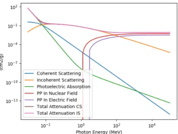
In order to quickly query relative data in nuclear science and particle physics experiments external to standard datasets of constants. A set of application programming interface (API) programs were written into the Grasshopper processing tools such that these databases could be incorporated into the use of Grasshopper. In benchmarking the output of Grasshopper to Geant4, we can look at the output of these databases such as those provided by NIST to prove Grasshopper. The APIs written for grasshopper pull data from these established web databases with an emulator. This emulator creates a web browser which can go and retrieve your work. Grasshopper simulations that are based on the Geant4 toolkit are dependent on a set of libraries and internal data structures provided by CERN. These dependencies such as NDF for capturing constants related to neutron transport are potentially apt to included small errors between empirical constants and the real world. Some of these differences can be accounted for in the evaluation of the differences between Grasshopper based Geant4 simulations and benchmarking data gathered here from trusted empirical databases. Figures 4 and 5 show the use of Grasshopper web APIs to pull XCOM related data and plots.

In addition to evaluating these databases with a Grasshopper API. There is interest in the existing simulation community on a set of standards in particle simulation. Various Monte Carlo methods are commonly used with all trusted tools without a common standard to apply to simulation engines or models. These models are used by the prominent MCNP and OpenMC tools.

3.3.3 Developing Grasshopper Simulation Automation Tools

An essential component of experimentation is repeatability. The test–retest reliability of a simulation is defined as the closeness of the agreement between the results of successive simulations carried out under the same input conditions. In other words, the measurements are taken by a single person or instrument on the same item is that

Figure 4: Helium transport cross sections pulled via API from XCOM database.

Figure 5: Iron transport cross sections pulled via API from XCOM database.

the results between two GDML files intended to Grasshopper simulations prepared directly in the GDML input file passed to Geant4 are not standardized between users.

In order to ensure repeatability for the simulations and tools presented in this thesis, all data files are presented and hosted on the GitHub repository for Grasshopper in a separate section.

3.4

Benchmarking Methods

The simulations generated for the thesis were analyzed with post-processing scripts written for the Grasshopper data output. There are three environmental simulation variables to set for a Grasshopper simulation, these are

enumerated below and represent the main output parameters examined with Grasshopper currently.

1. SaveSurfaceHitTrack

2. SaveEdepositedTotalEntry 3. SaveTrackInfo

3.4.1 Benchmarking Figures of Merit

To benchmark the output of the grasshopper, we perform series of simulations involving protons, gammas, and fast and epithermal neutrons in SaveSurfaceHitTrack mode. For protons we use the energy loss as the relevant metric. For neutral particles the total transmission is calculated, and compared to predictions using cross sections [?] and mass attenuation coefficients[?]. For epithermal neutrons we perform additional checks where energy dependent transmission is simulated, and compared with predictions based on ENDF cross sections.

Viewing the comparisons between empirical results and simulated results can provide a sense of how close Geant4 based simulations can achieve reality. Quantitatively, a set of quantities of merit or figures of merit have been chosen for Grasshopper benchmarks.

The primary two figures are the transmission coefficient for uncharged particles and energy loss for charged particles.

The results of the simulations for neutrons and photon attenuation are provided in the Tables 3 and 4, along with comparisons to the transmission calculations using the NNDC and XCOM nuclear databases. The results for photons indicate strong agreements to within <1%. The neutron attenuation simulation results agree to ≤1%, with deviations likely due to the small differences between the nuclear databases.

η = I I0

(14)

The results of simulated energy loss are then compared to calculations of the energy loss in the air using NIST tables. Since dE/dx in the tables is listed as function of energy, an iteration needs to be performed, using the following formula:

E(xj) = E(xj−1) +

dE(E(xj−1))

dx ∆x

where j is the step in the iteration, ∆x is the step size in distance, and dE(E)/dx is the value of the stopping power extracted from the PSTAR table. This then produces a lookup table of the form {xj; Ej}. Last, the table

can be differentiated along xj, producing a table of {xj; dEj/dx}, describing the stopping power’s dependence on

The results of the simulation for 10 MeV protons in air and comparisons to the PSTAR-based calculations can be seen in Figure ??. The plot shows the protons ranging out at the distance of ∼1 m in air. The comparison shows a good agreement between the theoretical and the simulation results, and indicates a correct functioning of the SaveSurfaceHitTrack tracking mode.

3.4.2 Benchmarking Analysis Methods

For transmission or energy loss differences, a greater than 100% difference can often be interpreted as a failure of the simulation to match reality. However, it is important to understand that the quantity of interest becomes a smaller fraction of the overall value is the change is subtle enough. An example of this is characteristic of gamma radiation through air. Gamma radiation loses an incredibly small amount of energy in air for the same thickness travelled as beta or alpha radiation. Similarly, the percent difference for a Grasshopper simulation in evaluating gamma particle transport can be orders of magnitude larger than that for alpha particle transport. Therefore, comparisons between batches of simulations are not as effect as direct comparisons between provided values and simulated values.

3.5

Online Documentation for Grasshopper

Documentation of Grasshopper C++ and Python scripts can be found online (see footer). Providing online resources for learning Grasshopper hopes to show more programmers and physicists how to use the tools shown in this thesis. The documentation is generated using the Sphinx library for Python. The website is hosted through the non-profit, web hosting service readthedocs. This method of providing documentation is shared by the neutron simulation program ’OpenMC’ [8].

1 2

1_{Grasshopper online docs: https://grasshopper.readthedocs.io/en/latest/} 2_{OpenMC online docs: https://docs.openmc.org/en/stable/}

4

Results and Discussion

This section presents the benchmarks of the thesis. These benchmarks are presented by comparisons between Grasshopper produced results and empirical results. The output data file of Grasshopper can be analyzed and compared against a set of datasets produced by national labs. Stopping power and total cross sections for various particles and energies are published on the websites for the general public. This process of benchmarking makes up an important part of the results of this thesis. The benchmarking process compares other simulation processes and performance results to industry and academia tests. Dimensions typically measured in other simulations as compared to Grasshopper are quality of results (coherence), time to run, and computational complexity or ’cost’. The benchmarks provided here will include the following; stopping power, transmission coefficients, and comparisons to data for various particle interactions. From NIST, sampled results from the following databases will be verified; PSTAR, ASTAR, and ESTAR. In addition, the BNL neutron interaction database and NISTs XCOM will be compared against Grasshopper outputs.

The Grasshopper front-end provides a new method of using Geant4 in the physics community for quickly generated simulations. In the results, implementation of a graphical user interface (GUI) or command line interface (CLI) tool are mentioned.

4.1

Benchmarking Against NIST Databases

A set of tables and constants remain indispensable as a means of quickly looking up constants related to particle transport, but there is an need for computer-readable databases that can generate results on stopping power and transmission of radiation. In order to meet the need, a report presented the web databases ESTAR, PSTAR, and ASTAR which calculate stopping powers, ranges and related quantities, for electrons, protons and helium ions. The underlying methods were developed by members of a report committee sponsored by the International Commission on Radiation Units and Measurements (ICRU).

As a default option, ESTAR generates stopping powers and ranges for electrons which are the same as those tabulated in ICRU Report 37 (ICRU, 1984) for a variety of materials at 81 kinetic energies between 10 keV and 1000 MeV. ESTAR can also calculate similar tables for any other element, compound or mixture. It can also calculate stopping powers at any set of kinetic energies between 1 keV and 10 GeV.

For protons and helium ions, PSTAR and ASTAR generate the stopping powers and ranges tabulated in ICRU Report 49 (ICRU, 1993) for materials at 133 kinetic energies between 1 keV and 10 GeV for protons, and 122 kinetic energies between 1 keV and 1 GeV for helium ions. These databases can calculate similar results at any other energy between these limits through interpolation.

For uncharged particles, neutrons and photons are examined. Data for comparison for these particles comes from the Brookhaven National Laboratory website and NISTs XCOM database for neutrons and gammas

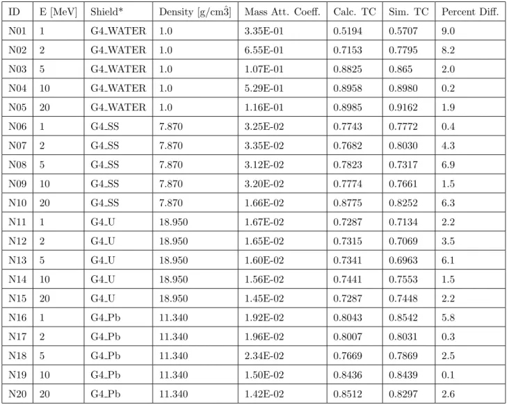
4.1.1 Neutron Benchmarks (BNL/NNDC)

Brookhaven National Lab conducts testing and evaluation of neutron beams on various materials at different energies and angles. The fields of neutron diffraction and neutron imaging have provided a need for crucial databases that describe these processes. Since the results are not straightforwardly analytical, empirical results are desired. Grasshopper can estimate these empirical results through Monte Carlo simulation. A set of 20 simulations were chosen to gauge Grasshoppers ability to estimate constants posted by BNL.

ID E [MeV] Shield* Density [g/cmˆ3] Mass Att. Coeff. Calc. TC Sim. TC Percent Diff.

N01 1 G4 WATER 1.0 3.35E-01 0.5194 0.5707 9.0 N02 2 G4 WATER 1.0 6.55E-01 0.7153 0.7795 8.2 N03 5 G4 WATER 1.0 1.07E-01 0.8825 0.865 2.0 N04 10 G4 WATER 1.0 5.29E-01 0.8958 0.8980 0.2 N05 20 G4 WATER 1.0 1.16E-01 0.8985 0.9162 1.9 N06 1 G4 SS 7.870 3.25E-02 0.7743 0.7772 0.4 N07 2 G4 SS 7.870 3.35E-02 0.7682 0.8030 4.3 N08 5 G4 SS 7.870 3.12E-02 0.7823 0.7317 6.9 N09 10 G4 SS 7.870 3.20E-02 0.7774 0.7661 1.5 N10 20 G4 SS 7.870 1.66E-02 0.8775 0.8252 6.3 N11 1 G4 U 18.950 1.67E-02 0.7287 0.7134 2.2 N12 2 G4 U 18.950 1.65E-02 0.7315 0.7069 3.5 N13 5 G4 U 18.950 1.60E-02 0.7341 0.6963 6.1 N14 10 G4 U 18.950 1.56E-02 0.7441 0.7553 1.5 N15 20 G4 U 18.950 1.45E-02 0.7287 0.7448 2.2 N16 1 G4 Pb 11.340 1.92E-02 0.8043 0.8542 5.8 N17 2 G4 Pb 11.340 1.96E-02 0.8007 0.8031 0.3 N18 5 G4 Pb 11.340 2.34E-02 0.7669 0.7869 2.5 N19 10 G4 Pb 11.340 1.50E-02 0.8436 0.8439 0.1 N20 20 G4 Pb 11.340 1.42E-02 0.8512 0.8297 2.6

Table 3: Grasshopper Neutron Simulations versus Calculations. *The material G4 SS is an alias for G4 STAINLESSSTEEL.

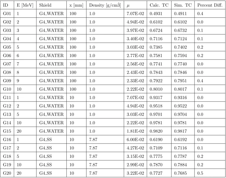
4.1.2 Gamma Benchmarks (Gamma)

The XCOM database from NIST provides lists of mass attenuation coefficients and cross section values. In the benchmarks provided here for gamma particle transport, gradual changes in the transmission coefficient were examined for small variation in energy. It can be seen in the percent differences between benchmarks that the simulation results are consistently accurate to a similar margin for both changes in energy and multiple, common shielding materials. In these simulations, the detector had to be placed much further from the shield material since small scattering angle events occurred at a non-negligible frequency.

ID E [MeV] Shield x [mm] Density [g/cmˆ3] µ Calc. TC Sim. TC Percent Diff. G01 1 G4 WATER 100 1.0 7.07E-02 0.4931 0.4911 0.4 G02 2 G4 WATER 100 1.0 4.94E-02 0.6102 0.6102 0.0 G03 3 G4 WATER 100 1.0 3.97E-02 0.6724 0.6732 0.1 G04 4 G4 WATER 100 1.0 3.40E-02 0.7116 0.7124 0.1 G05 5 G4 WATER 100 1.0 3.03E-02 0.7385 0.7402 0.2 G06 6 G4 WATER 100 1.0 2.77E-02 0.7581 0.7594 0.2 G07 7 G4 WATER 100 1.0 2.56E-02 0.7741 0.7740 0.0 G08 8 G4 WATER 100 1.0 2.43E-02 0.7843 0.7846 0.0 G09 9 G4 WATER 100 1.0 2.33E-02 0.7922 0.7951 0.4 G10 10 G4 WATER 100 1.0 2.22E-02 0.8010 0.8017 0.1 G11 1 G4 WATER 10 1.0 7.07E-02 0.9317 0.9316 0.0 G12 2 G4 WATER 10 1.0 4.94E-02 0.9518 0.9522 0.0 G13 5 G4 WATER 10 1.0 3.03E-02 0.9701 0.9704 0.0 G14 10 G4 WATER 10 1.0 2.22E-02 0.9781 0.9781 0.0 G15 20 G4 WATER 10 1.0 1.81E-02 0.9820 0.9817 0.0 G16 1 G4 SS 10 7.87 6.00E-02 0.6190 0.6192 0.0 G17 2 G4 SS 10 7.87 4.27E-02 0.7109 0.7116 0.1 G18 5 G4 SS 10 7.87 3.15E-02 0.7775 0.7787 0.2 G19 10 G4 SS 10 7.87 2.99E-02 0.7870 0.7884 0.2 G20 20 G4 SS 10 7.87 3.22E-02 0.7727 0.7685 0.5

Table 4: Grasshopper Neutron Simulations versus Calculations. The variable x refers to the thickness of the shielding material. *The material G4 SS is an alias for G4 STAINLESS-STEEL.

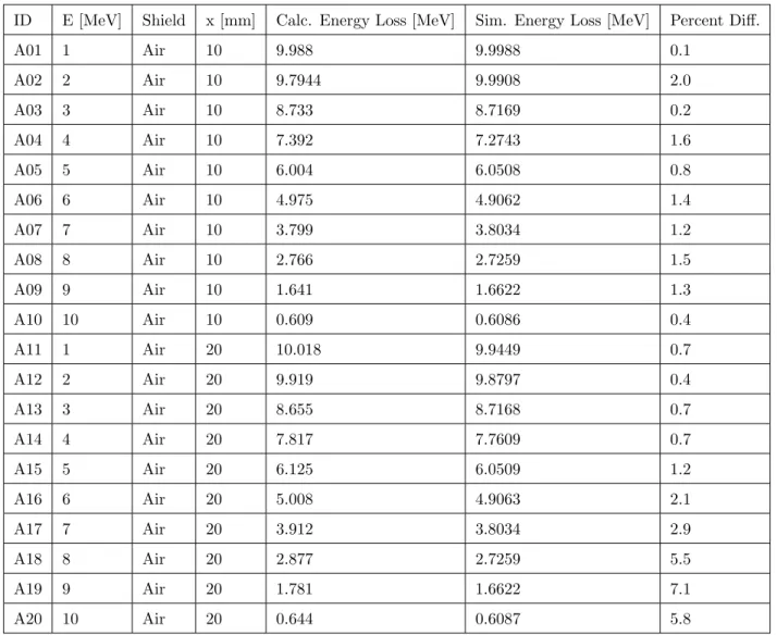
4.1.3 Alpha Benchmarks (ASTAR)

The ASTAR database provides stopping power, CSDA range, radiation yield, and density effect parameters for alpha particle transit through various materials. Alpha particles are much more massive than beta particles and still more than that of protons, as a result, the CSDA range of alpha particles is less than that of either particle.

ID E [MeV] Shield x [mm] Calc. Energy Loss [MeV] Sim. Energy Loss [MeV] Percent Diff.

A01 1 Air 10 9.988 9.9988 0.1 A02 2 Air 10 9.7944 9.9908 2.0 A03 3 Air 10 8.733 8.7169 0.2 A04 4 Air 10 7.392 7.2743 1.6 A05 5 Air 10 6.004 6.0508 0.8 A06 6 Air 10 4.975 4.9062 1.4 A07 7 Air 10 3.799 3.8034 1.2 A08 8 Air 10 2.766 2.7259 1.5 A09 9 Air 10 1.641 1.6622 1.3 A10 10 Air 10 0.609 0.6086 0.4 A11 1 Air 20 10.018 9.9449 0.7 A12 2 Air 20 9.919 9.8797 0.4 A13 3 Air 20 8.655 8.7168 0.7 A14 4 Air 20 7.817 7.7609 0.7 A15 5 Air 20 6.125 6.0509 1.2 A16 6 Air 20 5.008 4.9063 2.1 A17 7 Air 20 3.912 3.8034 2.9 A18 8 Air 20 2.877 2.7259 5.5 A19 9 Air 20 1.781 1.6622 7.1 A20 10 Air 20 0.644 0.6087 5.8

Table 5: Grasshopper alpha simulations versus calculations. Density of air in all simulations is taken as ρ = 0.001kg/m3. The variable x refers to the thickness of the shielding material.

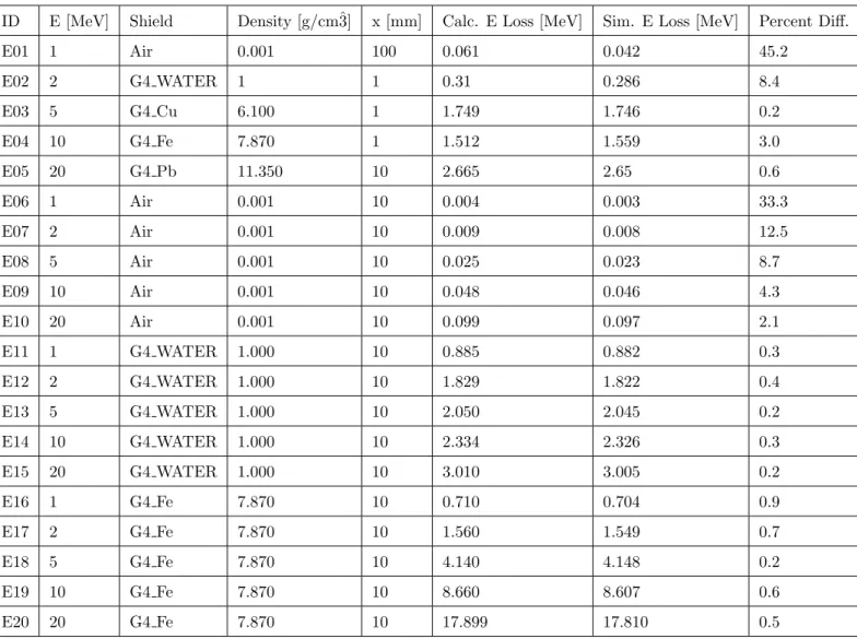
4.1.4 Beta Benchmarks (ESTAR)

Benchmarks chosen for beta particles considered material dependencies on energy loss. For metals, such as copper and iron, the energy loss is very similar and climbs with increases to atomic number. As particle energy increases, the energy decrements are smaller since faster particle spend less time interacting with passing atoms.

ID E [MeV] Shield Density [g/cmˆ3] x [mm] Calc. E Loss [MeV] Sim. E Loss [MeV] Percent Diff.

E01 1 Air 0.001 100 0.061 0.042 45.2 E02 2 G4 WATER 1 1 0.31 0.286 8.4 E03 5 G4 Cu 6.100 1 1.749 1.746 0.2 E04 10 G4 Fe 7.870 1 1.512 1.559 3.0 E05 20 G4 Pb 11.350 10 2.665 2.65 0.6 E06 1 Air 0.001 10 0.004 0.003 33.3 E07 2 Air 0.001 10 0.009 0.008 12.5 E08 5 Air 0.001 10 0.025 0.023 8.7 E09 10 Air 0.001 10 0.048 0.046 4.3 E10 20 Air 0.001 10 0.099 0.097 2.1 E11 1 G4 WATER 1.000 10 0.885 0.882 0.3 E12 2 G4 WATER 1.000 10 1.829 1.822 0.4 E13 5 G4 WATER 1.000 10 2.050 2.045 0.2 E14 10 G4 WATER 1.000 10 2.334 2.326 0.3 E15 20 G4 WATER 1.000 10 3.010 3.005 0.2 E16 1 G4 Fe 7.870 10 0.710 0.704 0.9 E17 2 G4 Fe 7.870 10 1.560 1.549 0.7 E18 5 G4 Fe 7.870 10 4.140 4.148 0.2 E19 10 G4 Fe 7.870 10 8.660 8.607 0.6 E20 20 G4 Fe 7.870 10 17.899 17.810 0.5

Table 6: Grasshopper beta particle simulations versus calculated values. The variable x refers to the thickness of the shielding material.

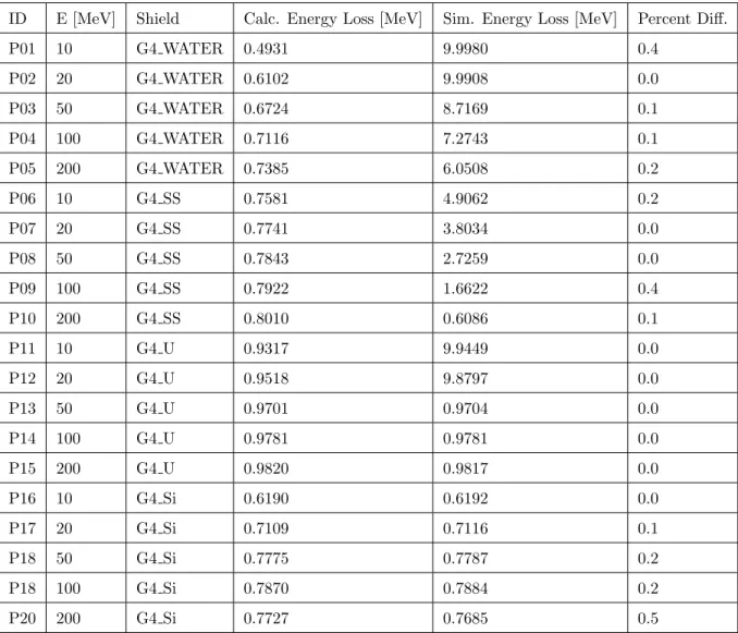
4.1.5 Proton Benchmarks (Protons)

Proton benchmark simulation were chosen to evaluate the energy loss of the ions for a wide range of different atomic number in the shield material. For the case of the water benchmarks, P01 to P05, constants of Z=1 and Z=6 for hydrogen and oxygen respectively are considered by the underlying physics of Geant4 and the formulas used by PSTAR. On the other end of the spectrum in Z, benchmarks P11 to P15 look at

ID E [MeV] Shield Calc. Energy Loss [MeV] Sim. Energy Loss [MeV] Percent Diff.

P01 10 G4 WATER 0.4931 9.9980 0.4 P02 20 G4 WATER 0.6102 9.9908 0.0 P03 50 G4 WATER 0.6724 8.7169 0.1 P04 100 G4 WATER 0.7116 7.2743 0.1 P05 200 G4 WATER 0.7385 6.0508 0.2 P06 10 G4 SS 0.7581 4.9062 0.2 P07 20 G4 SS 0.7741 3.8034 0.0 P08 50 G4 SS 0.7843 2.7259 0.0 P09 100 G4 SS 0.7922 1.6622 0.4 P10 200 G4 SS 0.8010 0.6086 0.1 P11 10 G4 U 0.9317 9.9449 0.0 P12 20 G4 U 0.9518 9.8797 0.0 P13 50 G4 U 0.9701 0.9704 0.0 P14 100 G4 U 0.9781 0.9781 0.0 P15 200 G4 U 0.9820 0.9817 0.0 P16 10 G4 Si 0.6190 0.6192 0.0 P17 20 G4 Si 0.7109 0.7116 0.1 P18 50 G4 Si 0.7775 0.7787 0.2 P18 100 G4 Si 0.7870 0.7884 0.2 P20 200 G4 Si 0.7727 0.7685 0.5

Table 7: Grasshopper proton simulations versus calculations. All simulations use a shield thickness of 1mm. *The material G4 SS is an alias for G4 STAINLESS-STEEL.

4.2

Energy Loss and Bragg Peak Simulation

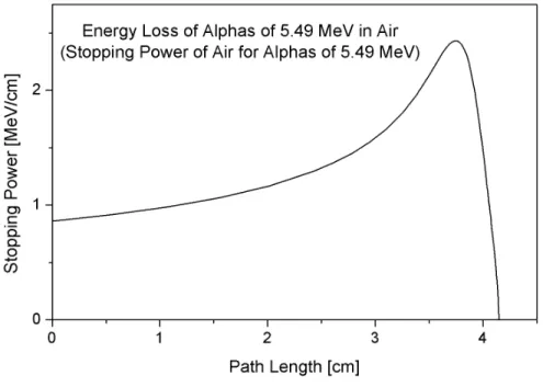
A Bragg curve plots the energy loss of ionizing radiation during its travel through matter. A Bragg peak is a pronounced peak on the Bragg curve briefly before charged particles deposit all significant energy in transit. For protons, α-rays, and β-rays, the peak occurs immediately before the particles come to rest. A set of simulations

to compare simulated Bragg peaks against theoretical calculations based on given databases was carried out. An example of a Bragg curve for alpha particles is given in figure 6.

Figure 6: Example of the calculated Bragg peak for alpha particles.

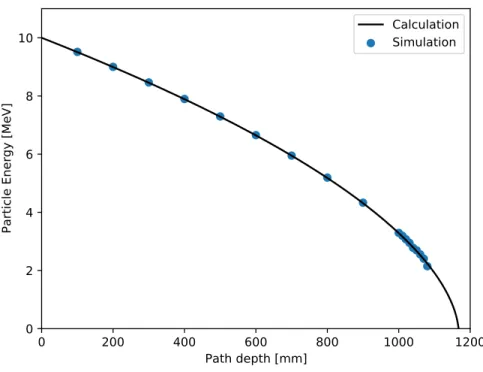
For the generation of calculated results using PSTAR, an iterative approach was used where the energy decrement was a re-evaluated function of the energy dependent stopping power. Figure 7 shows the strong agreement between the Grasshopper simulated energy and calculated energy for different lengths into air for an incident beam of 10 MeV protons.

An example of a figure used to determine the placement of a proton beam for use in medical therapy. Note the position of the peak at different depths into tissue. The native proton beam refers to a monoenergetic beam. The modified proton beam slows a fraction of a monoenergetic beam such that the normalized ’dose’ or energy deposition is constant over a length of tissue, this is used in the therapy of cancerous tumors.

0

200

400

600

800

1000

1200

Path depth [mm]

0

2

4

6

8

10

Particle Energy [MeV]

Calculation

Simulation

Figure 7: Full energy loss of protons through air measured in simulation versus calculations.

Figure 8: Standard and modified Bragg peaks for proton beams and a comparison energy deposition by a photon beam.

4.3

Features in the Grasshopper CLI

Grasshopper can be used from a standard terminal interface. The program has been operated as a terminal command supplied two files as the arguments. Now, a command line interface (CLI) is available to use Grasshopper. The CLI can be used to evaluate GDML input files, generate new input files, run batches of simulations, and analyze results. Additionally, a set of APIs used to pull data from NIST databases is included in other tools written for

the benchmarks provided in this thesis.

4.4

Features for a Grasshopper API

The core functionality of Grasshopper is its method of performing a simulation as a subprocess. This software can run in the background of a computer serving other programs. For example, if a website wanted to offer a simulation service, Grasshopper could run in the background as an application programming interface (API). An API has been built for Grasshopper in addition to the CLI.

4.5

Grasshopper Simulation Automation Tools

The CLI tool allows for the simultaneous and sequential operation of multiple Grasshopper simulations. In evaluat-ing a particular experiment or radiation event, there may be an interest in multiple geometries or energy levels. In these cases, the simulation automation scripts included in the CLI offers a Grasshopper user the ability to launch as many simulations as they would like. In a multi-core computational system, this may involve either starting multiple instances of Grasshopper at once or running on instance as fast as possible.

5

Application of Grasshopper

5.1

Range of Viable Simulation in Grasshopper

Discoveries of the validation, processing, and benchmarking results in more details bringing up inherent operations of Geant4 which relate to real world processes. Underlying Geant4 frameworks limit the range of energies that a particular particle is tracked. As a result, simulations in Grasshopper can only evaluate particle transmission and energy loss at levels typically encountered in radiative energy physics.

Quantity Range Note

Target Z 1 < Z < 94 Atomic number Particle E 1 < E < 100 MeV of incident beam Target Thickness 1 < x < 100 millimeters

Table 8: Grasshopper simulation range of variables tested in this thesis.

5.2

Grasshopper Sources of Error

Monte Carlo simulations are prone to errors regarding small and large step sizes. The step has two points and also a delta for a particle (energy loss on the step, time-of-flight spent by the step, etc.). Cutoffs are another source of error, since Geant4 does not attempt to simulation incredibly low energy interactions of individual electrons forming bonds with the medium they lose energy, there is a lack of tracking for particles once they reach a ”cut off”. Another form of error can arise from an improper position of geometries in the GDML input file. Grasshopper uses Geant4 through the GDML parser object. This path to using Geant4 is limited by the features built by the CERN developers writing Geant4.

The C++ methods developed in Geant4 which operate the core functionality of particle transport used by Grasshopper use finite difference methods. Finite difference methods can suffer from frequency shifts in data sources. As a function is evaluated, if local minimum or maximum are used to determine results, then averages can be reported incorrectly. Some documentation problems exist for Grasshopper regarding the methods used in Geant4 back-end. When running > 16 MeV neutrons the code will slow down to a point of stopping. The code is optimized to run in two configurations: ”SurfaceHit” analysis, which provides energy, position, and momentum information on the flux of particles through a ”detector” surface. It will generate multiple entries for multiple tracks crossing a surface for a single MC event. However, if one of the tracks then backscatters and crosses the surface again it will be ignored. Secondly, ”EnergyDeposited” analysis, providing deposited energy results for every event.

5.3

Future Work to be Considered

The tools presented in this thesis allow for quicker use of Grasshopper and Geant4 simulations. Through enabling a quicker method of generating and evaluating simulations, future work into iterative studies is possible [1]. Addition-ally, improving the CLI tool for generating and running simulations will speed up the process of using Grasshopper. This can be accomplished through a collaborative project between multiple Grasshopper users with experience in Python or C++ programming. The CLI currently has limited functionality in generating Grasshopper input files. The GDML files created by the CLI can only vary a subset of the full set of available features in the GDML. Additional software construction could benefit experimenters who seek to conduct experiments beyond the nature of the benchmarks presented in this thesis with the Grasshopper CLI or API tools.

6

Conclusions

The benchmarking of Grasshopper against known values gives confidence in using Grasshopper as a Geant4 level simulation tool in the computational physics community. In this thesis, a set of tables and figures show the relationship between a wide range of simulated conditions and known nuclear constants. By allowing users of Geant4 an easier method of generating simulations, the time it takes to develop an insight is drastically reduced. The tables presented in the results section demonstrate a proven range of variables for use in Grasshopper based simulations. The open source nature of the Geant4 simulation software allows for easy use and collaboration. This thesis and associated online documentation discusses the software’s construction such that it may be easily be picked up by a wider audience of engineers and scientists.

Through developing methods for continuous development and integration of Grasshopper software, the software will be able to follow the future development of Geant4. Another goal beyond continuous development and integration of Grasshopper are contributions to the codebase into the Debian standard repositories. Contributing to the standard repositories would bring Grasshopper more recognition and make it easier to download and install. By improving and better framing the Grasshopper simulation engine, particle simulation scientists and engineers can have greater confidence in their results before and after conducting an experiment.

In this thesis, Grasshopper is presented and benchmarks are provided. This software tool is a Geant4 front-end that allows for rapid modeling of small experiments consisting of a few detectors. The software inputs and outputs have been described, along with the basic logic behind some of its tracking and tallying algorithms. Furthermore, validation, and benchmarking results have been provided, showing that Grasshopper correctly models energy loss by MeV charged particles, transmission attenuation by MeV photons and MeV and eV neutrons.

References

[1] S. A. et al., “Geant4—a simulation toolkit,” Nuclear Instruments and Methods in Physics Research Section A: Accelerators, Spectrometers, Detectors and Associated Equipment, vol. 506, no. 3, p. 250, 2003.

[2] J. A. et al., “Recent developments in geant4,” Nuclear Instruments and Methods in Physics Research Section A: Accelerators, Spectrometers, Detectors and Associated Equipment, vol. 835, no. 1, p. 186, 2016.

[3] A. DANAGOULIAN, “Grasshopper,” 2020.

[4] E. Mendoza, D. Cano-Ott, T. Koi, and C. Guerrero, “New standard evaluated neutron cross section libraries for the geant4 code and first verification,” IEEE Transactions on Nuclear Science, vol. 61, no. 4, pp. 2357–2364, 2014.

[5] S. YIP, Nuclear Radiation Interactions. World Scientific, MIT, 2014.

[6] J. R. Taylor, An Introduction to Error Analysis. Wiley Professional, 1976.

[7] G. F. Knoll, Radiation Detection and Measurement 3rd Edition. John Wiley and Sons, Inc., 1999.

[8] e. a. Paul K. Romano, “Open mc,” 2020.

[9] NIST, “Stopping-power range tables for electrons, protons, and helium ions,” 2017.

Acknowledgements

The author is very thankful for the help and support of Professor Areg Danagoulian. Without this support, this thesis would have been much less productive. Additionally, readers provided valuable feedback during the writing process and the department of Nuclear Science and Engineering at MIT for their support and encouragement. This thesis work was completed during a time of intense hardship on many individuals involved during the COVID-19 pandemic.