Dynamics of North Atlantic western boundary currents

(1)

DYNAMICS OF NORTH ATLANTIC

WESTERN BOUNDARY CURRENTS

by

Isabela Astiz Le Bras

B.A., University of California, Berkeley (2010)

Submitted in partial fulfillment of the requirements for the degree of Doctor of Philosophy

at the

MASSACHUSETTS INSTITUTE OF TECHNOLOGY and the

WOODS HOLE OCEANOGRAPHIC INSTITUTION February 2017 MASSACHUSE5S TITUTE OF TECHNOLOGY

FEB 222017

LIBRARIES

@2017

The author hereby grants to MIT and WHOI permission to reproduce and to distribute publicly paper and electronic copies of this thesis document in whole or in

part in any medium now known or hereafter created.

A uthor ...

Certified by...

Sign

SI

Accepted by...

Signature redacted

Joint Program in Physical Oceanography

Massachusetts Institute of Technology & Woods Hole Oceanographic Institution Decpnber 23, 2016

ature redacted

John M. Toole Senior Scientist in Physical Oceanography Woods Hole Oceanographic Institution

A Thesis Supervisor

ignature

redacted-Lawrence J. Pratt Chair, Joint Committee for Physical Oceanography Massachusetts Institute of Technology Woods Hole Oceanographic Institution

(2)

(3)

DYNAMICS OF NORTH ATLANTIC WESTERN BOUNDARY CURRENTS

by

Isabela Astiz Le Bras

Submitted to the MIT-WHOI Joint Program in Physical Oceanography on December 23, 2016, in partial fulfillment of the requirements for the degree of Doctor of Philosophy in Physical

Oceanography

ABSTRACT

The Gulf Stream and Deep Western Boundary Current (DWBC) shape the distribution of heat and carbon in the North Atlantic, with consequences for global climate. This thesis employs a combination of theory, observations and models to probe the dynamics of these two western boundary currents.

First, to diagnose the dynamical balance of the Gulf Stream, a depth-averaged vortic-ity budget framework is developed. This framework is applied to observations and a state estimate in the subtropical North Atlantic. Budget terms indicate a primary balance of vor-ticity between wind stress forcing and dissipation, and that the Gulf Stream has a significant inertial component.

The next chapter weighs in on an ongoing debate over how the deep ocean is filled with water from high latitude sources. Measurements of the DWBC at Line W, on the conti-nental slope southeast of New England, reveal water mass changes that are consistent with changes in the Labrador Sea, one of the sources of deep water thousands of kilometers up-stream. Coherent patterns of change are also found along the path of the DWBC. These changes are consistent with an advective-diffusive model, which is used to quantify transit time distributions between the Labrador Sea and Line W. Advection and stirring are both found to play leading order roles in the propagation of water mass anomalies in the DWBC. The final study brings the two currents together in a quasi-geostrophic process model, focusing on the interaction between the Gulf Stream's northern recirculation gyre and the continental slope along which the DWBC travels. We demonstrate that the continental slope restricts the extent of the recirculation gyre and alters its forcing mechanisms. The recirculation gyre can also merge with the DWBC at depth, and its adjustment is associated with eddy fluxes that stir the DWBC with the interior.

This thesis provides a quantitative description of the structure of the overturning circu-lation in the western North Atlantic, which is an important step towards understanding its role in the climate system.

Thesis Supervisor: John M. Toole

Title: Senior Scientist in Physical Oceanography Woods Hole Oceanographic Institution

(4)

(5)

ACKNOWLEDGMENTS

First and foremost, I thank my advisor, John Toole. John gave me the freedom to explore my own ideas, guided me with his thought-provoking questions, and was always available for discussions. I strive to emulate John's careful and creative approach to science as well as his kindness. I am ever thankful for the support and faith he showed me throughout my thesis and look forward to our continued collaborations.

My committee was a great help and a pleasure to interact with. I thank Amy Bower for

many exciting conversations about the North Atlantic, and for reminding me to keep my language precise. Glenn Flierl offered many deep insights as my work developed, and his dedication to science and students is inspiring. Steve Jayne provided invaluable assistance with the QG model he started writing as a WHOI Summer Student Fellow, and found time to meet and help me keep perspective, even during hurricane season. Mike Spall's thoughtful questions and suggestions have shaped this thesis and helped me learn to identify interesting and tractable scientific problems. Finally, I thank Young-Oh Kwon for chairing my defense, for access to his computer server and his enthusiastic teaching.

The WHOI PO department and MIT EAPS departments provided stimulating research environments over the last 5 years. Magdalena Andres and Jake Gebbie have been excellent mentors and I have benefitted enormously from conversations and classes with Joe Pedlosky, Ken Brink, Amala Mahadevan, Terry Joyce, Susan Lozier, Stephanie Waterman, and John Marshall. Thanks are also due to Patrick Heimbach, Chris Hill and Diana Lees Spiegel for providing the ECCO state estimate fields analyzed in Chapter 2.

I am grateful for the opportunities I had to go to sea with John Toole, Ruth Curry, Magdalena Andres, and Leah Trafford. The Line W observations presented in Chapter 3 are the result of many years of hard work by many people, including Michael McCartney, Terry Joyce, Dan Torres, Scott Worrilow, Brian Hogue, the WHOI mooring group, and the crews of the Knorr and Oceanus.

I was also fortunate enough to visit England and Germany over the course of my Ph.D.

and form connections with scientists at Southhampton, Kiel, Hamburg and Bremen. In particular, I thank Martin Visbeck, Jirgen Fischer and Patricia Handmann for hosting my visit to Kiel. I thank Igor Yashayaev for providing the Labrador Sea data used in Chapter

3, and many interesting email conversations.

I have had a lot of fun in the Joint Program. My PO peers, Becca Jackson, Joern Callies,

Alec Bogdanoff and Deepak Cherian provided many interesting scientific discussions, laughs and support. My roommates, Julie van der Hoop and Sophie Chu were like sisters to me, and the many other houses of friends in Woods Hole, at Hinckley, Fern, and Huettner, as well as the far reaches of Falmouth and Cambridge made the long winters full of potluck-fun.

(6)

I also wish to thank Harriet for her love and encouragement, and for making Figure 4-10. I

look forward to many years full of science, cooking and windsurfing together.

Finally, I thank my family. In particular, I thank my brothers and my parents, Luciana Astiz and Ronan Le Bras, for their tireless support and for inspiring me to pursue a career in science. Gracias mama and merci papa!

My research was funded by National Science Foundation grants 0241354, OCE-0726720 and OCE-1332667 as well as a graduate fellowship from the American

Meteoro-logical Society. Support for travel and educational supplies was also provided by the MIT Houghton Fund and the WHOI Academic Programs Office. Special thanks are due to APO and administrators at MIT and the WHOI PO department for running the Joint Program seemlessly.

(7)

LIST OF FIGURES

1-1 Chart of the Gulf Stream by Benjamin Franklin. . . . 17

1-2 Oxygen concentrations from 2000-3000 m measured on the 1925-1927 Meteor cru ise . . . . 18

1-3 A schematic of Atlantic circulation from Stommel (1957). . . . . 19

2-1 Map of WOCE/CLIVAR A22 cruise tracks and the ECCO boundary. . . . 32 2-2 Depth of the study volume in the Gouretski and Koltermann (2004)

clima-tology and ECCO state estimate. . . . . 34

2-3 Average wind stress in the regions of interest from four different products. . . 41

2-4 Time series of wind stress forcing term from satellite data products . . . 43

2-5 Time series of the wind stress forcing and vorticity flux terms in the ECCO m o d el. . . . 44

2-6 Components of calculation of vorticity flux across the A22 cruise track . . . . 48

2-7 As in Figure 2-6 for the ECCO state estimate analysis. . . . . 52 2-8 Time series of the remaining significant terms in the vorticity budget and

demonstration of approximate balance in the ECCO model. . . . . 53 2-9 Maps showing the relationship of f/h contours, time mean depth-averaged

flow and lateral friction for the study volume in the ECCO model. . . . 57

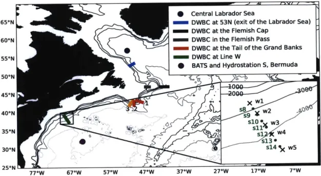
3-1 Map of dataset locations along the path of the Deep Western Boundary Current 64

3-2 Time evolution of a) potential temperature and b) salinity profiles in the central Labrador Sea. . . . . 66 3-3 Map of the Labrador Sea highlighting observation locations used to form the

annual average central Labrador Sea profiles. . . . . 70

3-4 0-S properties in the central Labrador Sea, at Line W moorings and at BATS. 71

3-5 Evolution of 0-S properties at Line W moored array from 2005 to 2013. . . . 73

3-6 Water mass property anomaly time series and mean profiles in the central Labrador Sea and at Line W in neutral density space. . . . . 76 3-7 Results from lagged correlation analysis between Labrador Sea and Line W

layer thickness, potential temperature and salinity anomalies within neutral density bins. . . . . 79 3-8 Mean salinity within water masses for datasets along the path of the DWBC. 82 3-9 Mean salinity within water masses measured by Line W moorings. . . . 83

(10)

3-10 As in Figure 3-8 but for water mass layer thickness. . . . . 85 3-11 As in Figure 3-9 but water mass layer thickness as measured by Line W

m oorings. . . . . 86 3-12 Transit time distributions and sample sinusoidal signals for different limits of

the Waugh and Hall (2005) model. . . . . 91 3-13 Sinusoidal fits to central Labrador Sea and Line W mean dLSW and NEADW

potential temperature, salinity and layer thickness. . . . . 92

3-14 Parameter range of sinusoidal fits to Labrador Sea and Line W potential temperature and salinity data shown in relative amplitude and phase lag space. 93

3-15 Solutions to parameter space sensitivity analysis. . . . 96 3-16 Range of potential transit time distributions solutions from the Labrador Sea

to Line W for dLSW . . . 97

3-17 Normalized cost functions for forward model fits to Line W dLSW potential

temperature, salinity and layer thickness time series. . . . 99

3-18 Best fits from forward model to Line W dLSW potential temperature, salinity

and layer thickness anomaly times series. . . . 100 4-1 Schematic of the barotropic circulation in the western North Atlantic from

Zhang and Vallis (2007), adapted from Hogg (1992). . . . 110

4-2 Meridional structure of the streamfunction, velocity, potential vorticity and meridional potential vorticity gradient at the model western boundary. . . . . 114 4-3 Mean streamfunction (V;) and PV (q) in the upper and lower layers for the

basic m odel setup. . . . 115

4-4 Steepness of bathymetry along the continental slope, and comparison of Line W and model bathymetry and steepness. . . . 118 4-5 Normalized meridional PV gradients and meridional eddy PV fluxes for

av-erages in sections of the recirculation gyre depicted in Figure 4-3. . . . 120 4-6 Time-mean profiles of lower layer PV, 42, relative vorticity, 2, thickness,

(01 - V)2)/S2, and zonal velocity, V2, at the zonal position of jet stabilization,

Xm ..-... ... ... . ... 122. . . .

4-7 Analytic recirculation gyre meridional extent prediction plotted against mea-sured meridional extent in the QG model (both in km) for model configura-tions with different inflowing jet velocities. . . . 123 4-8 Time-mean zonal velocity profiles in the upper model layer at the zonal

po-sition of jet stabilization. . . . 124 4-9 Profiles of meridional eddy PV flux integrated zonally across the recirculation

gyre for model configurations without a slope or DWBC (blue), with a slope, but no DWBC (green), and with both a slope and DWBC (red) . . . 125

4-10 Schematic illustration of the system PV budget in the model lower layer. . . .126 10

(11)

4-11 Cumulative eddy and mean PV flux convergences in the lower layer, integrated northward from the jet axis, y3 . . . 127

4-12 PV budget synthesis for model configurations without a slope or DWBC, with a slope, but no DWBC, and both a slope and DWBC. . . . 128 4-13 The time mean streamfunction in the lower layer, 'i, for model configurations

with varying initial jet strength and proximity to bathymetric slope. . . . 132 4-14 Lower layer meridional eddy PV fluxes integrated zonally along the jet axis

for model configurations shown in Figure 4-13, with an explanatory schematic. 133 4-15 Upper layer PV (qi) snapshots for the model configurations shown in Figures

4-13 and 4-14... ... 135

4-16 Growth rate as a function of zonal wavenumber for the model configurations shown in Figures 4-13 - 4-15 for the inflowing jet profile, and the time mean profiles at 1000 and 1600 km downstream. . . . 136 4-17 As in Figure 4-6, for the model configurations with varying inflowing jet

velocities, and hence jet instability. . . . 137 4-18 Analytic meridional extent prediction against meridional extent in the QG

model (both in km) for model configurations with varying jet velocities, with a slope and DW BC. . . . 138

4-19 PV budget synthesis for model configurations with varying inflowing jet ve-locities, and hence jet instability. . . . 138 4-20 Recirculation gyre and DWBC transports for model configurations with

vary-ing inflowvary-ing jet velocities, and hence jet instability. . . . 139

4-21 As in Figure 4-6, for model configurations with different distances between the unstable jet and DWBC. . . . 141

4-22 PV budget synthesis for model configurations with different distances between the unstable jet and DWBC. . . . 142

4-23 Recirculation gyre and DWBC transports for model configurations with dif-ferent distances between the unstable jet and DWBC. . . . 143

4-24 Nondimensional value of sponge region linear friction coefficient, Rsponge in the m odel dom ain. . . . 147 4-25 Mean lower layer streamfunction, ~2, for different values of the viscosity

co-efficient, A . . . 149 4-26 Meridional profiles of integrate meridional eddy PV flux, and time series of

domain integrated enstrophy and psi variance for model runs in which a slope and DWBC are added sequentially. . . . 151 4-27 As in Figure 4-26, but for model configurations with different inflowing jet

(12)

4-28 Time series of domain integrated enstrophy and 0 for model configurations with inflowing jet velocity of 0.63 m s-1 and 1.44 m s ... . . . 153

4-29 As in Figure 4-26, but for model configurations with different distances be-tween the jet and the center of the bathymetric slope. . . . 154

4-30 Estimates of

f

f(dq2

/dt)dA

during three different time periods, for base case

runs in which a slope and DWBC are added sequentially. . . . 155 4-31 As in Figure 4-30 but for model configurations with different inflowing jet

velocities. . . . 156 4-32 As in Figure 4-30 but for model configurations with different distances

be-tween the jet and the center of the bathymetric slope. . . . 156

(13)

LIST OF TABLES

2-1 Summary of wind stress forcing and advective vorticity flux budget terms in both observations and in the ECCO state estimate. . . . 46 2-2 Summary of all time-mean vorticity budget terms in the ECCO state estimate

and their mean/eddy breakdown. . . . 56

3-1 W ater mass definitions . . . 67

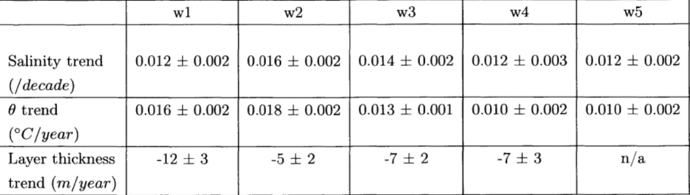
3-2 Trends in dLSW water mass properties measured by Line W moorings. . . . . 87

3-3 Parameters of sinuisoidal fits to mean dLSW properties and resulting solutions. 90 3-4 As in table 3-3 but for NEADW. . . . 94

(14)

(15)

CHAPTER 1

(16)

In the North Atlantic, two large-scale ocean circulation patterns redistribute heat, salt and carbon, with significant consequences for marine ecosystems (Schmittner, 2005), global sea level (Vellinga and Wood, 2008) and climate (Wunsch, 2005; Kwon et al., 2010): the wind-driven and overturning circulations. The wind-wind-driven circulation is forced by the prevailing global wind belts, the easterlies, westerlies and trade winds, forming a subtropical and subpolar gyre in the North Atlantic, each thousands of kilometers wide. The overturning circulation in the North Atlantic is composed primarily of cold water which sinks at high northern latitudes and travels toward the other pole at depth over tens of thousands of kilometers, and a warmer return flow at the surface.

Both of these circulation patterns include relatively strong and narrow (0 100km) cur-rents confined to the basin's western boundary, termed western boundary curcur-rents. This thesis is focused on the western boundary current of the North Atlantic subtropical gyre, the Gulf Stream, and the western boundary current of the North Atlantic overturning cir-culation, the Deep Western Boundary Current (DWBC).

Using a combination of observations and models, in this thesis I investigate the dynamics of the forcing of the Gulf Stream, the propagation of water mass properties in the DWBC and the interaction between the two currents. In this chapter, I will provide background and motivation to contextualize this thesis, as well as a road map for the remaining thesis chapters.

1.1 Historical background

Because of its significant impact on navigation in the western North Atlantic, seafarers have had a sense of the Gulf Stream since the 16th century (MacLeish, 1989). It was famously charted by Benjamin Franklin, who acknowledges whaling Captain Folger for informing him of the course, strength and extent of the stream (see Figure 1-1).

The deep ocean circulation was more elusive. In an essay at turn of the 19th century, Rumford (1800), showed an early appreciation for the high-latitude source of the cold water below the thermocline throughout the world ocean. Yet, as Deacon (1954) wrote, "We have known for 150 years that there is water, nearly ice-cold, at the bottom of the tropical Atlantic Ocean, and that it must flow there from the Antarctic, but we can still argue whether it took 18 years or 1800, and there is as much uncertainty about the forces which move it there." With the Meteor Expedition, from 1925 to 1927, came the first indication that the equatorward spreading of high-latitude water was western intensified. As shown in Figure 1-2, they measured a core of high oxygen water on the west of the Atlantic basin at 2000-3000 m depth (Wiist, 1935).

The basic mathematical theory governing both of these large-scale circulation patterns was proposed by Henry Stommel in the 1940's and 50's (Stommel, 1948; Stommel et al.,

(17)

I AI #I Ii Aar

Figure 1-1: Chart of the Gulf Stream by Benjamin Franklin. Appeared in Transactions of the American Philosophical Society, 1786. Image courtesy of the Library of Congress, mounted on cloth.

1958). Our basic understanding of the circulation in the North Atlantic continues to be shaped by his insights, and his schematic of the superposition of the wind-driven and over-turning circulations in Atlantic, Figure 1-3, remains relevant to our current understanding

of the large-scale Atlantic circulation (Richardson, 2008). At the heart of both of these

theories is the significance of planetary rotation on the large-scale movement of fluids, which can be conveniently framed in terms of Potential Vorticity (PV).

(18)

AO 600 4O 200 Of 210

11/0

f4 800 WO 400 200 00 200 40*

M Lana' ais 0 -IMZM -+ "1ptaus'rqtg 6 -- AZbwI9onen

Figure 1-2: Oxygen concentrations from 2000-3000 m measured on the Image from Richardson (2008).

1925-1927 Meteor cruise. 18 40, 404 I nu I I 4--3M

(19)

aE

Figure 1-3: A schematic of Atlantic circulation from Stommel (1957). His caption: A schematic interpretation of the circulation in the Atlantic Ocean constructed by superposition of an internal model associated with flow across a level surface L at mid-depth (a) and a purely wind-driven circulation in the surface layers (b). The sum of these two is shown in figure (c).

(20)

1.2 Potential Vorticity (PV)

PV is a quantity with enormous utility in physical oceanography. It is a scalar field that emerges when the momentum and buoyancy equations are combined and sheds light on the essential forcing mechanisms that control the circulation. Because it features in each of the main thesis chapters, in this section I will describe its derivation and highlight the different forms of PV that will appear throughout.

The dynamics considered in this thesis are in the low Rossby number limit. The Rossby number describes the relative magnitude of advective and Coriolis terms in the momentum equation and hence the importance of rotation. The Rossby number is

Ro = U (1.1)

fL'

where U is a characteristic velocity scale, L a characteristic length scale and

f

is the Coriolis parameter, which is twice the frequency of the earth's rotation multiplied by the sine of the latitude, to project the vector of the earth's rotation onto the vertical direction of the local coordinate frame. A low Rossby number means that the frequency of the described motions is smaller than the frequency of rotation in the local coordinate frame, which can mean that the described motions are slow or occur over large scales. In general, this corresponds to motions in the mid- and high-latitude ocean that occur over time scales longer than weeks and spatial scales larger than hundreds of kilometers.

In the low Rossby number limit, the primary balance of horizontal momentum reduces to the geostrophic balance:

f

xu = V, (1.2)

P0

where u is the horizontal velocity vector, p is pressure, po is a reference density and cross products and gradients are in the horizontal plane. In geostrophic balance, flow follows contours of pressure. This principle enables the use of sea surface height to infer flow patterns, for example.

By taking the curl of the horizontal momentum equations to form a vorticity equation,

this first order steady state balance is eliminated, as the curl of a gradient is zero. This draws the smaller terms in the momentum equation to the forefront, such as forcing and dissipation. Though the dominant balance can be eliminated through the vorticity equation to gain insight into forcing mechanisms, it can be difficult to interpret the vorticity equation as it describes a vector field. To overcome this, the vorticity equation can be spatially integrated to form an equation for a scalar field, the circulation. In Chapter 2, we construct a circulation equation and diagnose the size of its terms to gain insight into the large-scale vorticity balance of the Gulf Stream.

(21)

However, the terms in a circulation equation depend on the integration volume. The PV equation, which emerges from the combination of the momentum and buoyancy equations, is more general because it describes a full scalar field. Holland et al. (1984) summed up the power of PV effectively in their statement, "A theory of the scalar fields q (PV) and p (density) is tantamount to a theory of the general circulation."

The most general form of PV is due to Ertel (1942),

q= 2M + oVp, (1.3)

p

where Q is the earth's rotation vector and w = V x u is the vorticity of the flow, referred to as the relative vorticity; where V, u and w are all 3-D vectors. Ertel's PV does not require a small Rossby number, but it does require that p be conserved. The conservation equation for PV is

-- + u - Vq = F, (1.4)

Ot

so that PV is conserved following the flow, barring forcing or dissipation, F.

In this thesis we focus on the shallow water limit, in which horizontal length scales are much larger than vertical length scales, so that vertical gradients dominate. This limit is relevant to this thesis as we focus on phenomena with large spatial scales 0(100 km) relative to the depth of the ocean (a 5 km). We further assume that the ocean is in hydrostatic balance and that isopycnals are material surfaces, so that PV reduces to

f+ &p _f

(

p + h (1.5)

p Oz h

where h is the vertical distance between isopycnal surfaces, and = -

g,

is the vertical

component of the relative vorticity. In Chapter 3, we further approximate PV by h, and use changes in layer thickness between isopycnals to diagnose changes in PV.

The model used in Chapter 4 is in the quasi-geostrophic limit, in which the flow is assumed to be nearly in geostrophic balance, and perturbations in layer depth are much smaller than the total water depth. The small departures from geostrophy allow the system to evolve in time. Quasi-Geostrophic PV (QGPV) can be approximated from shallow-water

PV, as shown in Vallis (2006):

f_ +( 1 1

, -- (f +()(1 - h'/H) ~ -(fo + Oy + - foh'/H), (1.6)

H(1 + h'/H) H H

where H is the mean depth of a layer with constant density, h' denotes deviations from this mean, fo is the mean Coriolis parameter and / is the linearized Coriolis gradient. In this approximation we have used that h'/H < 1, and only kept terms that are O(foRo) or

(22)

larger. Since fo/H is a constant, the QGPV is commonly defined as

QGPV =,3y+ ( - foh'/H. (1.7)

QGPV

is conserved along geostrophic flow contours absent forcing or dissipation, and is a linear function of the geostrophic streamfunction, so that QGPV can be inverted to deter-mine the flow. The quasi-geostrophic framework facilitates the interpretation of dynamics in terms of PV, and because of their simplicity they were the first equations used to model the effects of eddies on the mean circulation (Holland, 1978). In Chapter 4, we use the two-layer

QGPV equations to study the effects of the circulation driven by Gulf Stream eddies on the

DWBC.

The essence of western boundary current theory can be explained through the conser-vation of PV. The conserconser-vation of PV implies that flow cannot cross contours of

f,

or lines of latitude, without a compensating change in another component of PV, or the action of forcing or dissipation. In western boundary current theory, changes in

f

are allowed by dissipation of PV from friction in the western boundary current. For example, the Gulf Stream's northward motion, and hence increasing

f

is delivered by the positive PV (vortic-ity) associated with friction acting to counter the Gulf Stream. Importantly, the PV injected

by friction on the western boundary is the correct sign to balance change in planetary PV

associated with meridional motion regardless of the direction of the current or hemisphere. Indeed, western boundary currents are observed in each ocean basin in each hemisphere.

1.3 Scientific context

The wind-driven circulation

In Stommel's theory for the wind-driven circulation, the wind forcing over the ocean basin is dissipated in an intense western boundary current by bottom friction. Stommel (1948)'s theory and its extension by Munk (1950), were so successful because of their simplicity and ability to reproduce the main features of the circulation, but they underestimated the Gulf Stream's transport. Both theories also assumed a homogeneous ocean with flat bathymetry, in order to make the problem tractable.

Several theoretical developments addressed these limitations. Fofonoff (1954) showed that inertial basin modes can arise when the nonlinear advective term is included, without bounds on the magnitude of transport. Holland (1972) suggested that adding stratification and bathymetry would correct the Gulf Stream transport. Finally, Holland and Rhines

(1980) demonstrated that eddies could force recirculations about an unstable jet, which can

also contribute to the transport of the Gulf Stream.

There is an appreciation for all of these developments in the recent literature, and

(23)

vances in modeling the ocean have enabled the detailed diagnosis of PV transformations in ocean models (Czaja and Hausmann, 2009; Deremble et al., 2014; Yeager, 2015; Schoonover et al., 2015). However, the connection between the classical balances of Stommel and Munk and the detailed PV maps in ocean models is not straightforward, with the interpretation of the dynamical balance depending on the mathematical framework (Jackson et al., 2006). It also remains a challenge to quantify large-scale balances from observations (Wunsch, 2011; Gray and Riser, 2014).

In Chapter 2 we consolidate the classical theories of Stommel and Munk with corrections for non-linearity, stratification, and bathymetry. We derive a budget framework for the depth-averaged vorticity, which simplifies to shallow-water PV in the limit of a homogeneous ocean layer, facilitating comparison with classical theories formulated in flat, homogeneous oceans. We diagnose the size of budget terms from observations and a state estimate model that incorporates observations, and find that a source of positive vorticity, such as friction is necessary to balance the negative advective vorticity flux of the Gulf Stream provided by wind stress forcing over the subtropical gyre. At the same, we find that the Gulf Stream has a significant inertial component.

The deep circulation

In the remaining chapters, the focus turns to the deep circulation, where the ocean is shielded from direct forcing by the atmosphere, and the PV structure is shaped by high-latitude

sources, bathymetry and the effects of eddies.

As described in Section 1.2, PV is conserved along isopycnals. The PV of a particular isopycnal can only be altered at its boundaries, where it intersects with the sea surface or bathymetry. This principle was the focus of the classical thermocline theory of Luyten et al.

(1983), in which deep motions and properties are set at their high-latitude outcrops, and

unventilated regions are quiescent. At the same time, there was growing appreciation for the ability of eddies to transfer momentum to the deep ocean and homogenize PV within closed PV contours. In particular, Holland and Rhines (1980) demonstrated that eddies shed by an unstable Gulf Stream could force recirculation gyres at its flanks. Within these recirculation gyres, which formed closed contours of PV, PV was homogenized by the eddies' weak diffusion (Rhines and Young, 1982).

PV maps charted from observations indicated the relevance of both of these viewpoints. In their maps of PV on isopycnals, McDowell et al. (1982) highlighted the homogenization of PV at depth, but also pointed out that PV is set at isopycnal outcrops. This PV landscape is particularly relevant to the DWBC. The DWBC is composed of several water masses that are formed in the high latitude North Atlantic, referred to collectively as North Atlantic deep water. As these newly formed deep waters travel southward, they are subducted and shielded from atmospheric forcing.

(24)

Talley and McCartney (1982) showed that Labrador Sea Water, one of the water masses in the DWBC, could be traced along the western boundary of the North Atlantic into the tropics using its low PV signature. Their maps also showed the spreading of Labrador Sea Water properties into the interior North Atlantic and they hypothesized that mixing across the Gulf Stream was contributing to this spreading. Recently, Bower et al. (2009) highlighted the spreading of Labrador Sea Water at depth in observations from neutrally-buoyant floats, and the deep recirculation gyres with homogeneous PV are thought to play an important role in setting the pathways for this spreading (Gary et al., 2011). This work questioned the extent to which changes in water mass properties could be detected downstream in the subtropical gyre, because of the apparently diffuse patterns of Labrador Sea Water spreading.

In Chapters 3 and 4, we address questions that arose from this body of literature:

1. To what degree is the spreading of North Atlantic deep water affected by advective

(mean) and diffusive (eddy) processes?

2. How do eddy-driven recirculation gyres affect the spreading of North Atlantic deep water?

First, in Chapter 3 we quantify travel times and stirring in the DWBC from a series of water mass observations. We focus on anomalously fresh and cold deep Labrador Sea Water that was formed in the early 1990s in the Labrador Sea and trace it along the path of the DWBC using temperature, salinity and layer thickness (or inverse PV) properties. The primary data sets we use are from the central Labrador Sea, where observations date back to the 1960's, and at Line W, which is at 39'N on the continental slope southeast of New England, where observations are available since the mid 1990's. Because of the length of these datasets, we are able to interpret the data using an advective-diffusive model and show quantitatively that advection along the DWBC and stirring with the interior both play leading order roles in the spreading of Labrador Sea Water.

In Chapter 4, we use a quasi-geostrophic process model to isolate the interaction be-tween the DWBC and the Northern Recirculation Gyre (NRG) of the Gulf Stream. The NRG coexists with the DWBC at depth and corresponds to a region of homogeneous PV directly off-slope from the DWBC (Hogg, 1983; Lozier, 1997; Gary et al., 2011). Using our model, we investigate how the eddy-driven NRG adjusts to the presence of a slope and how this adjustment could affect a DWBC on the slope. We find that the NRG can homogenize PV into the slope and that there is an off-slope eddy PV flux associated with this homog-enization. This off-slope eddy PV flux could contribute to spreading of DWBC water into the interior observed in Chapter 3 and in the literature (Talley and McCartney, 1982; Hogg et al., 1986; Bower et al., 2009). The dynamical framework that we present in Chapter 4 could be used to inform future observations and realistic models.

(25)

1.4 Thesis Overview

This thesis is comprised of three seemingly different studies of North Atlantic western bound-ary currents, the Gulf Stream and the Deep Western Boundbound-ary Current. However, each chapter deals with the basic question:

"What shapes the large scale distribution of Potential Vorticity in the North Atlantic?"

Each chapter connects with this question in a different way:

* Chapter 2 is a description of the large scale balance of vorticity in the wind-driven subtropical gyre, which simplifies to a balance of PV for a homogeneous layer.

9 In Chapter 3, we quantify advective and eddy stirring time scales for the spreading of

North Atlantic deep water from observations, using PV as well as water mass com-position as tracers. This analysis informs our understanding of the PV distribution

along the path of the DWBC.

e

Chapter 4 is a description of the PV dynamics of simplified subtropical North Atlantic, which includes only a Gulf Stream, its recirculation gyres and a DWBC on a slope. Finally, Chapter 5 brings the results of each chapter together, with a discussion of their implications as well as potential future directions for this research.

(26)

(27)

CHAPTER 2

A

VORTICITY BUDGET FOR THE WESTERN NORTH

(28)

2.1 Abstract

An integrated, time-averaged vorticity budget for the vertically averaged velocity is devel-oped to diagnose dynamical features of the North Atlantic subtropical gyre. The mathe-matical framework simplifies to a budget for depth-integrated shallow-water Potential Vor-ticity (PV) in the limit that the study volume has homogeneous density. This renders our framework analogous to classical theories of gyre circulation in flat, barotropic oceans (e.g Stommel, 1948; Munk, 1950; Fofonoff, 1954). The focus is on two of the terms that persist in this limit: the lateral advective vorticity flux out of the volume and the wind stress forcing. The study volume is west of the WOCE/CLIVAR section A22, nominally along 66'W and above the -o = 27 kg m- 3 potential density anomaly surface; the Gulf Stream extension flows out of this volume in the north of the section. Advective vorticity fluxes out of the volume are quantified using hydrographic and ADCP velocity data from the A22 section. The contour integral of the wind stress term in the vorticity budget is calculated from a variety of data products, both for the western region and over the whole subtropical gyre.

Because the calculated advective vorticity flux is robustly negative, and the wind stress forcing over the western region is comparatively small, a positive source of vorticity in the western region is inferred. The advective vorticity flux out of the western region is on the same order as the wind stress forcing over the eastern portion of the gyre, consistent with a large-scale balance between a negative source of vorticity from wind stress forcing and a positive source of vorticity in the western region. Additionally, the form of the vorticity flux indicates that the Gulf Stream has a significant inertial component.

An analogous budget is calculated from the ECCO state estimate, and the terms are found to vary significantly in time. The ECCO model is also used to diagnose the size of the significant remaining budget terms, and we find a primary balance between advective vorticity flux and lateral friction in the western region in the ECCO model. Taken together, the observations and ECCO model indicate that while the Gulf Stream is very inertial, a source of positive vorticity in the west, such as friction, is necessary to close its vorticity budget.

(29)

2.2 Introduction

In 1948, Henry Stommel proposed an elegant explanation for the westward intensification of ocean currents in gyres. This explanation can be conveniently framed in terms of Po-tential Vorticity (PV), a dynamical tracer that is conserved barring mechanical forcing or dissipation. In the interior of subtropical gyres, Sverdrup (1947) had predicted that the anticyclonic wind pattern caused convergence in the Ekman layer, causing squashing of the water column, and southward flow throughout the ocean depth. Stommel (1948) showed that this southward flow could be returned in an intense northward jet on the western side of the basin, where the change of PV in this intense northward jet is balanced by bottom friction. More generally, in a flat ocean, only on the western side of the basin does friction inject the correct sign of PV to allow meridional motion in compensation for the Sverdrup interior circulation.

A few years layer, Munk (1950) extended this theory, replacing linear bottom friction

with lateral eddy viscosity. The viscosity required to obtain a realistic solution corresponds to the viscosity of eddies that are the same size as the Gulf Stream width. Indeed, eddies of this size are created by Gulf Stream meanders. Ironically, this linear theory pointed to the importance of non-linearity in the system.

These early theories were linear so that analytic solutions were tractable, but the im-portance of nonlinear terms and inertia were also recognized. To demonstrate that purely inertial gyre solutions could be found, Fofonoff (1954) assumed a linear relationship between streamfunction and potential vorticity and derived inertial basin modes. Holland (1972) demonstrated that topography and stratification could act in tandem to allow inertial recir-culation gyres. Marshall and Nurser (1986) later showed that steady inertial solutions also existed in a stratified quasi-geostrophic ocean. However, inertial theories do not predict the east-west asymmetry of ocean gyres, nor do they discount the possibility that friction plays a dynamically important role. In order to quantify the inertial component of the Gulf Stream, Charney (1955) diagnosed an inertial boundary current width for the Florida Current. He also argued that once it leaves the coast, the Gulf Stream is no longer steady and cannot be considered a boundary layer.

The relative sizes of the frictional and inertial boundary layers can be compared to diagnose the relative roles of friction and inertia in a gyre circulation. As discussed in Fox-Kemper and Pedlosky (2004), in ocean models with constant viscosity, if the inertial boundary layer is larger than the frictional boundary layer, i.e. the advection of PV is stronger than the dissipation of PV, the inertial boundary layer expands until it fills the entire domain. Fox-Kemper and Pedlosky (2004) overcame this "inertial runaway" solution

by increasing the viscosity at the western boundary, to represent unresolved boundary

(30)

can be achieved even when the viscous boundary layer is smaller than the inertial bound-ary layer (i.e. a viscous sublayer), as eddies flux PV into the high friction boundbound-ary layer, where it can be dissipated more effectively. Fox-Kemper and Pedlosky (2004) illustrate that inertia and friction can co-exist effectively in a balanced gyre circulation, and that friction is necessary even in a strongly inertial system.

Once stratification and topography are included in circulation models, the expression for PV becomes more complex. The PV for a flat-bottomed barotropic ocean is absolute vorticity,

f

+(,

where

f

is the planetary vorticity and

(

the relative vorticity of the flow. The PV in an ocean with discrete layers of homogeneous density and/or bathymetry includes the effect of vortex stretching, as was first introduced in Rossby (1936). This form of PV is also known as shallow-water PV, and is written, q = f, where h is the layer thickness or water depth. In an ocean with continuous stratification and topography, the relevant form of PV is due to Ertel (1942), q = (f + V x u)/p - Vp, where f is the full planetary vorticity vector, u is the velocity vector and p is density. In this case, the stretching term is rendered continuous and contributions from horizontal vorticity may become significant. In a stratified ocean, the upper water column is shielded from the ocean floor, complicating the extraction of PV through interaction with topography and friction. In a flat-bottomed barotropic model ocean at rest, PV contours correspond to

f

contours. When bathymetry is added, the contours of PV become f/H contours, where H is the full ocean depth.

Several studies have diagnosed the fluxes of Ertel PV in the North Atlantic. Marshall et al. (2001a) calculate PV fluxes on isopycnal surfaces in a model of the North Atlantic and Polton and Marshall (2003) calculate vertical PV fluxes on depth levels in an idealized gyre model. Czaja and Hausmann (2009) calculate PV fluxes through the surface of the North Atlantic using climatologies and Deremble et al. (2014) calculate PV fluxes in an eddy-resolving model. Despite their differences in approach, these studies agree on the basic balance of PV entry through the interior North Atlantic and PV exit in the western bound-ary. They also emphasize the significance of buoyancy forcing and recirculation, especially Deremble et al. (2014). Our estimates of vorticity flux from the western North Atlantic into the interior compare favorably with Deremble et al.'s, as we discuss in Section 2.7.

Our study is based around an equation for the vorticity of the depth-averaged flow, as derived in Section 2.3, not full Ertel PV. If our study volume were a layer of homogeneous density, our budget of vorticity for the depth-averaged flow would simplify to a budget of depth-integrated shallow-water PV. In this limit, only wind stress forcing, vorticity advection and friction remain. Given the success of models with a low number of discrete density layers in reproducing the main features in the North Atlantic, such as the thermocline theory of Luyten et al. (1983), we use this limit to guide the interpretation of our results.

The vorticity equation for the depth-averaged flow is notably different than the barotropic vorticity equation which forms the basis of studies that argue that western boundary currents

(31)

are inviscid (e.g. Hughes and de Cuevas, 2001; Lu and Stammer, 2004; Jackson et al., 2006; Yeager, 2015; Schoonover et al., 2015). In the barotropic vorticity framework, the basin scale wind stress torque is balanced by bottom pressure torques, gradients of bottom pressure along isobaths. Jackson et al. (2006) and Yeager (2015) explain the relationship between barotropic vorticity budgets and PV budgets; barotropic vorticity budgets highlight the relative contributions of the vorticity and thickness components of PV to PV conservation. In Section 2.3 we will detail the mathematical relationship and further discuss the connection between the vorticity equation for depth-averaged flow, which is our focus and analogous to

PV, and the vorticity of the depth-integrated flow, which is the focus of barotropic vorticity

studies.

Other large scale balances have focused on testing the validity of the Sverdrup balance, a vorticity balance in which wind input of vorticity causes depth integrated meridional transport (e.g. Sverdrup, 1947; Leetmaa et al., 1977; Wunsch and Roemmich, 1985; Schmitz et al., 1992; Hautala et al., 1994; Wunsch, 2011; Thomas et al., 2014). Most recently, Gray and Riser (2014) tested Sverdrup balance using Argo data, concluding (as did Wunsch (2011) and Thomas et al. (2014)) that although it is not axiomatic, Sverdrup balance is relevant in the interior subtropical and tropical ocean. Wunsch and Heimbach (2013b) emphasize that Sverdrup balance must fail in a basin-wide sense in order for the flow field to be consistent with the measured meridional heat transport.

In this work, we turn from the vorticity balance in the interior to focus on the western boundary. Our analysis is based around the A22 WOCE/CLIVAR (World Ocean Circulation Experiment/Climate Variability & Predictability) hydrographic section. The A22 cruise track lies nominally along 66'W (see Figure 2-1) and cuts off a portion of the North Atlantic to its west. Because A22 is the only lateral oceanic boundary of this western region, we can calculate the advective vorticity flux out of the region from A22 cruise data. The other boundaries of the study volume are the ocean surface, the American coastline, and an isopycnal that lies within the main pycnocline. We calculate the mean wind stress input of vorticity at the surface from a variety of wind stress products over the region to the west of A22, as well as over the full subtropical North Atlantic to provide a point of reference. The remaining terms cannot reliably be assessed from observations and their significance and potential contribution to the vorticity budget are discussed in Section 2.6.

To complement this calculation, we develop an analogous vorticity budget using data from the ECCO v4 (Estimating the Circulation and Climate of the Ocean) state estimate.

ECCO v4 is a roughly 1 resolution global adjoint state estimate on a cubed-sphere grid

with 50 vertical levels that is based on the Massachusetts Institute of Technology general circulation model (MITgcm) and incorporates most available ocean data (Wunsch and He-imbach, 2013a). Despite its relatively coarse resolution, the ECCO model has been shown to reproduce the essential features of the North Atlantic circulation, in particular the

(32)

trans-48

0

N

...

40ON

32

0

N

16

0

N

2003Il

**8*N**

96

0

W 88OW 80

0

W 72

0

W 64

0

W

Figure 2-1: Map of WOCE/CLIVAR A22 cruise tracks and the ECCO boundary. The 2003 cruise

track is in blue, 2012 in red, and the ECCO boundary in black. Light grey lines are bathymetric contours starting at 1000m depth in intervals of 1000m.

ports of the Gulf Stream and full overturning circulation (Wunsch and Heimbach, 2013b). The run period is 19 years (1992-2010), and we analyze monthly averages. We focus on the volume west of 64.5'W in ECCO so as to avoid the control volume boundary intersecting islands in the Caribbean. We compare the relative sizes of the terms in the ECCO state estimate to the relative sizes of the terms in the observations and use ECCO to gauge the level of temporal variability in the budget terms. We also use the ECCO data to diagnose the size of remaining budget terms, as detailed in Section 2.6.

We choose an isopycnal as the lower boundary of our study volume because diapycnal velocities tend to be smaller than vertical velocities in the subtropical ocean. This choice minimizes fluxes through the lower boundary. So, although buoyancy forcing does not enter

our vorticity budget explicitly, it does enter in the sense that it can change the position

of the isopycnal which bounds our study volume from below. The isopycnals we choose as the lower boundary are the shallowest isopycnal that do not outcrop in the study region over the course of the year. If the isopycnal were to outcrop, that would introduce a lateral

(33)

boundary along which we do not have observations. By choosing an isopycnal that does not outcrop in the region of study, we ensure that the vorticity flux across the A22 hydrographic section, and corresponding section in the ECCO model are the sole lateral fluxes out of our study volume. We also want to take full advantage of the A22 data and ensure that the relevant features of the wind-driven gyre (e.g. the Gulf Stream) are included above the isopycnal boundary that we select. With these considerations in mind, we select the

ao

= 27 kg m 3 potential density anomaly surface relative to 0 dbar, an isopycnal which

does not outcrop in the region, according to the mixed layer climatology presented in Holte and Talley (2009). In the ECCO model, we use the -o = 27.15 kg m-3 potential density anomaly surface as the lower boundary of the study volume as the ECCO density field is biased light compared to the observations in this range. The depth of the isopycnal used in the ECCO model compares well with the Gouretski and Koltermann (2004) climatological value, which we use to calculate wind stress forcing from observational data products, as can be seen in Figure 2-2. Our choices of bounding isopycnal are similar to that used in Gray and Riser (2014) and Rhines and Young (1982), who approximated the top layer in Luyten et al.'s 1983 ventilated thermocline theory.

The rest of this chapter details the calculation of budget terms and their interpretation. We begin by presenting the mathematical framework in Section 2.3. In Section 2.4, we discuss the contribution of wind stress to the vorticity budget, in Section 2.5 the lateral flux of vorticity out of the western region and in Section 2.6 the remaining budget terms. We discuss the implications of our results in Section 2.7.

2.3 Mathematical framework

Derivation of depth-averaged vorticity framework

To diagnose important elements of the large scale balance of vorticity in the western sub-tropical North Atlantic, we calculate the size of terms in a horizontally-integrated equation for the vorticity of the vertically-averaged flow. The volume we analyze spans the distance between the air-sea interface and the depth of the

ao

= 27 kg m 3 potential density anomaly surface, at z = -h(x, y, t). We make the rigid-lid approximation, so that the air-sea interface is at z = 0. We begin with the horizontal, Boussinesq momentum equations,

ut + uux v + V uY + w uZ + fk x u k + Z + AV2U, (2.1)

P0 P0

where u = (u, v, 0) is the horizontal velocity vector and V =

(ax,

Q,,

0) is the horizontal

gradient operator. The vertical speed is w, k is the unit vector in the vertical direction, po is a constant reference velocity, p is pressure,

r

is stress and Ah is the laplacian viscosity coefficient. Derivatives are denoted by subscripts. To obtain an equation for the vorticity of

(34)

40*N

900 **30*N**

750 **20*N**

10*N

600 **90*W**

**70*W**

**50*W**

30

0

_W

₁₀

0

_W

450 40ON

₃₀₀

**30*N**

150 **20*N**

10N

0 **90*W**

**70*W**

**50*W**

**30*W**

**10*W**

Figure 2-2: Depth of the study volume in the Gouretski and Koltermann (2004) climatology and ECCO state estimate. Contour lines are every 50m. The red lines show the contours used for calculation of the wind stress forcing budget term. The minimum layer thickness used is 5m, the shallowest gridpoint in the ECCO state estimate. a) Mean layer thickness from the surface to the uo = 27 kg m- 3 potential density anomaly surface in the Gouretski and Koltermann (2004) climatology, used to calculate wind stress forcing from SCOW, ERA and MERRA wind stress products. b) Mean layer thickness from the surface to the -o = 27.15 kg m-3 potential density anomaly surface in the ECCO state estimate.

the depth-averaged flow in our study volume, we will integrate equation 2.1 vertically from

z = -h(x, y, t) to z = 0, divide by h(x, y, t) and then integrate around the horizontal area of the volume to derive the area integrated vorticity equation for the depth-averaged velocity. Several auxiliary equations will be useful when integrating the momentum equation vertically from the isopycnal at z = -h(x, y, t). Namely, the equation of motion for the isopycnal at z -h(x, y, t):

ht + V - (h-u) = w (2.2)

where w(x, y, t) is a diapycnal velocity through the isopycnal at z = -h(x, y, t) and the over-line denotes the vertical average , e.g. U =

}

0 udz. Further, for any variable 6(x, y, z, t),

(35)

the vertical integral of the time derivative and advective terms may be written as

[- + u 0,+v y +w 0z dz = (h6)t + (hu6)x + (hv6)yW _ Wh, (2.3)

where superscripts denote the z level at which a variable is evaluated, i.e. 6h is 0 evaluated at z = -h(x, y, t). Equation 2.3 can be proved using 2.2 and the Leibniz integral rule, which is, for reference,

f(x, z)dz) + f(b(x), x) bx - f(a(x), x) ax.

Integrating the first four terms in equation 2.1 vertically, using equations 2.2 and 2.3 to simplify, yields

[ut + u u + Vu Y + w uz] dz = (hU)t + (hui)x + (hiin)y - wuh

/0-ht U + h Ut + h(ii - V)U + U V - (hU) + V - (hu'u') - wuh

h (Ut + (U - V)U) + V -(hulu') + u(ht + V -(hi)) - wuh

- h (Ut + (i - V)U) + V (hu'u) + w( -_u h),

where

V -(hu'u') = ((hulu')x + (hu'')y )i + ((hu'v')x + (hv'v')y)j.

Hence the vertical integral of equation 2.1 is

h (i, + (U -V)U) + V (hu' u) + w(i - u h) + fk x hUi

-

V(ph)

- phVh + ro - rh) +

j

(AhV2u) dz,

where we have applied the Leibniz rule to the pressure gradient term, which form stress term, phVh.

p

is the vertical average of pressure,

p

I f

0

pdz.

Dividing by h(x, y, t) to get the vertical average of equation 2.1 yields

(2.4) (2.5) results in the Ut + (U - V)-f + fk x U + IV - (huu') + W(U - u h) - V(ph) - phVh + Tr - Th + AhV2U. (2.6) poh

Integrating equation 2.6 around a contour gives a circulation equation for the vertically

av-fb(x)

b(x) W f (x, z)x dz =(a

(36)

eraged velocity. We denote the vertical component of the vorticity of the vertically averaged relative velocity with a tilde, i.e. = :Ux -

Uy,

as well as its circulation,

IF

=

ff

(k - dA

f

U

- ds, where ds is the unit vector parallel to the contour. Throughout the manuscript

we will refer to the vorticity of the depth-averaged flow,

C,

as vorticity for simplicity, but it is worth noting that the vorticity of the depth-averaged flow is not equivalent to its depth-averaged vorticity as

C

(vx - uy) dz = Ux - Uy- Vh + uhhy

h J

by the Leibniz integral rule.

The contour integral of the advective and Coriolis terms can be simplified by taking

advantage of the identity

2

(U VU

=VI|2+Ck

xii

so that

J

(U-V)U+fkxu) -ds= V I2 + k x u+ fk xi) - ds. (2.7) Grouping like terms, using Stokes' theorem and the fact that the curl of a gradient is zero, equation 2.7 can be simplified to

(VIU12 + (f + C)k x u) - ds V x (f + C)k xi) U k dA.

Applying the vector calculus identity (V x Z) - k =

V

- (k x Z), as V x k = 0, and Gauss' theorem, we simplify equation 2.7 further to

Jv-

((f +()k x u x k)dA = V - (f + )U dA

=

J(f

+ )Ii - dn,

where dn is the unit vector normal to the integration contour, and we have also used the vector identities, A x (B x C) = (A -C)B - (A -B)C and k -k = 1. The resulting term is the flux of the absolute vorticity of the depth-averaged velocity by the depth-averaged velocity. The contour integral of the pressure gradient terms can also be simplified and related to the Joint Effect of Baroclinicity and Relief or "JEBAR" term (Sarkisyan and Ivanov, 1971). Expanding the pressure gradient terms in equation 2.5,

1 h) (p)Vh) h)V 1 (

-- (V(ph) - p Vh) = - (hVP - - -p)Vh) = VP + h(p - hV, (2.8)

poh poh PO h

Dynamics of North Atlantic western boundary currents