HAL Id: hal-02414334
https://hal-normandie-univ.archives-ouvertes.fr/hal-02414334
Submitted on 16 Dec 2019
HAL is a multi-disciplinary open access
archive for the deposit and dissemination of sci-entific research documents, whether they are pub-lished or not. The documents may come from teaching and research institutions in France or abroad, or from public or private research centers.
L’archive ouverte pluridisciplinaire HAL, est destinée au dépôt et à la diffusion de documents scientifiques de niveau recherche, publiés ou non, émanant des établissements d’enseignement et de recherche français ou étrangers, des laboratoires publics ou privés.
Ilan Robin, Anne-Claire Bennis, Jean-Claude Dauvin, Hamid Gualous
To cite this version:
Ilan Robin, Anne-Claire Bennis, Jean-Claude Dauvin, Hamid Gualous. Impact of tidal turbine bio-fouling on turbulence and power generation. 24e Congrès Français de Mécanique, Aug 2019, Brest, France. pp.1-12. �hal-02414334�
Impact of tidal turbine biofouling on
turbulence and power generation
ROBIN Ilan
a∗, BENNIS Anne-Claire
a, DAUVIN Jean-Claude
a,
GUALOUS Hamid
ba. Normandie Univ, UNICAEN, CNRS, UNIROUEN, Morphodynamique Continentale et Cotière (M2C), Caen, France
b. Normandie Univ, UNICAEN, Laboratoire Universitaire des Sciences Appliquées de Cherbourg (LUSAC), Cherbourg-en-Cotentin, France
Abstract
This work is a part of a project aiming to study the impact of biofouling on turbine perfor-mances. It describes the fluid-structure calculation applied to a Darrieus turbine using the Openfoam code in order to take the mass variation of the solid into account. Forced and in-duced rotation simulations are compared for water and air. For both fluids, the results show that the flow field in the rotor’s wake is similar for the two types of movement. Therefore the solid solver does not change fluid results. Blue mussels are fixed to the blades, which leads to a supplementary mass that has been decorrelated from hydrodynamics to understand its effects. For the chosen implantation (small), the only observable modification is a delay be-tween light and heavier rotors. However, the coarse mesh used in this study is not sufficient to compute the flow around blades with accuracy. This has a strong impact on calculation of forces and by extension on the rotor’s dynamics. A mesh convergence procedure is planned to reach the necessary mesh precision and laboratory experiments should be made in order to validate dynamical results with low flow speed.
Key words: Marine Renewable Energy / Tidal Energy / Fluid-Structure
Interaction / Biofouling / Turbulence
Nomenclature
Parameters Definitions Units
D Rotor diameter m
δΩ1 Computational domain inlet surface
-δΩ2 Computational domain outlet surface
-δΩ3,4,5,6 Computational domain side surfaces -n Surface normal vector -ν Kinematic viscosity m2.s−1 ω Rotor angular velocity rad.s−1 Ω Computational domain
-p Fluid pressure Pa
ρ Fluid density kg.m−3 Uinf Inlet velocity magnitude m.s−1
1
Introduction
In the energetic transition context, a lot of countries are developing their part of renewable energies. The terrestrial implantation is hardly limited by the lack of eligible places, limited resources and social resistance. The energetic marine potential is huge but the establishment of recuperation systems have other challenges in this environment (bigger structures, adapted holders...) therefore this channel is not developed yet. In France, some tidal turbines projects have been aborted because of the expensive costs and the important uncertainties due to the relatively new exploited marine environment. To comfort industrial investments in marine renewable energies, studies of the impact of the environment of systems have to be made.
One of the biggest challenges is to understand how the various marine species interact with submerged structures. The colonization of solid surfaces is called biofouling. It happens in different steps described in [1]. Even if biofouling has to be taken into account to size offshore wind turbines platforms, the impact on the turbine’s performances is limited. On the other hand, if colonization happens on tidal turbine blades, it changes the hydrodynamics and impact performances. In the English Channel, the Alderney Race between the French coats and the Alderney Island is a favourite place to install tidal turbines because of the strong flow that crosses it. It has been shown that this kind of environment contains adapted species that are mostly smaller, smoother and tougher [2] than usual.
It is currently very difficult to generate experimentally currents of similar intensity over suffi-ciently long periods to reproduce realistic conditions. Thus, the use of numerical modelling becomes essential to improve our understanding of the interactions between physical and biological processes and their consequences on the energy production of tidal turbines. Nu-merical modelling has been widely employed in recent years to model wake and dynamic stall effects near the turbine blades ([3], [4]...).
This study continues the [5] works on a vertical axis turbine. First, the impact of biofouling by animal’s benthic organisms in a 3D stationary case is studied and a 2D dynamic forced rotation case is performed. The results have shown two different behaviors: - if the blades are fully recovered by biofouling, the effects are quite small (biofouling acts like an additional layer that just increases the thickness of the blade). - if the colonization is partial, biofouling creates re-circulation loops and vertices near the blade surface, which could degrade the turbine’s performances.
However the impact of biofouling is not just on the fluid motion. The bio-colonization changes the blades’ masses and all the turbine dynamics. Thus, a complete colonization could change the mass enough to modify its speed. Different methods have been used to include the fluid-structure interactions (FSI): addition to the equations of fluid motion of forces related to structure (BEM-CFD coupling, Vortex Method...). This work is the first step for FSI implementation for tidal turbines using OpenFoam. A similar work was made by [6] for a floating wind turbine. Materials and methodology are described first then results and limitations are presented.
2
Materials and Methods
2.1
Algorithms and equations
This study uses Eulerian Navier-Stokes equations for solving the motion of an incompress-sible fluid (BC are the boundary conditions and IC are the initial conditions:
∂u ∂t + ∇ · (uu) = 1 ρ∇p + 1 ρf + ν∆u ∇.u = 0, BC : u|δΩ 1 = Uinf.x p|δΩ 2 = 0 ∇u.n|δΩ 3,4,5,6 = 0 u|rotor= 0 IC : u|Ω = 0 p|Ω = 0 (1)
where u is the fluid velocity vector, Ω is the computational domain, δΩ1is the inlet, δΩ2the
outlet and δΩ3,4,5,6are the four side surfaces, t is time, ρ is the fluid’s density (kg.m−3) , p
is the pressure, f represents the volumetric forces and ν is the fluid’s viscosity.
[5] shows that turbulence can be solved with a good precision using k-omega-SST (Shear Stress Transport) or LES. In this study, LES (Smagorinsky’s scheme [7]) has been chosen because of its capacity to predict vortex’s formation and transportation. PimpleFoam is used as fluid solver an it is described in OpenFoam documentation [8] as a "Transient solver for incompressible, turbulent flow of Newtonian fluids on a moving mesh". It is based on an algorithm coupling velocity to the pressure equations until the solution reaches the conver-gence criteria which are set to 10−6.
As for the solid’s motion, the module named sixDoFRigidBodyMotion has been added to PimpleFoam to simulate the fluid-structure interaction. The governing equations ([9]) are: F = X surf ace fn+ fshear (2) M = ( X surf ace r × (fn+ fshear)) · e (3)
where F is the total force applied on the surface, fnand fshearare the normal and tangential
local forces respectively, M is the moment, r is the lever arm and e is the unit vector, and the summation surface is the blades surfaces.
Then, the rotor’s angular acceleration α is calculated using the following equation: X
surf ace
M = αI (4)
where I is the moment of inertia.
In OpenFoam 6.x, solid and fluid solvers are strongly coupled together in order to represent physical motions with accuracy. After the initialization of the flow, forces and displacements are computed for each PimpleFoam iterations. When all variables reach their
conver-gence criterion, the model starts a new time step. A more accurate description of the solver is available in [6] (Fig. 4).
2.2
Model description
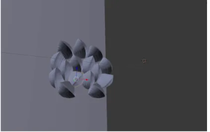
In this study, a Darrieus tidal turbine is considered according to the geometry built during the HARVEST program [3]. Blades are straight and built from a 0.032 m chord NACA0018 foil. The rotor is 0.175 m height and its diameter is 0.175 m (Fig.1). Laboratory tests have been performed in the current flume of LEGI and a motor is used to force the turbine rotation.
Figure 1: 3D view of the clean turbine
Air and water are used. Indeed, air is not realistic to study tidal turbines but easier to compute. Air calculation results are carried out using OpenFoam 2.3.0. In this version, PimpleFoam is based on a weak coupling between the fluid and solid parts. This gener-ates some convergence difficulties when the computation is realized with water where initial efforts are very important, leading the solver to diverge. A Reynolds similarity has been chosen to switch the simulation from water to air. Thus for water simulations, the following parameters are chosen : Uinf = 2.3 m.s−1 , ρ = 1025 kg.m−3 , ν = 1.3e−6 m2.s−1 for
water, and Uinf = 27.8 m.s−1, ρ = 1 kg.m−3, ν = 1.57e−5 m2.s−1for air. The solid’s
density is calculated to reach a rotation speed similar to the one imposed by the motor in laboratory experiments. It reaches 1300 kg.m−3for air calculations and 32500 kg.m−3for water. Blades are considered as rigid bodies.
Two different blade geometries have been modelled. The first is the clean blade previously described. The second is the same blade with a small colonization of the lower surface (Fig. 2). In order to study the impact of the mussel mass, a colonized blades case has been run under two different states: with and without taking the mussel mass into account. This way, the fluid dynamic and the mechanic effects can be uncorrelated. The mussel mass is taken into account considering that the solid density is uniform. The supplementary mass is only calculated using the added volume due to mussels.
Figure 2: CAD view of the modelled mussel colonization
In order to evolve from a forced rotation calculation to a flow induced one, both cases are computed and compared.
Numerical tests cases are summarized in Table 1.
Table 1: List of test cases with some details (Type of fluid, type of rotation, rotor mass, type of biofouling and type of mesh)
Simulation Fluid Rotation Mass (kg) Fouling Mesh Reference Case
(#1) Air Induced 0.085 None Coarse Forced Case
(#2) Air Forced None None Coarse Reference Water
Case (#3) Water Induced 2.131 None Coarse Forced water w.
Case (#4) Water Induced None None Coarse Small mussels w/o
mass change (#5) Water Induced 2.131 Lower surface Finer Small mussels w.
mass change (#6) Water Induced 2.185 Lower surface Finer In order to avoid side effects and capture the turbulent wake, the simulation channel is made as being the 4.6 rotor’s diameter large and 11 diameters long (Fig. 3). In [5], an AMI (Arbitrary Mesh Interface) cylinder was used to control the rotor’s rotation to avoid mesh deformation and re-meshing around blades. In order to reduce the number of nodes and the computing time, the refinement in the rotating zone is replaced by one tube of refinement zone around each blade to compute the efforts properly. Two meshes are used. A coarse mesh is employed for simulation using clean mesh (450 000 nodes), but this is insufficient to avoid numerical divergences on cases with mussels. Therefore, a finer mesh should be applied for cases with biofouling (900 000 nodes).
Figure 3: z-normal section of the computational domain with boundary conditions (in green). D is the rotor’s diameter in m. U is the flow velocity in m.s−1, P is the pressure in Pa and Plocalis the pressure at the calculated point closest to the wall.
3
Results
3.1
Model validation
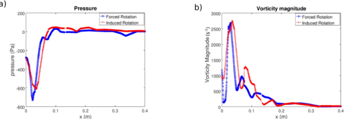
In order to validate the flow induced calculations, cases #1 and #2 are compared in two ways. First, pressure and vorticity are set side by side for the two cases in "Figure 4". Results are close. In this particular position (Fig. 5), a vortex is released by the blade, which implies high pressure and vorticity magnitude in this area. Vorticity is more representative of the fluid dynamic than the fluid pressure and allows to capture three different vertices in both cases. Pressure and vorticity values tend as expected towards zero in the far field.
Figure 4: Flow characteristics in the wake for forced (blue circles) and induced (red crosses) rotation: a) Pressure b) Vorticity magnitude
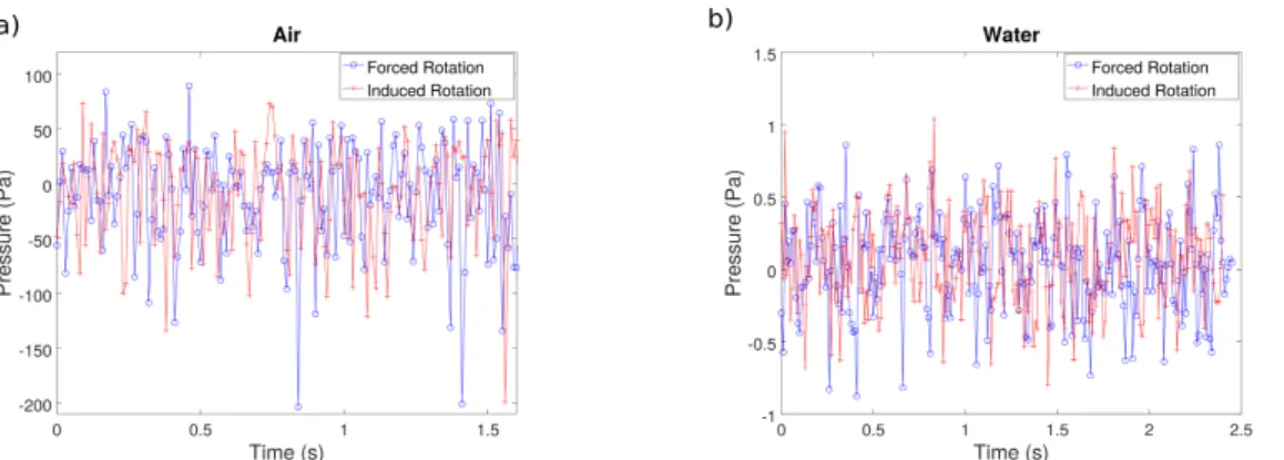
For cases #1, #2, #3 and #4, a probe is placed in the wake close to the rotor (represented as a white cross on "Figure 5"). Pressure and vorticity are plotted through the time on "Figure 6" and "Figure 7" . The signal is highly disturbed, especially in air cases. This can be explained by the high rotational velocity of the rotor around 44 rad.s−1. Results produced in case of a forced and induced rotation show high variability and comparable intensities. Once again, vorticity seems more efficient to represent flow behavior. Peaks are easier to recognise and
Figure 5: Hydrodynamic pressure over the computational domain (color scale). Blades are in white. The white transect represents the line where the results are plotted. Time series are extracted from the location represented by the white cross.
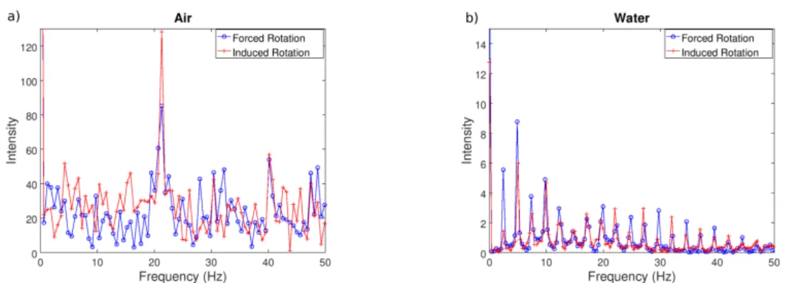
compare. This leads to calculate the vorticity variation in the Fourier space to confront their frequency spectra. The superposition of curves (Fig. 8) shows similarities. Frequencies of the main peaks are close in both cases. Some differences are mainly at low and high frequencies due to the small sampling (2 secs) and to the oscillating behavior of the rotor angular velocity for the induced case (Fig. 9). The results for #3 and #4 are even better where the FFT shows exactly the same peaks with some intensity variations. This can be explained by the lower rotation speed for water cases due to the coarse mesh.
Figure 6: Time series of the fluid vorticity at the probe location for forced and induced rotation for a) air b) water cases
On this basis, we conclude that the solid solver does not change fluid results. Because of the lack of experimental data, it is hard to validate the solid solver results. A mesh convergence trial is currently under way to define the best mesh. In parallel, laboratory tests are planned to have data with which to compare.
Figure 7: Same legend as "Figure 6" for the vorticity magnitude
Figure 8: Fluid vorticity spectra in case of forced (blue line with circles) and induced (red line with crosses) rotation for a) air b) water cases
Figure 9: Angular velocity for forced (blue line) and induced (red line) rotation for a) air and b) water cases
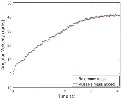
The rotor’s angular velocity is an ideal parameter to compare fouled cases. Its value takes mass variation and hydrodynamic into account. The rotor angular velocity of case #5 and #6 are plotted on "Figure 10". The mass effects are weak here because of the low variation of added volume (too small implantation). These test cases show mostly an increasing delay (from 0 to 0.01s) between the two rotors through the simulation. It can also be noticed that the general behavior of the rotor is slightly modified. This can be explain by the difference of impact of a blade on the others.
Figure 10: Rotor angular velocity according to time comparison between case #5 (unchanged mass) in blue and #6 (supplementary mussel mass) in red
The mass variation between #5 and #6 is only of 2.5% and delay can already be observed. Other variations are expected for more fouled blades such as the rotor angular velocity am-plitude or maximum. Other tests with big mussels (exaggerated scale) show an important difference between unchanged and modified masses. These results also show the limitations of a coarse mesh because the angular velocity changes drastically between the coarse case and the finer case.
3.2
Discussion
OpenFoam 2.3.0 seems to give correct results in the air for mechanic computation but the solver is unstable with water where the forces are more important than with air. OpenFoam 6.x is more suitable to compute mechanic calculations because of its strongly coupled solver. The different cases presented here will be migrated from the 2.3.0 version to the 6.x in order improve numerical convergence. Moreover during the tests a strong sensitivity to the mesh is observed: the calculation of forces requires a high resolution near the blades. Thus, a coarse mesh is not sufficient. A more accurate mesh should be adopted to compute forces with a better accuracy. This modification will strongly increase computation time. Conse-quently, a LES/Vortex Method coupling is being considered. The close field and mechanical computation will be solved in the same way as in this study, but far field will be computed using vortex particles.
As expected, biofouling seems to have a negative impact on the turbine’s performances through mechanical and fluid dynamical effects. In the case of a fully colonized rotor, fluid dynamical effects would be weak but mechanical effects should be high because of the supplementary mass. In order to validate results with a better accuracy, an experimental campaign with flow induced velocity is intended.
4
Conclusion
According to these article results, OpenFoam can be used as solver to compute fluid and solid motions. On the other hand, it is important to notice that the high mesh precision is fundamental for the FSI calculations. A finer mesh should be made for water cases. In order to compensate the increase of calculation nodes, a LES/Vortex particles is planned.
All current results suggest that biofouling has a negative impact on the performance of tidal turbines due to hydrodynamics and mechanics effects.
5
Acknowledgements
Authors are grateful to the "University de Caen Normandie (UNICAEN)" University for the financial support of these researches and to the CRIANN for the calculation facilities and technical support. I. Robin acknowledges the funding of his PhD on the impact of biofouling on tidal turbines by the "Région Normandie".
References
[1] Mohamed Titah-Benbouzid, Hosna Benbouzid. Marine Renewable Energy Converters and Biofouling: A Review on Impacts and Prevention. In EWTEC 2015, Proceedings of the 2015 EWTEC, pages Paper 09P1–4–2, Nantes, France, 2015.
[2] Aurélie Foveau and Jean-Claude Dauvin. Surprisingly diversified macrofauna in mo-bile gravels and pebbles from high-energy hydrodynamic environment of the ‘Raz Blan-chard’ (English Channel). Regional Studies in Marine Science, 16:188 – 197, 2017. [3] Ane Menchaca Roa. Numerical Analysis of Vertical Axis Water Current Turbines
[4] Shade Rahmawati. Study on Characteristics of Tidal Current Energy and Ocean
Envi-ronmental Pollution at Indonesia Archipelago. Theses, Hiroshima University, 2017. [5] Aurélie Rivier, Anne-Claire Bennis, Guillaume Jean, and Jean-Claude Dauvin.
Numer-ical simulations of biofouling effects on the tidal turbine hydrodynamic. International
Marine Energy Journal, 1(2):101–109, 2018.
[6] Yuanchuan Liu, Qing Xiao, Atilla Incecik, Christophe Peyrard, and Decheng Wan. Es-tablishing a fully coupled CFD analysis tool for floating offshore wind turbines.
Renew-able Energy, 112:280–301, 2017.
[7] J. Smagorinsky. General circulations experiments with the primitive equations. Monthly
Weather Review, 91(3):99–164, 1963.
[8] Christopher J. Greenshields. OpenFoam User Guide version 6, 2018.
[9] Erik Krane. A tutorial on modification of the turbofvmesh class for flow-driven rotation. 2015.
List of Figures
1 3D view of the clean turbine . . . 5 2 CAD view of the modelled mussel colonization . . . 6 3 z-normal section of the computational domain with boundary conditions (in
green). D is the rotor’s diameter in m. U is the flow velocity in m.s−1, P is the pressure in Pa and Plocal is the pressure at the calculated point closest
to the wall. . . 7 4 Flow characteristics in the wake for forced (blue circles) and induced (red
crosses) rotation: a) Pressure b) Vorticity magnitude . . . 7 5 Hydrodynamic pressure over the computational domain (color scale). Blades
are in white. The white transect represents the line where the results are plot-ted. Time series are extracted from the location represented by the white cross. 8 6 Time series of the fluid vorticity at the probe location for forced and induced
rotation for a) air b) water cases . . . 8 7 Same legend as "Figure 6" for the vorticity magnitude . . . 9 8 Fluid vorticity spectra in case of forced (blue line with circles) and induced
(red line with crosses) rotation for a) air b) water cases . . . 9 9 Angular velocity for forced (blue line) and induced (red line) rotation for a)
air and b) water cases . . . 9 10 Rotor angular velocity according to time comparison between case #5
(un-changed mass) in blue and #6 (supplementary mussel mass) in red . . . 10
List of Tables
1 List of test cases with some details (Type of fluid, type of rotation, rotor mass, type of biofouling and type of mesh) . . . 6