An Automated Confocal Micro-Extensometer Enables in Vivo
Quanti
fication of Mechanical Properties with Cellular
Resolution
OPENSarah Robinson,
aMichal Hu
flejt,
aPierre Barbier de Reuille,
aSiobhan A. Braybrook,
b,cMartine Schorderet,
dDidier Reinhardt,
dand Cris Kuhlemeier
a,1aInstitute of Plant Sciences, University of Bern, Bern 3005, Switzerland
bSainsbury Laboratory, University of Cambridge, Cambridge CB2 1LR, United Kingdom
cDepartment of Molecular, Cell, and Developmental Biology, UCLA, Los Angeles, California 90095 dDepartment of Biology, University of Fribourg, 1700 Fribourg, Switzerland
ORCID IDs: 0000-0001-7643-1059 (S.R.); 0000-0002-4308-5580 (S.A.B.); 0000-0002-6323-1979 (M.S.); 0000-0003-2440-5937 (C.K.) How complex developmental-genetic networks are translated into organs with specific 3D shapes remains an open question. This question is particularly challenging because the elaboration of specific shapes is in essence a question of mechanics. In plants, this means how the genetic circuitry affects the cell wall. The mechanical properties of the wall and their spatial variation are the key factors controlling morphogenesis in plants. However, these properties are difficult to measure and investigating their relation to genetic regulation is particularly challenging. To measure spatial variation of mechanical properties, one must determine the deformation of a tissue in response to a known force with cellular resolution. Here, we present an automated confocal micro-extensometer (ACME), which greatly expands the scope of existing methods for measuring mechanical properties. Unlike classical extensometers, ACME is mounted on a confocal microscope and uses confocal images to compute the deformation of the tissue directly from biological markers, thus providing 3D cellular scale information and improved accuracy. Additionally, ACME is suitable for measuring the mechanical responses in live tissue. As a proof of concept, we demonstrate that the plant hormone gibberellic acid induces a spatial gradient in mechanical properties along the length of the Arabidopsis thaliana hypocotyl.
INTRODUCTION
Understanding how gene activities are translated into shapes is still a major challenge. The key to deciphering this process is to have better insight into the role of mechanics (Moulia et al., 2011). Plant growth occurs by the yielding of the cell wall to stress (see Table 1 for definition of terms used) (Lockhart, 1965) and the direction of expansion is controlled by the relative properties of the tissue in the different directions. Altering these properties will lead to the formation of different shapes (Coen et al., 2004; Green et al., 2010; Kuchen et al., 2012). At the cell wall scale, these properties are primarily determined by the orientation of cellulose fibers (Probine and Preston, 1961; Green, 1962), which are deposited by cellulose synthase complexes that track along the microtubules (Paredez et al., 2006). Localized changes in the expression or activity of cell wall modifying proteins will alter the wall’s ability to expand and result in differential tissue deformation and, therefore, control morphogenesis (Fleming, 1997; Pien et al., 2001; Peaucelle et al., 2008).
Morphogenesis is also influenced by mechanical feedback. Plants are known to sense mechanical stress such as wind, gravity, bending, and even touch, and alter their growth ac-cordingly (Braam, 2005; Ditengou et al., 2008; Chehab et al., 2009; Richter et al., 2009; Band et al., 2012; Bastien et al., 2013). There is mounting evidence that plants can also sense internal mechanical stress, with microtubule orientation being reported to correlate with stress patterns (Hamant et al., 2008; Sampathkumar et al., 2014). Such internal tissue stresses typically arise due to the geometry of the tissue (Dumais and Steele, 2000; Hamant et al., 2008), different properties of cell layers (Hejnowicz and Sievers, 1995; Peters and Tomos, 1996; Kutschera and Niklas, 2007), or differential growth across a tissue (Coen and Rebocho, 2016); all of which are in turn controlled by mechanical properties (i.e., the stress-strain relationship for a material; Table 1). These internal stresses have also been proposed to influence morphology di-rectly by causing the tissue to buckle (Green, 1999; Green et al., 2010; Eldridge et al., 2016).
To fully explore how local wall properties translate into specific shapes and how they interact with gene regulatory networks, there is a need for techniques that enable mechanical properties to be quantified in developing tissues and responses to mechanical stress to be observed with high spatial resolution. Mechanical properties are intrinsically difficult to measure as force can only be measured by its impact on an object. The mechanical properties of a material describe how it deforms when a force is applied;
1Address correspondence to [email protected].
The author responsible for distribution of materials integral to the findings presented in this article in accordance with the policy described in the Instructions for Authors (www.plantcell.org) is: Cris Kuhlemeier (cris. [email protected]).
http://doc.rero.ch
Published in "The Plant Cell 29 (12): 2959–2973, 2017"
which should be cited to refer to this work.
formally, they describe the relationship between stress (force/ cross sectional area) and strain (relative change in length). Therefore, mechanical tests rely on precisely applying either a force or a deformation to a tissue and measuring the other property.
Many methods are available for measuring tissue level me-chanics in large samples, including extensometers. The classical extensometer setup involves clamping the sample, then applying a calibrated weight and measuring the deformation. The samples are typically millimeters to centimeters in length, and deformations are measured in the order of millimeters per hour. Extensometers were used extensively and most notably in the discovery of the cell wall modifying protein expansin (McQueen-Mason et al., 1992). Expansins were found to increase cell wall creep (i.e., the time-dependent irreversible strain that occurs when a constant force is applied). The irreversible component is calculated by removing the force and measuring the deformation that remains. This type of test is thought to best reflect the action of turgor on the cell wall. Extensometers have also been used to study elasticity (i.e., the ability to deform instantly and reversibly) and creep in etiolated Arabidopsis thaliana hypocotyl samples (Park and Cosgrove, 2012; Miedes et al., 2013). These experiments were conducted on dead tissue so that water movement and turgor would not be an issue and were boiled to inactivate endogenous enzymes and proteins. Extensometers typically provide organ level information.
Driven by the need to study mechanical properties with cellular resolution and in the smaller developing tissues of Arabidopsis, nano- and micro-indentation techniques have been adapted for this purpose. All of these methods involve indenting the tissue and measuring the force required to do so. Atomic force microscopy (AFM) is such a technique and was used to identify spatial differences in cell wall properties in the shoot apical meristem (Milani et al., 2011). These experiments were per-formed on plasmolysed tissue and involved very rapid in-dentations (30–80 mm s21) of 40 to 100 nm in depth using a tip with a radius of 10 to 40 nm. They provided very high spatial resolution, at the subcellular and cellular level. They were also able to relate cell wall stiffness directly with gene expression by aligning sequentially acquired AFM and confocal images with the aid of a fluorescence stereoscope (Milani et al., 2014). Similar experiments were conducted using 1-mm probes (Peaucelle et al., 2011) and further utilized to examine the effect of auxin on meristem cell mechanics (Braybrook and Peaucelle, 2013). Indenting with larger probes (5mm) has been proposed to provide information on inner layers (Peaucelle et al., 2011) or about the turgor pressure of the cells (Routier-Kierzkowska et al., 2012; Weber et al., 2015). Extracting cell wall or turgor pressure measurements from indentations requires sophisticated models that take into account parameters such as the relative contribution of the geometry and cell wall thickness (Weber et al., 2015; Malgat et al., 2016). Indentation measurements are also made perpen-dicular to the main direction of growth. This is appropriate for the study of the pectin matrix or turgor as they are isotropic; however, the other structural cell wall components such as cellulosefibers are highly anisotropic and it is less clear how this information should be interpreted (Cosgrove, 2016).
Indentation-based methods and extensometers provide very different information and operate at vastly different scales. Here, we propose a new technology; the automated confocal micro-extensometer (ACME). ACME can be used to measure mechanical properties and to apply mechanical stress. Designed to bridge the gap between conventional extensometers and indentation-based methods, ACME provides tissue and cellular resolution in-formation on the mechanical properties of small growing tissues such as in Arabidopsis. By facilitating mechanical measurements on developing Arabidopsis tissues, we expand the possibility of utilizing the vast array of knowledge and genetic tools that have been developed by the community.
Conceptually, ACME operates like a classical extensometer, but is much smaller, fully automated, and, crucially, relies on confocal images for strain computations. Therefore, strain is computed from features on the tissue itself. This improves the resolution, accuracy, and scalability of the measurement. The images enable cellular strain to be computed in 3D. The simul-taneous acquisition of images also enables responses to me-chanical stress and tissue health to be assessed continuously and in real time. Extensometers are naturally easier to couple to a confocal microscope compared with indentation devices, as they measure perpendicular to the imaging axis. Indentation methods by contrast obscure the image and must be used se-quentially (Milani et al., 2014; Louveaux et al., 2016).
We demonstrate the usefulness of ACME by investigating the response of light-grown Arabidopsis seedlings to the growth hormone gibberellic acid (GA). GA is known to promote a burst of growth in light-grown Arabidopsis hypocotyls (Sauret-Güeto et al., 2012). Studies in other species have demonstrated that GA acts to regulate growth via changes in the cell wall (Adams et al., 1975; Stuart and Jones, 1977; Cosgrove and Sovonick-Dunford, 1989; Taylor and Cosgrove 1989). Here, we study the mechanical changes that occur during the response to GA in the light-grown hypocotyl of Arabidopsis with cellular resolution.
RESULTS
Introduction to ACME
To measure a range of material properties, at different time scales, and with cellular resolution, we developed a miniature exten-someter which is mounted on a confocal microscope (Figures 1A to 1B). It is tailored for use on small samples (<2 mm), such as Arabidopsis seedlings, but could be adapted for larger samples and used in combination with other imaging systems. ACME is easily assembled from a combination of commercially available parts and custom parts (Supplemental Figure 1) which can be 3D printed (designs included; Supplemental File 1, 3D_printer_parts. zip) or as in Figure 1B cut from sheet aluminum (see Methods; Supplemental File 1, ACME_AssemblyGuide.pdf).
Like a classical extensometer, ACME enables measurements to be made parallel to the direction of growth. The sample is ma-nipulated using a robotic nanopositioner (Figures 1A to 1C, labels 4 and 5), which enables very small movements to be made with high accuracy (better than 50 nm). ACME measures forces using a load cell (a senor that transforms force into an electronic signal),
so that the force can be measured instantly and directly, rather than having to be computed. For this study, we used a 10 g load cell to enable forces to be measured within the physiological range for an Arabidopsis hypocotyl as determined by Miedes et al. (2013) (Figures 1A to 1C, label 3) and with low drift (<100mN per hour; Supplemental Figure 2). We typically measured and applied tensile forces between 1 and 10 mN (0.1–1 g). Custom software connects the positioner and the force measurement in a feedback loop (Figure 1C, label 14) so that a stable force can be maintained. To provide a positive user experience, fullflexibility in the type of experiment and to ensure reproducibility, the user can control ACME via small protocols that are defined in the parameterfile (see Methods; an example parameter file is in-cluded with the software https://github.com/ACME-Robinson/ InstallPackage). The user can specify a force or a deformation that should be applied, and the duration for which it should be maintained. Any number or combination of forces or deforma-tions can be specified. ACME will then perform these steps and record the force and position continuously (Figures 2A to 2F), allowing instant and direct measurements of force, rather than relying on post experiment computations. The user can specify the tolerance around the target force to prevent the sample being adjusted continuously. The user can also specify the maximum amount the robot can move at once to determine how quickly stress or strain is applied. The ability to perform a wide range of experiment types is important as biological materials are heterogeneous and their properties cannot be defined by a single experiment type.
ACME is sufficiently small and light to enable mounting onto a confocal microscope stage without obscuring the image or impacting the microscope function (Figure 1B, label 9). A custom base plate (Figures 1A to 1C, label 8) for secure attachment to the z-stage enables simultaneous image ac-quisition and mechanical measurements to be made. The images are used to compute strain/deformation more accu-rately compared with using the robot position, which is sen-sitive to any sample movement (Figure 2A). The images also enable responses to stress or strain to be observed at a cellular scale and in 3D.
Measuring Cellular Growth in Light-Grown Hypocotyls To demonstrate the usefulness of ACME for measuring me-chanical changes during early growth in light-grown hypocotyls, wefirst characterized their growth in the presence of either GA or the GA biosynthesis inhibitor uniconazole compared with control conditions. Confocal image stacks were collected for hypocotyls at different ages and treatments (see Methods). As hypocotyls are not always perfectly straight, a Bézier curve wasfitted to each hypocotyl image stack (Figure 3A). The curves were used to determine the length of the hypocotyls (Figure 3B), as well as to provide a positional reference system for each hypocotyl. GA-treated hypocotyls were much longer (2.33 mm6 0.18SE, n = 5) 5 d after stratification (DAS) compared with the control (1.23 mm6 0.05SE, n = 5) or uniconazole-treated hypocotyls
(1.05 mm6 0.05SE, n = 4) (Figure 3B). The majority of this growth
occurred between 2 and 3 DAS in GA-treated (2 DAS: 0.85 mm6 0.042SE, n = 12; 3 DAS: 1.8 mm6 0.08SE, n = 10; P = 2.85e-8) and
control seedlings (2 DAS: 0.79 mm6 0.03SE, n = 8; 3 DAS:
1.2 mm6 0.05SE, n = 6; P = 0.0001). Unless stated, all com-parisons were made using a Welch two sample t test. Uniconazole prevents germination, so seedlings were transferred to the uni-conazole at 2 DAS, which suppressed subsequent elongation (3 DAS: 0.97 mm6 0.04SE; 5 DAS: 1.05 mm6 0.05SE, n = 4; P =
0.26). The difference in hypocotyl length was significant between the GA and control treatments at 3 to 5 DAS (P < 0.001) but not at 2 DAS (P > 0.1). The uniconazole-treated hypocotyls were sig-nificantly shorter at 3 and 5 DAS compared with the control hy-pocotyls (P < 0.05).
To look at cellular growth, epidermal cell size was measured in 3D using the image analysis software MorphoGraphX (Barbier de Reuille et al., 2015). The volume of epidermal cells was extracted from the segmented images (Figure 3C) and displayed against relative position along the hypocotyl (Supplemental Figure 3A). A principal component analysis (PCA) was performed in MorphoGraphX on cell volumes to extract measures of cell length and diameter as follows: PCA enabled an approximation of each cell as a cylinder (Figure 3D) with PC1 corresponding to the length of the cell, and the average of PC2 and PC3 was used to ap-proximate the cell diameter (Figure 3E; Supplemental Figure 3B) (see Methods). We compared the length of cells from the above hypocotyls at different relative distances along the hypocotyl using the reference system from the Bézier curve (Figure 3F). At 2 DAS, when hypocotyl height was comparable (see above), mean cell length was not significantly different (P = 0.76) between control (25.5mm 6 0.41SE, n = 1115) and GA-treated hypocotyls (25.7
mm 6 0.46SE, n = 1887); by 4 DAS, the average length of cells was significantly larger (P < 2.2e-16) in the GA-treated hypocotyls (47.7 mm 6 0.49SE, n = 3226) compared with the control (32.5mm 6 0.45
SE, n = 1157). We extracted the change in average cell length along
the hypocotyl from 2 to 4 DAS by performing local polynomial regressionfitting on the data in Figure 3F. The GA-treated and control seedlings do not expand uniformly along their length (Figure 3G). In the GA-treated plants (blue line) the increase in cell length between 2 and 4 DAS was larger in the middle and upper parts of the hypocotyl, likely due to the cells in the lower part of the hypocotyl having already expanded more by two DAS. In control seedlings (red line) cell elongation was greatest in the middle of the
Table 1. Definitions of Terms Used
Term Definition
Stress The force acting on the material per unit area Strain The relative increase in length of the material;
can also be expressed as a percentage change in length
Mechanical properties
The stress-strain relationship for a material; if the same force is applied to a material that is twice as thick or twice as stiff, it will deform half as much, if the material is otherwise the same Elastic Elastic materials deform instantly and reversibly Creep Time-dependent irreversible strain that occurs
when a constant force is applied and maintained. Creep is measured using creep tests. A force is applied and maintained for a period of time. The force is removed to reveal the reversible and irreversible deformation.
hypocotyl. These data provide a framework in which to address how spatially variable growth depends on the local mechanical properties of the tissue.
Altering GA Increases Cell Wall Elasticity
We used ACME to determine if GA treatment altered the elastic properties of the cell wall. Elastic materials deform instantly when loaded, and upon unloading instantly return to their original size. By measuring the instantaneous deformation when a force is applied, we can compare the elastic properties of tissues. For this type of test, the samples were flash-frozen and thawed as by
Durachko and Cosgrove (2009) to diminish the impact of turgor and water movement. The samples were then rapidly loaded and unloaded multiple times. Interpreting such measurements re-quires accurate strain information. The position information from the positioner includes sample slippage, which would lead to an overestimation of the strain (Figure 2A). Instead, we computed strain from the confocal images using landmarks that we identified on the hypocotyl. As images were acquired continuously, gen-erating thousands of images for a single experiment, we de-veloped software (ACMEtracker) to compute the strain from those images. Two regions of interest are selected in thefirst image, usually cell junctions at either end of the sample. The software then
Figure 1. ACME Setup. (A) A diagram of ACME.
(B) Photograph of ACME mounted on a Leica SP5.
(C) Diagram of the control of ACME. The panels show the following: (1) the moving arm; (2) the measuring arm; (3) the force sensor (Futek LSB200 10 g load cell); (4 and 5) the nanopositioners (SLC1720s; SmarAct); (6) the dish for solution; (7) the sample mounting position; (8) the confocal mount; (9) a 203 confocal dipping objective (Leica); (10) load cell holder; (11) amplifier (Futek CSG110); (12) signal acquisition box (SCB68); (13) computer-based signal acquisition system (NI6221PCI); (14) custom-made software and SmarAct controller software library; (15) SmarAct MCS3D controller; (16) microscope (Leica SP5); and (17) confocal stage. ACME is a combination of custom and purchased components shown in dark and light gray, respectively. (1, 2, 8, and 10) Custom-made aluminum parts; (9, 16, and 17) microscope.
locates the regions of interest in subsequent images and extracts their coordinates (see Methods). From these coordinates, the oscillations were identified and the strain was computed using R scripts (Supplemental File 1, ExtractingOsc.R and oscillations.R). We compared the strain measured at 5 mN of force in samples of different ages and treatments. We found that strain (Figure 4A) was significantly higher (P = 0.04) in the GA-treated hypocotyls (14.3%6 1.7SE, n = 6) compared with control hypocotyls (9.6%6 0.80SE, n = 8) at 2 DAS. At 3 DAS, the difference between control
(9.7%6 2.7SE, n = 4) and GA-treated hypocotyls (11.6%6 1.21SE,
n = 6) was not significantly different (P = 0.47). Uniconazole-treated samples showed significantly less strain (7.9% 6 0.47SE
n = 6) compared with 3 DAS GA-treated hypocotyls (P = 0.026). We confirmed that GA increased tissue elasticity by performing AFM experiments; the apparent stiffness of 2 DAS (1.6 N/m6 0.04SE) and 3 DAS (0.52 N/m6 0.01SE) hypocotyls grown on GA (Figure
4B) was significantly lower (P < 2e-16, n > 300) than for the control hypocotyls (3.3 N/m6 0.04SEand 3.0 N/m6 0.03SE), consistent
with the higher strain measured with ACME at 2 DAS, but different than the 3 DAS ACME data. The elasticity data from ACME show a good agreement with the growth data (Figure 3B) as most growth occurs between 2 and 3 DAS. These data led us to conclude that GA increased cell wall elasticity coincident with increased growth in light-grown hypocotyls.
Measuring Strain Stiffening
Materials are usually not linearly elastic (Fung, 1993), meaning that the strain does not correlate in a linear manner with the amount of
force applied. The strain may increase more (strain softening) or less (strain stiffening) with increased force. Strain stiffening in the shoot apical meristem of Arabidopsis has been observed using osmotic treatments to induce elastic strain (Kierzkowski et al., 2012). A similar nonlinear elastic behavior has been reported in epidermal peels of maize (Zea mays) coleoptiles using an ex-tensometer (Lipchinsky et al., 2013). We tested if light-grown Arabidopsis hypocotyls show strain stiffening behavior by di-rectly applying a range of known forces to them and measuring the strain. We used frozen-thawed seedlings to avoid artifacts from turgor pressure, water movement, or feedback from me-chanical sensing. The average strain of 5 to 10 cycles of applying and removing force was plotted against the force applied (Figure 4C). The relationship between the force and strain was quantified byfitting linear and Hill-type models to the data and evaluating thefit (Table 2). The linear model had the form S5b$F 1 c, and the Hill function had the formS5a$ F
l 1 F, whereS is strain and F is
force. As both models have two parametersðb; c and a; lÞ, they can be compared by comparing the residual sum of squares (RSS). Although the amount of strain shown by the sample was variable, the behavior of strain against force was more consistent between samples of the same treatment. The stress-strain re-lationship of 3 DAS hypocotyls (Figure 4C) under all treatments was best described by a Hill function, which is indicative of a strain stiffening behavior. Taken with the existing literature, these results suggest that strain stiffening is a common property of plant tissues (Kierzkowski et al., 2012; Lipchinsky et al., 2013).
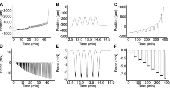
Figure 2. Examples of ACME Experiments.
(A) to (F) Robot axis position against time ([A] to [C]) and force against time ([D] to [F]).
(A) and (D) Oscillation experiments on 3 DAS GA-treated hypocotyls that were previously frozen then thawed. Initially (time = 0 min), there was a calibration step where the zero force was set and the plates moved to the user defined distance apart. The sample was then mounted and the experiment began. The force was applied in groups offive oscillations with a 30-s pause at zero force in between. At the end, the sample detached and the experiment stopped. Some slippage was apparent (t = 20 min), which is why material coordinates are used for the analysis of strain.
(B) and (E) A subset of the experiment shown in (A) and (D), displaying a single oscillation group.
(C) to (F) A representative multi-creep curve showing a thawed-frozen sample being repeatedly loaded and held at increasing forces before being returned to zero force.
Mechanical Measurements on Live Tissue
To be able to use the manyfluorescent markers available for vi-sualizing expression patterns or tracking subcellular structures and assess material properties of living cell walls, the sample must be kept alive. Therefore, we developed a method of attaching the samples to ACME so that they remain healthy and do not undergo strain prior to the experiment (see Methods; Supplemental File 1, Movie 1). Using this method, we were able to maintain healthy hypocotyl samples attached to ACME for at least 3 h. Sample health was evaluated in two ways. A healthy turgid sample at-tached to ACME took up water and generated a pushing force if constrained. When the sample was maintained at zero force, the positioner moved to maintain the force. For healthy samples, the positioner kept moving to allow the sample to expand (Figure 5A) and return the force to within the specified tolerance around zero
force (Figure 5B). Two GA-treated hypocotyls three DAS both exhibited 1% strain per hour in the 3-h period they were held at zero force. This is in comparison to the average 3% strain per hour that GA-treated seedlings showed between two DAS and four DAS (Figure 3B). The slightly lower value likely reflects the slowing of growth that seedlings show around 3 DAS. Strain was calcu-lated from the confocal images as the robot positioner results in this value being overestimated (4–5% per hour in this case). Sample health was also evaluated directly using the confocal coupling to observe the cells expressing a plasma membrane-localized GFP protein (Pro35S:PIN1-GFP). Counterstaining with propidium iodide (PI) was used to reveal dead cells (Figure 5C, arrow) and to stain the cell wall (Figure 5C). A healthy cell is visibly turgid; the membrane pushes against the cell wall leaving no visible gaps between the membranes of neighboring cells. When
Figure 3. The Growth Response to GA Is under Tight Spatial Control.
(A) A Bézier curve (red) wasfit to each hypocotyl image stack to allow accurate computation of hypocotyl length and to enable distances to be displayed in terms of distance along the hypocotyl.
(B) Lengths of hypocotyls in DAS grown in control conditions (Con) in the presence of GA or after being moved to uniconazole (Uni) (dashed line indicates seedlings approximate length before being moved). Bars indicate mean6SD(n$ 4).
(C) Cells were segmented in 3D from confocal image stacks and assigned a color and label for identification. Cells that were not segmented well were deleted or manually corrected. The volumes of the cells were extracted directly from the segmented image stacks. In order to extract the cell lengths and mean radii, the PCs of the cell volumes were extracted.
(D) Shows the same cells as in (C) but showing them approximated as cylinders so the PCs can be visualized.
(E) A diagram illustrating the principal components PC1 is the length of the cylinder and PC2 and PC3 are the diameters of the top of the cylinder. The cell length is taken to be the PC1, and the average of PC2 and PC3 is taken for the width. The high similarity between (C) and (D) shows that the approximation is good.
(F) Cell length, by position along hypocotyl, for control, GA, and uniconazole treatments at 2 and 4 DAS. The base of the hypocotyl just above the root is 0% and the top of the hypocotyl just below the cotyledons is 100%. The 99% confidence interval of the mean is shown for each curve (n $ 600 cells, from at least 4 hypocotyls).
(G) The relative change in cell length that occurs between 2 and 4 DAS for control and GA-treated seedlings is extracted from the data in (F). Bars = 100mm.
treated with hypo-osmotic mannitol concentrations, the cells can be seen to be visibly plasmolysed (Figure 5D) and some cells are damaged (arrow). In these cells, the plasma membrane is no longer visibly pushed against the cell wall and PI enters the nucleus. Based on these results, we concluded that healthy samples can be maintained in ACME and that samples damaged during mounting can be identified and removed prior to the experiment, thus en-abling mechanical measurements to be performed on live tissues. Creep Tests on Live versus Dead Tissues
To assess possible differences in mechanical properties between living and dead samples, we performed short creep tests on turgid, plasmolysed, or frozen-thawed hypocotyls from 3 DAS non-treated seedlings (Figure 5E). Creep tests look at the irreversible deformation of a material when held at a constant force. Creep is time dependent and can be observed over long time periods, enabling higher resolution images to be obtained. The strain was measured directly from 2D projections using ImageJ or point tracking software (Kuchen et al., 2012). The tissue layers of the hypocotyl are connected so the strain measured on the epidermis is equal to the strain across all of the layers. The strain observed reflects the properties of the whole tissue and will be most influenced by the load bearing layer of the tissue. The strain measured in the epidermis therefore provides a means of mea-suring the properties of the load-bearing layer, even without knowing the identity of that layer.
Creep tests were performed by applying 1 mN of force to the samples for 30 min then returning them to zero force again. Strain was computed relative to the sample length just before the force was applied. The samples did not show a significantly different amount of strain (turgid, 5.3%6 0.65SE; frozen, 4.6%6 0.22SE;
and plasmolysed, 4.3%6 0.28SE) after 30 min (P > 0.2, n$ 3);
however, in the turgid hypocotyls, the strain was more gradual, while in the other samples, the deformation was instantaneous (Figure 5E). Upon removal of the force, the turgid samples re-mained in the deformed configuration, indicating permanent deformation, and continued to elongate (5.9%6 1.04SE). In both
the plasmolysed and frozen-thawed samples, some of the de-formation was recovered, i.e., was reversible. Thefinal strain after 46.5 min was not significantly different between the plasmolysed and frozen-thawed samples (frozen, 2.2%6 0.19SE; plasmolysed,
1.2%6 0.52SE) (P > 0.1, n$ 3) but differed compared with the turgid samples (plasmolysed, P = 0.028; frozen, P = 0.067, n$ 3). This shows that water movement and/or metabolic processes likely played a role in the nonreversible extension we observed in the live turgid creep tests. Taken together, these data indicate that creep tests on turgid samples will yield mechanical data, which is different from that obtained from frozen-thawed or plasmolysed tissues, and data that are likely more relatable to the irreversible processes of growth.
GA Increases Creep in Live Tissues
To obtain physiologically relevant data of the growth response to GA, we performed creep tests on live two DAS light-grown seedlings. The samples were tested just before they would have undergone a burst of GA-induced growth if treated. The samples were maintained at zero force for 30 min to allow recovery from the sample preparation and to ensure they were healthy. Samples were then subjected to 1 mN of force for 2 h before being returned to zero force for 30 min (Figure 5F). Confocal images were acquired every 5 to 15 min and used to track the strain. The uniconazole-treated hypocotyls showed less total strain (during the 180-min observation period; 2.6%6 0.4SE, n = 4) compared with control
(7.3% 6 1.7 SE, n = 8; P = 0.077) and GA-treated samples
Figure 4. GA Increases the Elasticity of Hypocotyls.
(A) and (C) Hypocotyls were frozen and thawed then subjected to cycles of application and removal of force (Figures 2B and 2E).
(A) The average magnitude of strain incurred by 2 (2d) and 3 DAS (3d), control (Con), and GA-treated seedlings, and uniconazole (Uni)-treated seedlings at a force of 5 mN is shown. Bright-field images were collected every 645 ms, and strain was computed from regions that were tracked in the images using the ACMEtracker software (see Methods). Bars show means6SE(n$ 4, at least five oscillations were made). The strain for 2d GA differs significantly from the 2d Con (P = 0.041), and Uni differs from 3d GA (P = 0.025).
(B) AFM-based elastic stiffness obtained from living, plasmolysed, and 2 and 3 DAS seedlings, control, or treated with GA. Bars show means6SE. For each hypocotyl, three areas of 503 100 mm were indented from at least two independent samples. GA and Con differ significantly at 2 d (P < 2e-16, n > 400) and 3 d (P < 2e-16, n > 300). Different letters indicate means differ significantly (P < 0.05).
(C) Average strain was computed from rapid oscillation at a range of forces for 3 DAS seedlings. As above, batches of 5 to 10 oscillations were made with 30 s at zero force in between forces (as shown in Figures 2A and 2D). Strain was computed from images as described for (A). The force strain curves were compared with a linear and Hill-type model (Table 2).
(12.6%6 2.8SE, n = 8; P = 0.015) as evaluated using
repeated-measures linear mixed models (see Methods). The difference between control and GA-treated samples was not significant (P = 0.356, n = 8), perhaps due to the spatial restriction of the cells that elongate in response to GA (see next section). Upon removal of the force the samples remained strained, i.e., it was irreversible. These results confirm that inhibiting GA altered the mechanical properties of the cell wall at the organ scale in physiologically relevant conditions.
3D Cellular Resolution Strain Measurements
When force is applied to a sample, the force is equal at any point along its length (Landau and Lifshitz, 1986). Therefore, the dif-ference in strain of the cells in response to external force can be used to compute their material properties. If a cell strains more than another when experiencing the same stress, then it is more extensible. We performed additional creep tests using 10 mN of force on live hypocotyls, and high-resolution images were col-lected every 5 to 10 min. The images were segmented in 3D and cellular volume changes were computed (as for the growth analysis; Figure 3). All cells that could be segmented in the images were used. PCA was performed to approximate the length and diameter of cells (average of depth and width) (as in Figure 3E). The strain of the cells was computed at the end of the creep phase. Samples that detached, died, or underwent plasmolysis were excluded from the analysis. The strain in diameter was close to zero and often negative (Supplemental Figure 4A). The cells of the three DAS GA-treated samples showed a greater amount of strain in the middle and upper parts of the hypocotyl compared with the lower part (Figure 5G). The gradient in cell properties in the three DAS GA seedlings was seen in five out of six samples (Supplemental Figures 4B to 4E); one sample did not show the gradient as it was curved at the start of the experiment so the gradient in strain was greatest across the sample as the curved side straightened out (Supplemental Figure 4F). Control hypo-cotyls did not show such a gradient (Figure 5H) in thefive seedlings that were analyzed. The gradient in strain along the length of GA-treated hypocotyls showed good agreement with the ob-served growth pattern (Figure 3G). We confirmed that the ob-served gradient in strain was not a consequence of there being a difference in the cell wall thickness, by making sections at different positions along the hypocotyl (Supplemental Figures
5A to 5L) and analyzing them by transmission electron mi-croscopy (TEM). If the cell wall was thicker at the base of the hypocotyl, then the stress would be lower and this could explain the results without a change in cell wall properties. However, the cell wall was thinnest at the base of the hypocotyl (Supplemental Figure 5M) where there was the least amount of strain. These results show that there is a gradient in cell wall properties along the length of the GA-grown hypocotyls that correlates with the observed growth pattern.
Other Tissues
ACME can be applied to tissues other than hypocotyls. The mechanical properties of any tissue that is smaller in one di-mension compared with the other two, i.e., not spherical, can be measured using ACME. We demonstrated this using Arabidopsis cotyledons (Figure 6). Cotyledons are another system where mechanics has been of interest lately (Sampathkumar et al., 2014; Bringmann and Bergmann, 2017). When attaching to ACME, the entire seedlings remained intact and one of the cotyledons was placed between the plates. The samples were healthy before (Figures 6A and 6B) and after (Figures 6C and 6D) the application of stress, as demonstrated by the failure of PI to enter the cells and the plasma membrane being pushed tightly against the cell wall. The deformation of the epidermal cells that occurred during the experiment was visualized by overlaying the before and after images (Figures 6E and 6F). The pavement cells can be clearly seen to have strained in the y axis, computed as 5% strain using the point tracker. We conclude that ACME is suitable for in-vestigating mechanical properties and feedback regulation in live cotyledons.
DISCUSSION
ACME is a versatile tool for quantifying mechanical properties in small tissues. It can be easily modified for use with a range of microscopes, enabling information to be obtained at different resolutions. ACME’s reliance on confocal imaging and image analysis tools for computing mechanical properties make it more accessible to biologists who are often more familiar with imaging techniques than mechanics.
ACME allows for the measurement of both elastic strain and creep (time-dependent, irreversible deformation) at the organ and
Table 2. Evaluating the Strain Stiffening Behavior by Model Fitting
Linear Model Parameters Hill Model Parameters
Treatment Best Model b c RSS a l RSS
3 d Con Hill 6.32e-6 0.060 0.0502 0.133 1653 0.0478
3 d GA Hill 7.54e-6 0.067 0.0351 0.157 1856 0.0285
Uni Hill 6.81e-6 0.033 0.0057 0.124 3049 0.0041
Model comparisons of linear versus Hill-type equation were performed for the oscillation data on the 3 DAS samples for the different treatments. The linear model has the formS5b$F 1 c, and the Hill model has the form S5a$ F
l 1 F, whereS = strain and F = force. The model fitting is done using
the nonlinear least squares method in R. As both models have two free parameters, the model that bestfits the data is selected based on it having the smallest RSS (underlined).
individual cell levels. We demonstrated this by measuring the change in these mechanical properties in response to GA in light-grown hypocotyls. Notably, we were able to reveal cellular res-olution spatial gradients in the cellular mechanical properties that were similar to the pattern of GA-induced growth. Measurements
with ACME and AFM are different in the type of information they provide. However, we saw a similarity in their measurement of elasticity in GA-treated hypocotyls. An important advantage of ACME over indentation methods is that mechanical properties are measured in the plane of growth. As ACME can provide cellular
Figure 5. Utilizing Confocal Images to Compute Mechanical Properties.
(A) and (B) A healthy, turgid, 3 DAS, GA-treated sample was held at zero force for 3 h. The relative position of the plates (A) and the force (B) are both recorded. The sample continued to generate a pushing force (A), and the plates moved to extend the sample and return the force (B) to within the range of tolerated forces (60.1 mN).
(C) and (D) The attachment of ACME to the confocal enables cells to be manually inspected in order to assess their health.
(C) A turgid hypocotyl after a creep experiment in water (as in [E]). Staining with PI (red) reveals a single dead cell (arrow). PI is excluded from healthy cells and stains the wall. The cells are turgid as the plasma membrane localized Pro35S:PIN1-GFP (green) reveals that the plasma membrane is in contact with the cell wall (red).
(D) Cells plasmolysed in 0.5 M mannitol have visibly lost contact between the membrane (green) and wall (red), mimicking the expected result for non-turgid and unhealthy cells. Dead cells lost GFP expression and PI entered (arrow).
(E) Creep tests were performed to compare live seedlings, thawed seedlings that had previously been frozen, and seedlings plasmolysed with 0.5 M mannitol. The samples were loaded with 1 mN of force at time zero and unloaded after 30 min (dashed lines). The deformation of the live samples was irreversible, while in the other samples, it was partially reversible. Strain was computed from confocal images that were acquired every 1.5 min. Data points show mean6SE(n$ 3). After 30 min, the strain was not significantly different between the samples (P > 0.2); at the end of the experiment, the strain differed
between the turgid samples and the other samples (plasmolysed, P = 0.028; frozen, P = 0.067).
(F) Creep tests were performed on live turgid two DAS seedlings grown in the presence of GA or control conditions and plants grown on uniconazole. Dashed lines indicate addition (30 min) and removal (150 min) of 1 mN of force. Strain was computed from confocal images that were acquired at a minimum of every 15 min. Data points show mean6SE(GA and control, n = 8; uniconazole, n = 4).
(G) and (H) Creep tests were performed by applying 10 mN of force to 3 DAS live, turgid samples. Z-stacks were acquired and the images were segmented. Corresponding cells were colabeled before and after stress was applied. Using PC analysis, the length of the cells was computed (as in Figures 3C to 3E) and used to compute the strain in length (%) per cell, shown as a heat map.
(G) The GA-treated sample showed a spatial gradient in percentage strain along its length. (H) The control samples do not show such a gradient in longitudinal strain.
Bars = 50mm in (C) and (D) and 100 mm in (G) and (H).
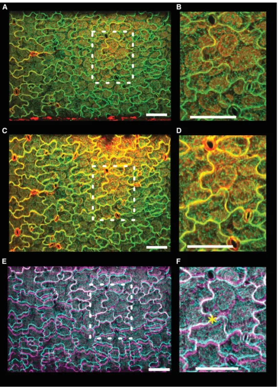
Figure 6. Using ACME to Apply Stress to Cotyledons.
A cotyledon was mounted onto ACME. The sample expresses the MBD-GFP marker (green) and was stained with PI (red) to demonstrate that the cells are healthy.
(A) and (B) Image of the cotyledon obtained with the 203 objective before application of 5 mN of stress in the y direction ([B]; enlargement of boxed region in [A]).
(C) and (D) After application of stress ([D]; enlargement of boxed region in [C]). The sample remains healthy, the cells are turgid, they continue to express GFP, and PI does not enter the cells.
(E) and (F) Before and after images appear very similar; however, by overlaying the GFP images (before, cyan; after, magenta), we can see the deformation ([F]; enlargement of boxed region in [E]). The images were aligned at an arbitrary point in the center of the image (asterisk) using MorphoGraphX. Opacity was adjusted to enable both images to be seen. Bars = 100mm.
scale information, it enables an easier comparison of the different methodologies that could yield great insight into how growth is regulated. Furthermore, exploring how each of these properties relates to growth in a living system is another advantage of the ACME system.
In addition to measuring mechanical properties, there is a great interest in the community to look at mechanical feedback. A range of methods have been used to demonstrate that plants respond to mechanical stress. These include making cuts or ablations (Hamant et al., 2008; Sampathkumar et al., 2014), os-motic stress (Nakayama et al., 2012), compressing the tissue (Nakayama et al., 2012; Sampathkumar et al., 2014; Louveaux et al., 2016), or large-scale deformations (Bringmann and Bergmann, 2017). These methods also induce other types of stress to the tissue, for example, wounding or drought. In many cases, the magnitude of the stress being applied is unknown or has to be deduced from models, and none of them allow for simultaneous imaging of the tissue. If the details and relevance of mechanical feedback are to be worked out, there is a need for methods that enable application of quantifiable stress within the physiological range. ACME provides the opportunity to do this.
METHODS
ACME Hardware
The extensometer is based on two SLC1720-S nanopositioners (Figures 1A to 1C, labels 4 and 5; SmarAct). The positioners are operated by custom-made software (Figure 1C, label 14) (available at https://github. com/ACME-Robinson/InstallPackage) via a SmarAct MCS-3D (SmarAct GmbH) controller (Figure 1C, label 15), which comes with its own software library. One of the positioners is driving the moving plate of the exten-someter responsible for exerting force on the sample (Figures 1A to 1C, label 5), while the other positioner (Figures 1A to 1C, label 4) is responsible for the vertical motion of the main extensometer body to allow re-placement of Petri dishes. The force measurement system consists of a force sensor (10 g load cell; Futek LSB200) (Figures 1A to 1C, label 3), its dedicated amplifier (Futek CSG110) (Figure 1C, label 11), and a com-puter-based signal acquisition system (NI6221PCI; Figure 1C, label 13 with SCB68 breakout box and label 12; National Instruments). The force sensor is attached to the sensing plate (Figures 1A and 1C, label 2) of the extensometer. In contrast to the moving plate (Figures 1A to 1C, label 1), the sensing plate is not actuated; instead, it is attached to a force sensor that measures force exerted on the plate by the sample. The load cell amplifier drives the load cell and picks up the force signal from the sensor. Amplified force signal from the amplifier’s output is delivered to the signal acquisition card for sampling. The load cell amplifier is wrapped in insulating foam to stabilize its temperature and therefore to minimize drift. The signal acquisition card mounted inside of a Linux PC is controlled by comedi library (http://www.comedi.org/) (linux control and measurement device interface). The comedi library provides soft-ware calibration solution using internal calibration reference of the NI6221PCI card. The force signal is sampled at 10 kHz frequency, software-calibrated, and then averaged in a 200-ms window (aver-age of 2000 volt(aver-age samples). Then, the aver(aver-aged volt(aver-age is offset-corrected (tare) with a value obtained during sensor tare at the beginning of the experiment. The offset-corrected voltage is converted into force by multiplying it by a gain factor (NV21) obtained during calibration of the force measurement system. The obtained force F (mN) is therefore F¼ gðV 2 V0Þ , where g is the gain (mNV21), V is the measured voltage (V), and V0is the offset voltage (V). The MCS Control Library,
which controls the SmarAct nanopositioners, is supplied by the manu-facturer. The extensometer plates (Figures 1A to 1C, labels 1 and 2) as well as all its other components (Figures 1A to 1C, label 8, and Figure 1C, label 10) are custom-made out of readily available aluminum profiles and assembled with standard screws and nuts. They can also be 3D printed (Supplemental File 1, 3D_printer_parts.zip). A detailed assembly plan for ACME is included (Supplemental File 1, ACME_AssemblyGuide.pdf).
ACME Control Software
The hardware is directly controlled by accompanying libraries, which we interface through the custom-made ACMErobotX software (Figure 1C, label 14). We also developed the ACME software to perform higher level functions (both software packages are available at https://github.com/ ACME-Robinson/InstallPackage). To aid the user, we have also included an example parameterfile in the repository, where the user can easily specify the key features of the experiment without any knowledge of coding. The parameterfile is where the user can specify other features, for example, the speed of movement of the robot, the initial gap size (i.e., how far apart the plates are at the start of the experiment), or the location to save the data. To further aid the user, the robot position and measured force are saved continuously as a csvfile and can be viewed in real time or analyzed later. The csv file includes the following headings: LoggerTime(ms), X_Position(mm), Y_Position(mm), IndentationForceSensor_Force(mN), and ProtocolFlag(flag). The first column records the time, the second and third record the position of the axis, and the fourth records the force. The protocolflag can be used to separate the different stages of the experiment, notably the initial step where the force is set to zero and the arms move apart prior to sample attachment.
ACME Calibration
The force sensor (load cell) is calibrated by detaching it from the exten-someter and vertically mounting it on a stand. Weights are placed on top of the load cell in a sequence and their corresponding digitized voltages are acquired, as seen by the software. Least squares linearfitting provides the slope of the voltage-to-force relationship, which we call sensor gain, expressed in NV2 1. The gain value is later used by the software to compute force inmN from the acquired voltage values (see Supplemental File 1, ACMECalibrationGuide.pdf and calibration_worksheet.odt). The aim of the calibration procedure is to determine the overall gain (scaling) of the force measurement system. The input is a series of weight readings of test weights measured with precise laboratory scales. This information is entered into the robot.inifile before the first use of the equipment. Drift was measured by holding the position of the plates and measuring the force. Fifty-one runs were performed sequentially. It was found that drift was highest in thefirst run but after this it dropped to below 100 mN per hour (Supplemental Figure 2). This is 10% of the smallest force typically applied. Dimensional changes to the sample result in varying force being exerted on the extensometer plates (;1.7 mm for 1000 mN).
ACME Protocols
ACME protocols are defined as sequences of steps, where each step defines a desired position or force and duration, as described by parameters. Parameters have the following form: force or position F/P instructs the system to move to achieve a target force or a target position. The position is relative to the previous position while the force is compared with the zero force set at the start of the experiment. The magnitude of force or the position is then given; position is inmm and force is in mN. The length of time to hold the new force or position is then given in seconds. At all times, the force and position are recorded. The plates continue to be adjusted to maintain the force if it goes outside the threshold specified.
Usually a threshold of 100mN is used as this is comparable to the drift that we observed. The step size is also specified and can be altered depending on the size of the deformation or the property of the material. Usually a step size of 2mm is used. The initial gap size is also specified. The plates move to this initial position before the experiment starts and the averaged voltage offset is obtained to tare the sensor. The sample is mounted and then the user defined protocol is implemented.
Example Creep Protocol
The following example is of a creep test as performed in Figure 5F. Steps are specified; F or P denotes force or position. The third parameter is the mag-nitude, with negative force values denoting tension and positive values de-noting compression. The fourth parameter is time in seconds. In this example, the plates move to achieve zero force, which is held for 1800 s (30 min), then the plant is stretched until a force of 1000mN is exerted on the load cell, and this is held for 7200 s (2 h). The force is then returned to 0 and then held for another 1200 s (20 min): Step, F, 0, 1800; Step, F,21000, 7200; Step, F, 0, 1200.
Oscillation Experiments
Samples were rapidly loaded and unloaded. Samples were held at the stated force for 1 s. Five to ten oscillations were made at each force and then the sample was held at 0 force for 30 s. Then, a new batch of oscillations was performed. Bright-field images were collected every 645 ms, and the images were opened in the ACMEtracker (software available at https://github.com/ACME-Robinson/InstallPackage) and two regions of interest were selected. These regions were tracked in sub-sequent images using a normalized cross correlation coefficient method. The coordinates were written to afile and used to compute strain per batch of oscillations using R scripts (Supplemental File 1, ExtractOsc.R and oscillations.R). For 2 DAS oscillation experiments, at least seven samples were tested per treatment, and for 3 DAS and the uniconazole treatment, at leastfive samples were tested. The data from the replicates were combined using the stat_smooth function of ggplot2 in R.
To test the competing hypothesis of a linear slope versus a Hill function for the strain force relationship in the oscillation experiments, wefitted both models using a least square estimate. As it was not possible to apply as high a force to the 2 DAS samples as it was to the 3 DAS samples, the model was alsofitted to a subset of the three DAS data to match the range for the 2 DAS samples. The force and strain data for the experiments were separated by treatment and age andfitted using the nonlinear least square method in R (nls). The linear models had the following formS5b$F 1 c, whereS is strain and F is force with starting parameters b = 0.1, c = 0. The Hill function has the form:S5a$ F
l 1 Fwith starting parametersa = 0.1 and l =
1000. Thefitted values and residual sum of squares can be found in Table 2. As both models have two free parameters, we can compare the RSS tofind the model that bestfits the data.
Live Creep Tests
Live samples were mounted without glue and held at zero force for 30 min then at 1 mN for 2 h and then returned to zero force for 30 min. Confocal z-stacks were collected regularly. A projection was made from the stack in MorphoGraphX and exported. Cells of interest were tracked using the Point tracker as by Kuchen et al. (2012). The strain was computed manually form these measurements. Cells were selected that were as far apart as possible and vertically aligned. For the comparison of live, plasmolysed, or frozen tissue, samples were kept alive in water, treated with 0.5 M mannitol, or flash-frozen in liquid nitrogen and stored at –80°C, then thawed prior to testing. For each treatment, three samples were tested, with images ac-quired every 1.5 min. Strain was compared after 30 min and at the end of the experiment, using the Welch two sample t test.
For the creep tests on live samples, eight seedlings were used for GA and control conditions and four seedlings for the uniconazole condition. The results were analyzed by constructing repeated measure models using the lmer function of the lme4 package in R with strain as the response variable and treatment as afixed factor. We allowed change in strain over time to differ across individuals. Strain and time were ln transformed to meet the assumptions of normality and linearity. Significance was de-termined with linear mixed modelfit by REML t tests, using Satterthwaite approximations of the degrees of freedom (lmerTest function). Two models were compared:
M1←lmerðStrain ; Time þ treatment þ Time : treatment þ ðTimejsampleÞ; data ¼ dataÞ
M2←lmerðStrain;Time þ treatment þ ðTimejsampleÞ; data ¼ dataÞ The models were compared using a log likelihood test and no significant difference was found (X2= 1.39, df = 2, P = 0.499), so the simpler model
(M2) was used. Compared with the control treatment, the GA-treated samples did not differ (df = 17, t = 0.948, P = 0.356), and the uniconazole-treated samples showed a significant difference when compared with the control samples (df = 17, t =21.880, P = 0.0774). When only GA- and uniconazole-treated samples were compared, the models were also equivalent (X2= 1.187, df = 1, P = 0.276). The GA and uniconazole
treatments differed significantly from one another (df = 10, t = 22.926, P = 0.0152).
Cellular Resolution Creep Tests
Samples were held at zero force for 15 min, 10 mN for 30 min, then returned to zero force for 20 min. Confocal z-stacks were collected and segmented as described for the growth measurements. Corresponding cells were then identified in subsequent images and given the same label. The change in cell size was computed to give cellular strain values. All cells that could be segmented in the images were used. Samples that detached, died, or underwent plasmolysis were excluded. The gradient in cell properties in the 3 DAS GA seedlings was seen infive out of six samples; one sample did not show the gradient because it was curved (Supplemental Figure 4).
Plant Material, Growth Conditions, and Imaging
Seeds were surface sterilized and sown on MS medium (4.4 gL21Murashige and Skoog salts [Sigma-Aldrich], 0.5 gL214-morpholineethanesulphonic acid [Sigma-Aldrich], and 0.8% agar, pH 5.7), with the possible addition of 10mM GA3(Sigma-Aldrich; 48880) or 2mM uniconazole (Sigma-Aldrich;
19701). Plants grown in the presence of uniconazole were germinated on control media and then transferred to the uniconazole after 2 d. Plants were imbibed in the dark at 4°C for 2 or 3 d and then grown in controlled environment chambers (100mE continuous light conditions using Philips TL-D super 80 58W/830 and 840 bulbs, at 22°C) as by Sauret-Güeto et al. (2012). The Pro35S:PIN1-GFP line from the Benkova lab and Pro35S: GFP-MBD line (Hamant et al., 2008) were used as membrane markers. Samples were stained with 0.1% PI to stain cell walls and highlight dead cells.
Images were acquired using a Leica SP5 with a HCX APO L 203/ 0.5-W objective and a Leica HyD hybrid detector. GFP was excited using a 488-nm laser and detected at 490 to 540 nm. The laser power was maintained as low as possible. For oscillation experiments, images were collected in a single z-plane using the bright-field de-tector for rapid imaging. For growth curves and creep tests, z-stacks were collected. To enable cell segmentation in MorphoGraphX a z-step of 0.4 to 0.5mm was used, with a scan speed of 400 Hz and no scan averaging.
Growth Analysis
Cell volume and length calculations were made using a version of MorphoGraphX (http://www.lithographx.org/), which contains the necessary processes. The image stacks were loaded into MorphoGraphX and segmented by the following procedure: a gaussian blur of size (1, 1, 1), autoscaling of the stack, and ITK autoseed segmentation with a threshold of between 1000 and 1500 depending on the sample. Any over-segmented cells were then merged. Under-segmented areas were deleted, as were cells from the internal layers, those that were not completely visible in the image, or those that were part of the stomata lineage as their size does not reflect that of the growth rate of the plant, but is under different regulation. Marching cubes of size 2 was performed without smoothing. A Bézier curve of order 5 was fitted to the sample (Figure 3A), arc-length parameterized, with the zero set to a defined pointalongthehypocotyl. Thehypocotyllength wasextracted from the Bézier curve. The position of a cell along the hypocotyl is then defined as the curve parameter of the projection of its center onto the Bézier curve. For each cell, we computed its volume, length, and mean radius. The volume could be estimated directly from the image. The length and mean radius were computed byfirst extracting the principal components (PCs) of the cell shape. The main one corresponds to the direction of the length and 2nd and 3rd to the width and height (Figure 3E). The distance along a PC was measured by projecting the voxels defining a cell onto the direction and taking the distance between the 0.5 and the 99.5 percentiles. The mean radius is then the average of the lengths along the 2nd and 3rd axes. Any cells not well represented were deleted. Graphs were produced using ggplot in R; the stat smooth function was used tofit a confidence interval with 99% level. Local polynomial regressionfitting was performed on the cell length data using the loess function in R. The output of thisfitting was used to compute the difference in length of cells at the different time points.
Sample Attachment
Entire seedlings were attached without crushing the tissue (Supplemental File 1, Movie 1). The experiments were conducted in distilled water to prevent sample drying. The attachment of the sample to the movement arm was made using tough tags (0.943 0.50 inches, white, catalog no. TTSW-1000; DiversifiedBiotech). They are waterproof and remain attached to the robot arm, even when immersed in solution. Samples remained healthy for many hours and can be tested with forces in the 1 to 2 mN range. For higher force measurements ($5 mN), a thin layer of cyanoacrylate glue was added to the tape (Supplemental File 1, Movie 2); under this condition, the sample remains healthy for shorter periods of time. Sample health was assessed visually; samples were regarded as healthy if plasmolysis did not occur. Sample health could also be measured by monitoring the force; a healthy sample will exert a force if held at afixed position and will expand if actively maintained at zero force. Cyanoacrylate glue is suitable for previously frozen tissue or for short experiments with high force.
AFM Sample Preparation and Analysis
Plants used for AFM experiments were grown as described above except in long-day conditions. Immediately preceding AFM analysis, each batch of seedlings was dissected, on moist paper towels, to remove the cotyledons. Dissected hypocotyls were then placed on etched glass slides and secured between glass bumpers with 0.8% low melting point agarose in 0.55 M mannitol. Once secured, the samples wereflooded with 0.55 M mannitol to suppress turgor pressure. Samples were left to plasmolyze for a minimum of 20 min. All solutions were prepared using ultrapure water at pH 7.1.
Dissected and plasmolyzed hypocotyls were indented using a Nano Wizard 3 AFM (JPK Instruments) mounted with a 0.8-mm diameter rounded indenter (Windsor Scientific) on a cantilever of 40 N/m stiffness. Cantilever stiffness was determined by thermal tuning prior to experiment initiation.
Tip sensitivity was calibrated byfirst performing indentations on a clean glass slide. For each hypocotyl, three areas of 503 100 mm were indented with 323 32 points: A top area near the cotyledons, a middle area, and an area just before the collet. Positions of each grid were recorded with a top-view camera. Indentations were performed with 1000 nN of force yielding an indentation depth range of 250 to 500 nm, and a total of 1024 in-dentations were performed per area per biological sample.
AFM Data Analysis
Force indentation curves were analyzed using JPK SPM Data Processing software (JPK Instruments; DE, v. spm 4.3.10) using the following steps: Voltage readings were converted to force using calibrated sensitivity and cantilever stiffness values, baseline subtraction and tilt correction were applied to curves, vertical displacement offset adjustment was used to center the non-contact force to zero, indentation was calculated by subtraction of cantilever bending from piezo position during indentation, and the elastic stiffness was calculated byfitting a tangent to the final 150 nm of the indentation. Extraction curves were not analyzed due to numerous adhesion difficulties during tip removal from the surface. Fitting the last 150 nm of the indentation ensured that stiffness values reflected a linear elastic constant and avoided possible contact area evolution during the beginning of the indentation. Elastic stiffness maps were then imported into MatLab, and values were selected from anticlinal cell walls only. Anticlinal walls were used for the following reasons: Often surface walls buckled or showed complex force-deformation curves due to geometrical instability without turgor support, anticlinal walls maintained relatively constant depth during cell elongation allowing for comparability across cell sizes, and anticlinal wall indentations were more normal to the indenter axis than curved surface walls. For each grid area, 30 to 50 points were chosen from anticlinal walls and used for subsequent analyses, representing data from 3 to 10 cells depending on cell length in the scan area.
Cell Wall Thickness Measurements
Seedlings werefixed in 50 mM Na-cacodylate buffer, pH 7.4, with 2% (v/v) glutaraldehyde (EMS) for 2 h at room temperature. After six washes with 50 mM Na-cacodylate, the samples were postfixed overnight with 1% (w/v) OsO4in Na-cacodylate buffer at 4°C. After six washes in cacodylate buffer and one wash with water, the samples were dehydrated through an ac-etone series (10%, 20%, 30%, 50%, 70%, 90%, and 100%, each 10 min) and seven subsequent changes of acetone. Embedding proceeded by soaking in increasing concentrations of Spurr’s resin (Plano) in acetone (25% 1.5 h, 50% 1.5 h, 75% overnight, and 100% 6 h) and polymerization at 70°C for 18 h under dry atmosphere (silica gel). Ultrathin sections (70–80 nm) were prepared with a Reichert Ultracut E microtome (Leica Microsystems) and mounted on formvar-coated grids. Sections were then contrasted with 2% (w/v) uranyl acetate and subsequently with 80 mM lead citrate (Reynolds, 1963). Electron micrographs were taken with a Philips CM 100 Biotwin electron microscope (FEI Company) at 80 kV using a LaB6 cathode and an 11-mega pixel TEM CCD Camera from Morada (EMSIS). Cell wall thickness was measured in ImageJ. Multiple measurements were taken from several cells per section to calculate the average cell wall width. For each treatment, several sections were taken from two replicate plants.
Supplemental Data
Supplemental Figure 1. ACME is easily assembled from a combina-tion of custom and commercially available parts.
Supplemental Figure 2. Drift assessment of ACME.
Supplemental Figure 3. Quantifying cell size and dimensions along the hypocotyl.
Supplemental Figure 4. Using ACME to reveal spatial gradients in mechanical properties.
Supplemental Figure 5. Cell wall thickness measured from TEM images (see Methods).
Supplemental File 1. A complete guide to assembling and using ACME, and analyzing the resultant data.
ACKNOWLEDGMENTS
We thank Prashant Saxena and Hagen Reinhardt for helpful discussions and proofreading. We thank Eric Allen and Andrea Berardi for help with statistics and Paul Barbier de Reuille for the 3D printing. This work was supported by SystemsX.ch project“Plant Growth in a Changing Environ-ment” (SXRTX0-123956 and 51RT0-145716 to C.K.). S.R. received an EMBO long-term fellowship. S.A.B. was funded by The Gatsby Charitable Foundation (GAT3396/PR4) and the BBSRC (BB.L002884.1).
AUTHOR CONTRIBUTIONS
S.R. conceived the project, designed and implemented experiments, conducted analysis, and wrote the manuscript. M.H. performed hardware assembly and software development. P.B.d.R. helped with software de-velopment and data analysis. S.A.B. conducted AFM experiments and revised the manuscript. M.S. and D.R. performed TEM sections. C.K. supervised the project and wrote the manuscript.
Received September 22, 2017; revised October 25, 2017; accepted No-vember 20, 2017; published NoNo-vember 22, 2017.
REFERENCES
Adams, P.A., Montague, M.J., Tepfer, M., Rayle, D.L., Ikuma, H., and Kaufman, P.B. (1975). Effect of gibberellic acid on the plasticity and elasticity of Avena stem segments. Plant Physiol. 56: 757–760. Band, L.R., et al. (2012). Root gravitropism is regulated by a transient lateral auxin gradient controlled by a tipping-point mechanism. Proc. Natl. Acad. Sci. USA 109: 4668–4673.
Barbier de Reuille, P., et al. (2015). MorphoGraphX: A platform for quantifying morphogenesis in 4D. eLife 4: 05864.
Bastien, R., Bohr, T., Moulia, B., and Douady, S. (2013). Unifying model of shoot gravitropism reveals proprioception as a central feature of posture control in plants. Proc. Natl. Acad. Sci. USA 110: 755–760. Braam, J. (2005). In touch: plant responses to mechanical stimuli.
New Phytol. 165: 373–389.
Braybrook, S.A., and Peaucelle, A. (2013). Mechano-chemical as-pects of organ formation in Arabidopsis thaliana: the relationship between auxin and pectin. PLoS One 8: e57813.
Bringmann, M., and Bergmann, D.C. (2017). Tissue-wide mechanical forces influence the polarity of stomatal stem cells in Arabidopsis. Curr. Biol. 27: 877–883.
Chehab, E.W., Eich, E., and Braam, J. (2009). Thigmomorpho-genesis: a complex plant response to mechano-stimulation. J. Exp. Bot. 60: 43–56.
Coen, E., and Rebocho, A.B. (2016). Resolving conflicts: modeling genetic control of plant morphogenesis. Dev. Cell 38: 579–583. Coen, E., Rolland-Lagan, A.-G., Matthews, M., Bangham, J.A., and
Prusinkiewicz, P. (2004). The genetics of geometry. Proc. Natl. Acad. Sci. USA 101: 4728–4735.
Cosgrove, D.J. (2016). Plant cell wall extensibility: connecting plant cell growth with cell wall structure, mechanics, and the action of wall-modifying enzymes. J. Exp. Bot. 67: 463–476.
Cosgrove, D.J., and Sovonick-Dunford, S.A. (1989). Mechanism of gibberellin-dependent stem elongation in peas. Plant Physiol. 89: 184–191.
Ditengou, F.A., Teale, W.D., Kochersperger, P., Flittner, K.A., Kneuper, I., van der Graaff, E., Nziengui, H., Pinosa, F., Li, X., Nitschke, R., Laux, T., and Palme, K. (2008). Mechanical induction of lateral root initiation in Arabidopsis thaliana. Proc. Natl. Acad. Sci. USA 105: 18818–18823.
Dumais, J., and Steele, C.R. (2000). New evidence for the role of mechanical forces in the shoot apical meristem. J. Plant Growth Regul. 19: 7–18. Durachko, D.M., and Cosgrove, D.J. (2009). Measuring plant cell
wall extension (creep) induced by acidic pH and by alpha-expansin. J. Vis. Exp. 25: 1263–1267.
Eldridge, T.,Łangowski, Ł., Stacey, N., Jantzen, F., Moubayidin, L., Sicard, A., Southam, P., Kennaway, R., Lenhard, M., Coen, E.S., and Østergaard, L. (2016). Fruit shape diversity in the Brassicaceae is generated by varying patterns of anisotropy. Development 143: 3394– 3406.
Fleming, A.J. (1997). Induction of leaf primordia by the cell wall pro-tein expansin. Science 276: 1415–1418.
Fung, Y.-C. (1993). Biomechanics, (New York: Springer).
Green, A.A., Kennaway, J.R., Hanna, A.I., Bangham, J.A., and Coen, E. (2010). Genetic control of organ shape and tissue polarity. PLoS Biol. 8: e1000537.
Green, P.B. (1999). Expression of pattern in plants: combining mo-lecular and calculus-based biophysical paradigms. Am. J. Bot. 86: 1059–1076.
Green, P.B. (1962). Mechanism for plant cellular morphogenesis. Science 138: 1404–1405.
Hamant, O., Heisler, M.G., Jönsson, H., Krupinski, P., Uyttewaal, M., Bokov, P., Corson, F., Sahlin, P., Boudaoud, A., Meyerowitz, E.M., Couder, Y., and Traas, J. (2008). Developmental patterning by mechanical signals in Arabidopsis. Science 322: 1650–1655. Hejnowicz, Z., and Sievers, A. (1995). Tissue stresses in organs of
herbaceous plants II. Determination in three dimensions in the hy-pocotyl of sunflower. J. Exp. Bot. 46: 1045–1053.
Kierzkowski, D., Nakayama, N., Routier-Kierzkowska, A.-L., Weber, A., Bayer, E., Schorderet, M., Reinhardt, D., Kuhlemeier, C., and Smith, R.S. (2012). Elastic domains regulate growth and organogenesis in the plant shoot apical meristem. Science 335: 1096–1099. Kuchen, E.E., Fox, S., de Reuille, P.B., Kennaway, R., Bensmihen,
S., Avondo, J., Calder, G.M., Southam, P., Robinson, S., Bangham, A., and Coen, E. (2012). Generation of leaf shape through early patterns of growth and tissue polarity. Science 335: 1092–1096.
Kutschera, U., and Niklas, K.J. (2007). The epidermal-growth-control theory of stem elongation: an old and a new perspective. J. Plant Physiol. 164: 1395–1409.
Landau, L.D., and Lifshitz, E.M. (1970). Course of Theoretical Physics: Theory of Elasticity, Vol. 7, 2nd ed. (Oxford, UK: Pergamon Press). Landau, L.D., and Lifshitz, E.M. (1986). Course of Theoretical
Physics, Vol. 7: Theory of Elasticity. Landau and Lifshitz. 7: 195. Lipchinsky, A., Sharova, E.I., and Medvedev, S.S. (2013). Elastic
prop-erties of the growth-controlling outer cell walls of maize coleoptile epi-dermis. Acta Physiol. Plant. 35: 2183–2191.
Lockhart, J.A. (1965). An analysis of irreversible plant cell elongation. J. Theor. Biol. 8: 264–275.
Louveaux, M., Rochette, S., Beauzamy, L., Boudaoud, A., and Hamant, O. (2016). The impact of mechanical compression on cortical microtubules in Arabidopsis: a quantitative pipeline. Plant J. 88: 328–342.